A Reliability Model Based on the Incomplete Generalized Integro-Exponential Function

Abstract

This article introduces an extension of the Power Muth (PM) distribution for modeling positive data sets with a high coefficient of kurtosis. The resulting distribution has greater kurtosis than the PM distribution. We show that the density can be represented based on the incomplete generalized integro-exponential function. We study some of its properties and moments, and its coefficients of asymmetry and kurtosis. We apply estimations using the moments and maximum likelihood methods and present a simulation study to illustrate parameter recovery. The results of application to two real data sets indicate that the new model performs very well in the presence of outliers.

1. Introduction

A symmetric extension of the normal distribution is the slash distribution. It is represented as the quotient between two independent random variables, one normal and the other a power of the uniform distribution (see Johnson et al. [1]). Thus, we say that X has a slash distribution if its representation is:

$$\begin{array}{ccc}X& =& \frac{Y}{U^{\frac{1}{q}}},\end{array}$$

where $Y\sim N(0,1)$, $U\sim U(0,1),$ and Y is independent of U and $q>0$.

This distribution presents heavier tails than the normal distribution, i.e., it has greater kurtosis. Properties are studied in Rogers and Tukey [2] and Mosteller and Tukey [3]. Maximum likelihood (ML) estimators are studied in Kafadar [4]. Gómez et al. [5] and Gómez and Venegas [6] extended the slash distribution by introducing the slash-elliptical family. Gómez et al. [7] used the slash-elliptical family to extend the Birnbaum–Saunders distribution. This slash methodology was used by Olmos et al. [8,9] in half-normal and generalized half-normal distributions; by Reyes et al. [10] in the Birnbaum–Saunders distribution; by Gómez et al. [11] in the Gumbel distribution, and by Segovia et al. [12] in the power Maxwell distribution, among others.

Muth [13] introduced a continuous probability distribution with application in reliability theory; and it is studied in Jodrá et al. [14]. A random variable Y is said to have a Muth (M) distribution with $\alpha$ shape parameter if the probability density function (pdf) is given by

$$f(y;\alpha )=\left(e^{\alpha y}-\alpha \right)exp\left\{\alpha y-\frac{1}{\alpha }\left(e^{\alpha y}-1\right)\right\},y>0,$$

which we denote by $Y\sim M(\alpha )$.

An important function in the M distribution is the generalized integro-exponential function, which is defined by the following integral representation:

$$E_s^m(t)=\frac{1}{\Gamma (m+1)}{\int }_1^{\infty }{(logu)}^m{e}^{-tu}{u}^{-s}du,t\in (-\infty ,\infty ),$$

where $s\in (-\infty ,\infty )$, $m>-1$ and $\Gamma (·)$ is the gamma function. For further details, the reader is referred to Milgram [15] and Chiccoli et al. [16,17] and references therein.

Recently, Jodrá et al. [18] developed an extension of the M model, called PM, fixing the shape parameter $\alpha =1$ in the M model. In this work, they incorporate a shape parameter $\gamma$, which makes the PM model more flexible than with the parameter $\alpha$. Thus, they obtain a two-parameter model which we consider below. A random variable X has a PM distribution with scale parameter $\beta$ and shape parameter $\gamma$ if its pdf is given by

$$f(x;\beta ,\gamma )=\frac{\gamma }{{\beta }^{\gamma }}{x}^{\gamma -1}\left(e^{{\left(\frac{x}{\beta }\right)}^{\gamma }}-1\right)exp\left\{{\left(\frac{x}{\beta }\right)}^{\gamma }-e^{{\left(\frac{x}{\beta }\right)}^{\gamma }}+1\right\},x>0,$$

(1)

which we denote by $X\sim PM(\beta ,\gamma )$.

Let $X\sim PM(\beta ,\gamma )$, some properties of this distribution are:

• $F_X(x;\beta ,\gamma )=1-exp\left\{{\left(\frac{x}{\beta }\right)}^{\gamma }-e^{{\left(\frac{x}{\beta }\right)}^{\gamma }}+1\right\},x>0$,
• $Q(p)=\beta {\left(log\left\{-W_{-1}\left(\frac{u-1}{e}\right)\right\}\right)}^{1/\gamma },0<u<1$,
• $E(X^r)=e{\beta }^r\Gamma \left(\frac{r}{\gamma }+1\right)E_0^{\frac{r}{\gamma }-1}\left(1\right),r=1,2,\dots$

where $F(·)$ is the cumulative distribution function (cdf) of X, $Q(·)$ is the quantile function and $W_{-1}$ denotes the negative branch of the Lambert W function (see Corless et al. [19]) and $E_0^{\frac{r}{\gamma }-1}(·)$ is the generalized integro-exponential function defined above.

For future developments, we define the incomplete generalized integro-exponential function as

$$E_s^m(t;y)=\frac{1}{\Gamma (m+1)}{\int }_1^y{(logu)}^m{e}^{-tu}{u}^{-s}du,t\in (-\infty ,\infty ),$$

(2)

where $\underset{y\to \infty }{lim}{E}_s^m(t;y)=E_s^m(t)$.

The principal object of the present article is to study an extension of the PM model with a greater range in its kurtosis coefficient, in order to use this new distribution to model data sets with atypical observations. In this work, we will show that the new distribution enables us to model more kurtosis than the PM distribution does. In addition, as we will see later, this new distribution can be represented as a scale mixture that allows us to carry out the simulation study.

The rest of the article is organized as follows. In Section 2, we give the representation of the model, generating the new density, basic properties, moments, and coefficients of asymmetry and kurtosis. In Section 3, we draw inferences using the moments and ML methods, carrying out a simulation study to observe the consistency of ML estimators. In Section 4, we show two illustrations in real data sets. In Section 5, we offer some conclusions.

2. Probability Density Function

2.1. Stochastic Representation

We consider that the random variable Z has a slash power Muth (SPM) distribution with parameters $\alpha$, $\beta$ and q if it can be represented as

$$Z=\frac{X}{U^{1/q}},$$

(3)

where $X\sim PM(\beta ,\gamma )$ and $U\sim U(0,1)$ are independent, $\beta >0$, $\gamma >0$ and $q>0$. We denote this by writing $Z\sim SPM(\beta ,\gamma ,q)$.

2.2. Density Function

The following proposition presents the pdf for the SPM distribution that can be generated by using (3).

Proposition 1.

Let $Z\sim SPM(\beta ,\gamma ,q)$. Then, the pdf of Z is given by

$$f(z;\beta ,\gamma ,q)=\frac{eq{\beta }^q}{z^{q+1}}\Gamma \left(\frac{q}{\gamma }+1\right)\left\{E_{-1}^{\frac{q}{\gamma }}\left(1;v\right)-E_0^{\frac{q}{\gamma }}\left(1;v\right)\right\},z>0,$$

(4)

where $\beta >0$ is the scale parameter, $\gamma >0$ is the shape parameter, $q>0$ is the parameter related to the kurtosis of the distribution, $v=exp\left\{{\left(\frac{z}{\beta }\right)}^{\gamma }\right\}$, and $E_s^m\left(1;v\right)$ is defined in (2).

Proof. 

Consequently, by using the representation given in (3) and the transformation of variables method, we get

$$\begin{array}{c}\hfill \left.\begin{array}{c}Z=\frac{X}{U^{1/q}}\hfill \\ W=U^{1/q}\hfill \end{array}\right\}\Rightarrow \left.\begin{array}{c}X=ZW\hfill \\ U=W^q\hfill \end{array}\right\}\Rightarrow J=\left|\begin{array}{cc}\frac{\partial X}{\partial Z}\hfill & \frac{\partial X}{\partial W}\hfill \\ \frac{\partial U}{\partial Z}\hfill & \frac{\partial U}{\partial W}\hfill \end{array}\right|=\left|\begin{array}{cc}w\hfill & z\\ 0\hfill & q{w}^{q-1}\end{array}\right|=q{w}^q.\end{array}$$

$f_{Z,W}(z,w)=\left|J\right|f_{X,U}(zw,w)=q{w}^q{f}_X(zw)f_U(w),0<w<1,z>0,$ hence marginalizing we have

$$f_Z(z;\beta ,\gamma ,q)=\frac{q\gamma }{\beta }{\int }_0^1{w}^q{(\frac{zw}{\beta })}^{\gamma -1}(e^{{(\frac{zw}{\beta })}^{\gamma }}-1)exp\left\{{(\frac{zw}{\beta })}^{\gamma }-e^{{(\frac{zw}{\beta })}^{\gamma }}+1\right\}dw.$$

Finally, making the variable transformation $u=exp\left\{{\left(\frac{zw}{\beta }\right)}^{\gamma }\right\}$ and working inside the integral, the result follows. □

When $\beta =\gamma =q=1$, the canonic SPM distribution is obtained, denoted by $Z\sim SPM(1,1,1)$. Then, the density function of Z is given by

$$f_Z(z)=\frac{exp(e^z)-e-zexp(z+1)}{z^{2}exp(e^z)},z>0.$$

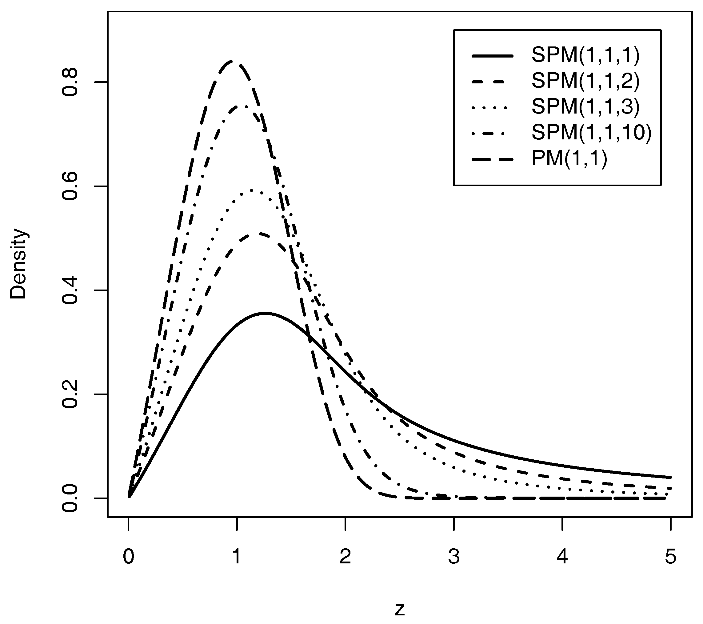
We perform a brief comparison illustrating that the tails of the SPM distribution are heavier than those of the PM distribution.

Table 1. Tails comparison for different SPM and PM distributions.

Distribution	$\mathit{P}(\mathit{Z}>3)$	$\mathit{P}(\mathit{Z}>4)$	$\mathit{P}(\mathit{Z}>5)$
PM(1,1)	$2.09·{10}^{-6}$	$1.98·{10}^{-20}$	$7.35·{10}^{-60}$
SPM(1,1,10)	0.00360	0.00015	$1.31·{10}^{-5}$
SPM(1,1,3)	0.05910	0.01870	0.00765
SPM(1,1,2)	0.08834	0.03727	0.01908
SPM(1,1,1)	0.11111	0.06250	0.04000

shows $P(Z>z)$ for different values of z in the distributions mentioned. We noted that the SPM distribution has much heavier tails than the PM distribution. Figure 1 depicts examples of the SPM distribution for different values the parameters.

2.3. Probabilistic Properties

In this subsection, we study basic properties of the SPM distribution.

Proposition 2.

Let $Z\sim SPM(\beta ,\gamma ,q)$. Then, the cdf of Z is given by

$$F_Z(z;\beta ,\gamma ,q)=eq{\beta }^q\Gamma \left(\frac{q}{\gamma }+1\right)\left\{E_{I_{-1}}(z)-E_{I_0}(z)\right\},z>0,$$

where ${\displaystyle E_{I_r}(z)={\int }_0^z\frac{1}{t^{q+1}}{E}_r^{q/\gamma }(1;v_t)dt}$ of $r=-1,0$ and $v_t=exp\left\{{\left(\frac{t}{\beta }\right)}^{\gamma }\right\}$.

Proof. 

Using cfd definition. □

Proposition 3.

Let $Z\sim SPM(\beta ,\gamma ,q)$. If $q\to \infty$, then Z converges in law to a random variable $X\sim PM(\beta ,\gamma )$.

Proof. 

Let $Z\sim SPM(\beta ,\gamma ,q)$. Then, Z can be represented as $Z=\frac{X}{U^{1/q}}$. First, we study the probability convergence of $U^{1/q}$.

Since $U\sim U(0,1)$ and if $W=U^{1/q}$, then $W\sim Beta(q,1)$. Hence, we have $E\left[{(W-1)}^2\right]=\frac{2}{(q+1)(q+2)}$ that converges to 0 as $q\to \infty$, which implies that $W\stackrel{\mathcal{P}}{\to }1$. Thus, applying Slutsky lemma finishes the proof of the proposition. □

Proposition 4.

If $Z|T=t\sim PM(\beta t^{-1/q},\gamma )$ and $T\sim U(0,1)$, then $Z\sim SPM(\beta ,\gamma ,q)$.

Proof. 

By noting that the marginal pdf of Z is given by

$$\begin{array}{ccc}\hfill f_Z(z;\beta ,\gamma ,q)& =& {\int }_0^1{f}_{Z|T}(z|t)f_T(t)dt\hfill \\ & =& {\int }_0^1\frac{\gamma }{{(\beta t^{-1/q})}^{\gamma }}{z}^{\gamma -1}\left(e^{{\left(\frac{z}{\beta t^{-1/q}}\right)}^{\gamma }}-1\right)exp\left({\left(\frac{z}{\beta t^{-1/q}}\right)}^{\gamma }-e^{{\left(\frac{z}{\beta t^{-1/q}}\right)}^{\gamma }}+1\right)dt.\hfill \end{array}$$

Then, marking the transformation variable ${\displaystyle v={\left(\frac{z}{\beta t^{-1/q}}\right)}^{\gamma }}$ where ${\displaystyle dv=\frac{\gamma v}{q}{t}^{-1}dt}$ and ${\displaystyle t^{-1}=\frac{z^q}{{\beta }^q{v}^{q/v}}}$, by some algebraic adjustments, we get (4). □

2.4. Moments

Proposition 5.

Let $Z\sim SPM(\beta ,\gamma ,q)$. Then, for $r=1,2,\dots$ and $q>r$, it follows that the r-th moment of Z can be written as

$${\mu }_r=E(Z^r)=\frac{e{\beta }^{r}q}{q-r}{M}_r(\gamma ),$$

where $M_r=M_r(\gamma )=\Gamma \left(\frac{r}{\gamma }+1\right)E_0^{\frac{r}{\gamma }-1}(1)$.

Proof. 

Using the stochastic representation for the distribution given in (3), we have that

$${\mu }_r=E\left(Z^r\right)=E\left({\left(\frac{X}{U^{1/q}}\right)}^r\right)=E\left(X^r{U}^{-r/q}\right)=E\left(X^r\right)E\left(U^{-r/q}\right),$$

where $E\left(U^{-r/q}\right)=\frac{q}{q-r},q>r$ and $E\left(X^r\right)=e{\beta }^r\Gamma \left(\frac{r}{\gamma }+1\right)E_0^{\frac{r}{\gamma }-1}(1)$ are the moments of the $PM(\beta ,\gamma )$ distribution. □

Corollary 1.

If $Z\sim SPM(\beta ,\gamma ,q)$, then it follows that

1. 

${\mu }_1=E(Z)=\frac{e\beta q}{q-1}{M}_1(\gamma )q>1;$

2. 

${\mu }_2=E(Z^2)=\frac{e{\beta }^{2}q}{q-2}{M}_2(\gamma )q>2;$

3. 

${\mu }_3=E(Z^3)=\frac{e{\beta }^{3}q}{q-3}{M}_3(\gamma )q>3;$

4. 

${\mu }_4=E(Z^4)=\frac{e{\beta }^{4}q}{q-4}{M}_4(\gamma )q>4.$

Corollary 2.

Let $Z\sim SPM(\beta ,\gamma ,q)$, then the asymmetry coefficient, ($\sqrt{{\beta }_1}$) and the kurtosis coefficient (${\beta }_2$) for $q>3$ and $q>4$ are, respectively,

$$\begin{array}{ccc}\hfill \sqrt{{\beta }_1}& =& \frac{\sqrt{q-2}\left\{{(q-1)}^3(q-2)M_3-3eq{M}_1{M}_2{(q-1)}^2(q-3)+2e^2{q}^2{M}_1^3(q-2)(q-3)\right\}}{\sqrt{eq}(q-3){\left\{(q-1)M_2-eq(q-2)M_1^2\right\}}^{3/2}},\hfill \\ \hfill {\beta }_2& =& \frac{{(q-1)}^3{(q-2)}^{2}A+3(q-2)(q-3)(q-4)e^2{q}^{2}B}{eq(q-3)(q-4){\left\{(q-1)M_2-eq(q-2)M_1^2\right\}}^2},\hfill \end{array}$$

where $A=(q-1)(q-3)M_4-4eq(q-4)M_1{M}_3$ and $B=2{(q-1)}^2{M}_1^2{M}_2-eq(q-2)M_1^4.$

Remark 1.

The asymmetry and kurtosis coefficients were obtained using:

$$\sqrt{{\beta }_1}=\frac{{\mu }_3-3{\mu }_1{\mu }_2+2{\mu }_1^3}{{({\mu }_2-{\mu }_1^2)}^{\frac{3}{2}}}and{\beta }_2=\frac{{\mu }_4-4{\mu }_1{\mu }_3+6{\mu }_2{\mu }_1^2-3{\mu }_1^4}{{({\mu }_2-{\mu }_1^2)}^2}.$$

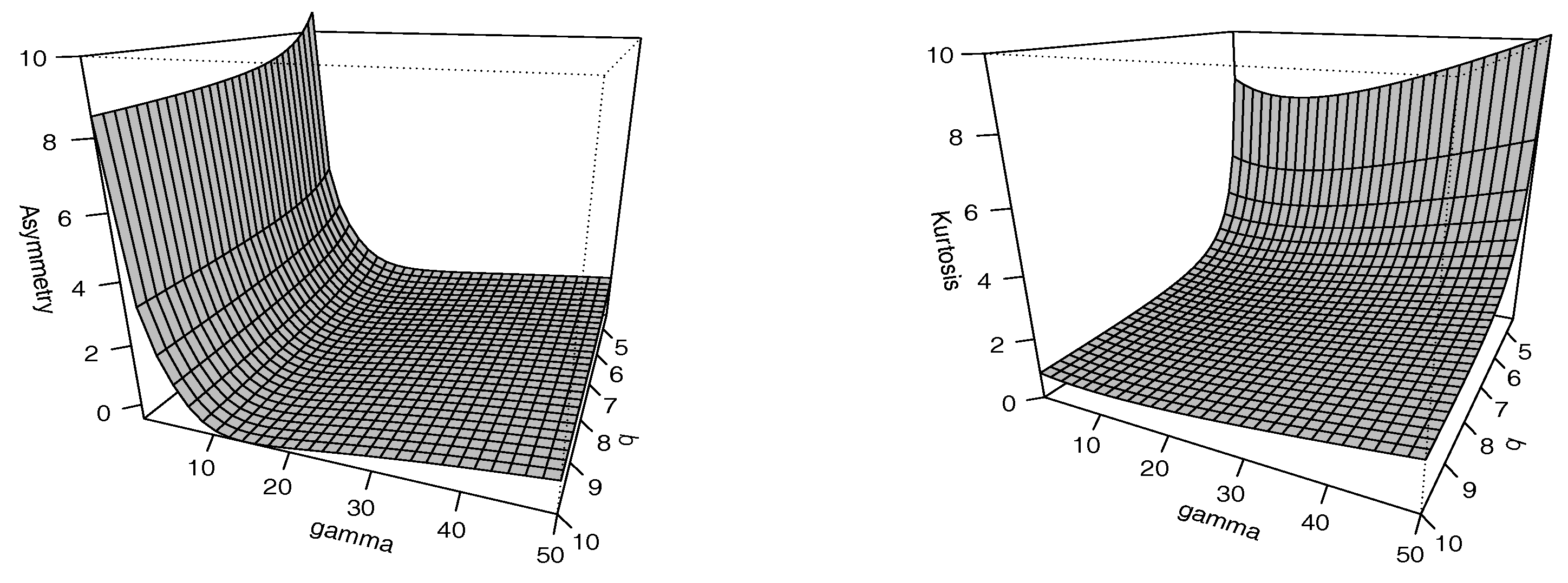
Figure 2 shows the skewness and kurtosis coefficients of the SPM model for different values of q and $\gamma$; we can see that for small values of q the kurtosis coefficient increases in the SPM model. The ranges of both coefficients are larger than those of the PM model (see Jodrá et al. [18]). Thus, the SPM model is more flexible than the PM model for modeling data with larger coefficients of asymmetry and kurtosis.

3. Inference

In this section, we address the problem of estimating parameters of the SPM distribution. In Section 3.1, we apply moment estimation and, in Section 3.2, we describe the ML method. Finally, in Section 3.3, we present some simulation results. For the following subsections, we consider $Z_1,\cdots ,Z_n$ be a random sample of size n from the $SPM(\beta ,\gamma ,q)$ distribution with parameters $\beta$, $\gamma$, q and $z_1$, $z_2$, ..., $z_n$ the observed values of the sample.

3.1. Moment Method Estimators

Rewriting the first moment with $\beta$ isolated and replacing E(Z) by the sample mean $\overline{Z}$, we have the equation

$$\beta =\frac{\overline{Z}(q-1)}{eq{M}_1(\gamma )}.$$

(5)

Therefore, using (5) and replacing the second and third population moments by the corresponding second and third sampling moments, we obtain the following equations:

$$\overline{Z^2}=\frac{{\overline{Z}}^2{(q-1)}^2{M}_2(\gamma )}{eq(q-2)M_1^2(\gamma )};$$

(6)

$$\overline{Z^3}=\frac{{\overline{Z}}^3{(q-1)}^3{M}_3(\gamma )}{e^2{q}^2(q-3)M_1^3(\gamma )}.$$

(7)

The system of equations generated by (6) and (7) needs to be solved numerically using $\mathtt{R}-\mathtt{project}$, leading to the estimators ${\widehat{\gamma }}_M$ and ${\widehat{q}}_M$. The estimator ${\widehat{\beta }}_M$ is obtained from Equation (5) , replacing q by ${\widehat{q}}_M$ and computing $M_1(\gamma )$ by using estimator $M_1({\widehat{\gamma }}_M)$.

3.2. Ml Estimation

The log-likelihood (ℓ) function can be written as follows:

$$\ell (\Theta )=c(\beta ,q)+nlog\left\{\Gamma \left(\frac{q}{\gamma }+1\right)\right\}-(1+q)\sum _{i=1}^{n}log(z_i)+\sum _{i=1}^{n}log\left\{E_{-1}^{\frac{q}{\gamma }}\left(1;v_i\right)-E_0^{\frac{q}{\gamma }}\left(1;v_i\right)\right\},$$

where $\Theta =(\beta ,\gamma ,q)$, $c(\beta ,q)=n+nlog(q)+nqlog(\beta )$ and $v_i=exp\left\{{\left(\frac{z_i}{\beta }\right)}^{\gamma }\right\}$, $i=1,\dots ,n$. Then, the ML equations are given by

$$\begin{array}{ccc}\hfill \frac{{\beta }^{-q}}{e\Gamma \left(\frac{q}{\gamma }+1\right)}\sum _{i=1}^n\frac{z_i^{q+1}{f}_X(z_i;\beta ,\gamma )}{E_{-1}^{\frac{q}{\gamma }}\left(1;v_i\right)-E_0^{\frac{q}{\gamma }}\left(1;v_i\right)}& =& nq\hfill \end{array}$$

(8)

$$\begin{array}{ccc}\hfill \frac{\beta {\gamma }^2}{qe}\sum _{i=1}^n\frac{{\left(\frac{z_i}{\beta }\right)}^{q+1}log\left(\frac{z_i}{\beta }\right)f_X(z_i;\beta ,\gamma )}{E_{-1}^{\frac{q}{\gamma }}\left(1;v_i\right)-E_0^{\frac{q}{\gamma }}\left(1;v_i\right)}& =& \sum _{i=1}^n\frac{\kappa (z_i)}{E_{-1}^{\frac{q}{\gamma }}\left(1;v_i\right)-E_0^{\frac{q}{\gamma }}\left(1;v_i\right)}\hfill \end{array}$$

(9)

$$\begin{array}{ccc}\hfill \gamma \Gamma \left(\frac{q}{\gamma }+1\right)\left\{\sum _{i=1}^{n}log(z_i)-\frac{n}{q}-nlog(\beta )\right\}& =& \sum _{i=1}^n\frac{\kappa (z_i)}{E_{-1}^{\frac{q}{\gamma }}\left(1;v_i\right)-E_0^{\frac{q}{\gamma }}\left(1;v_i\right)}\hfill \end{array}$$

(10)

where $f_X(·)$ is given in (1) and $\kappa (z_i)={\int }_1^{v_i}log(log(u)){\left(log(u)\right)}^{q/\gamma }(u-1)e^{-u}du$, with $i=1,\dots ,n$.

Solutions for Equations (8)–(10) can be obtained using numerical procedures such as the Newton–Raphson procedure.

3.3. Simulation Study

By using the stochastic representation given in (3), it is possible to generate random numbers of a random variable $SPM(\beta ,\gamma ,q)$ distribution with the following algorithm:

• Simulate $U\sim Uniform(0,1).$
• Compute $V=\beta {\left(log\left\{-W_{-1}\left(\frac{U-1}{e}\right)\right\}\right)}^{1/\gamma },$ where W is the Lambert W function.
• Compute $Z=\frac{V}{U^{1/q}}.$

It then follows that $Z\sim SPM(\beta ,\gamma ,q)$.

Table 2. Simulation of 1000 iterations for the $SPM(\beta ,\gamma ,q)$ model.

n	$\mathit{\beta }$	$\mathit{\gamma }$	q	$\widehat{\mathit{\beta }}$	$\mathit{SD}(\widehat{\mathit{\beta }})$	$\mathit{C}(\widehat{\mathit{\beta }})$	$\widehat{\mathit{\gamma }}$	$\mathit{SD}(\widehat{\mathit{\gamma }})$	$\mathit{C}(\widehat{\mathit{\gamma }})$	$\widehat{\mathit{q}}$	$\mathit{SD}(\widehat{\mathit{q}})$	$\mathit{C}(\widehat{\mathit{q}})$
50	1	1	2	1.0391	0.1372	91.6	1.0535	0.2106	91.8	2.3550	0.8728	95.4
100	1	1	2	1.0260	0.0934	93.0	1.0234	0.1399	91.8	2.2321	0.4495	95.3
150	1	1	2	1.0163	0.0752	92.5	1.0089	0.1112	93.5	2.1538	0.3294	95.0
200	1	1	2	1.0182	0.0651	92.0	0.9981	0.0943	91.1	2.1515	0.2798	92.9
50	1	1	3	1.0078	0.1227	92.9	1.0701	0.1963	93.5	3.3892	1.5270	93.1
100	1	1	3	1.0125	0.0880	93.9	1.0214	0.1290	94.0	3.3267	0.9484	95.0
150	1	1	3	1.0019	0.0694	93.3	1.0107	0.1028	94.3	3.1859	0.6382	94.6
200	1	1	3	1.0076	0.0609	94.6	1.0039	0.0880	94.8	3.1639	0.5385	95.4
50	1	1	4	0.9766	0.1179	93.4	1.0465	0.1862	95.0	4.1195	2.1138	89.4
100	1	1	4	1.0065	0.0852	94.2	1.0174	0.1216	95.2	4.4275	1.5731	95.3
150	1	1	4	1.0115	0.0699	94.7	1.0015	0.0960	95.5	4.3927	1.2308	94.9
200	1	1	4	1.0109	0.0597	95.0	0.9999	0.0823	93.5	4.3101	0.9668	95.1
50	3	1	2	2.9590	0.4196	92.0	1.0179	0.2117	94.0	2.3601	0.7448	98.0
100	3	1	2	3.1021	0.3145	98.0	1.0034	0.1495	96.0	2.4675	0.5667	100.0
150	3	1	2	3.1885	0.2512	92.0	1.0075	0.1156	98.0	2.6076	0.4875	100.0
200	3	1	2	3.1785	0.2199	94.0	0.9806	0.0982	94.0	2.6012	0.4217	90.0
50	2	1	2	2.0166	0.2702	94.0	1.0699	0.2161	86.0	2.3286	0.7356	94.0
100	2	1	2	2.0362	0.1823	92.0	1.0260	0.1374	92.0	2.2804	0.4400	98.0
150	2	1	2	2.0972	0.1616	92.0	0.9978	0.1112	90.0	2.4041	0.4160	98.0
200	2	1	2	2.1220	0.1372	86.0	0.9856	0.0903	88.0	2.4925	0.3741	96.0

shows the results of simulations studies illustrating the behavior of the ML estimates for 1000 generated samples of sizes 50, 100, 150, and 200 from a population with $SPM(\beta ,\gamma ,q)$ distribution. For each sample generated, ML estimates were computed numerically using a Newton–Raphson procedure. Means, standard deviations (SD), and empirical coverage (C) based on a confidence interval of 95%. It is observed that the bias becomes smaller as the sample size n increases, as one would expect.

4. Applications

In this section, we consider two real data sets to illustrate that the SPM distribution may be more suitable than the PM distribution for modeling data with excess kurtosis.

4.1. Application I (Rubidium Concentration)

We consider Rubidium concentration data from 86 soil samples obtained by the Mining Department of Universidad de Atacama, Chile. Statistical measurements and the ML estimates of the SPM distribution were obtained and compared with the PM distribution with its standard errors.

Table 3. Summary statistics for Rubidium concentration.

n	$\overline{\mathit{z}}$	${\mathit{s}}^2$	${\mathit{b}}_1$	${\mathit{b}}_2$
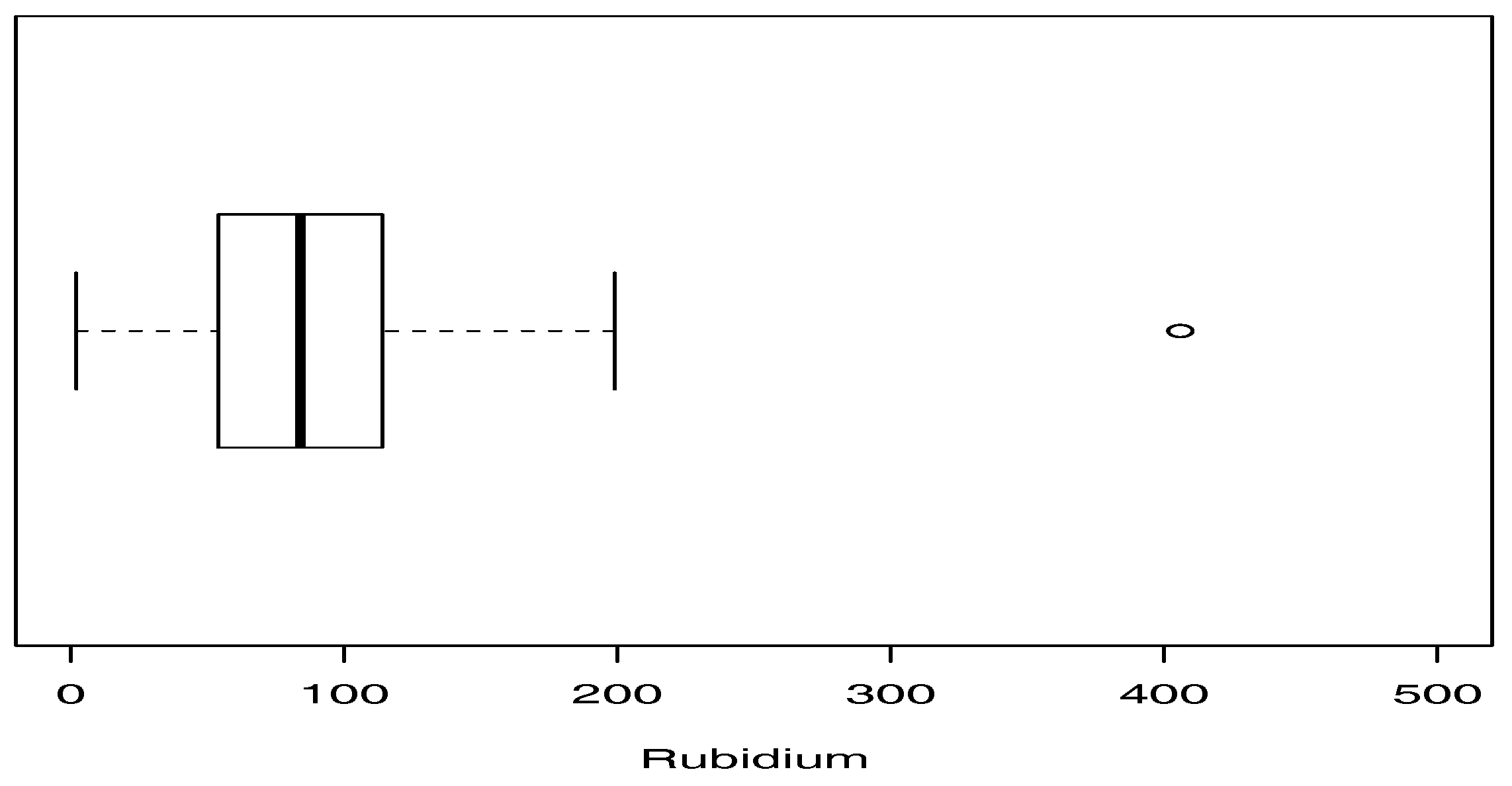
86	88.5698	56.4683	2.1948	13.4317

shows some descriptive statistics for the data set, where $b_1$ and $b_2$ denote the skewness and kurtosis coefficients, respectively, of the sample. In this respect, we highlight the high kurtosis of this data. Figure 3 presents a boxplot for the data, where an atypical observation is noted. From the results in Section 3.1, the moment estimates for the parameters of the SPM model are ${\widehat{\beta }}_M=66.704$, ${\widehat{\gamma }}_M=0.825$ and ${\widehat{q}}_M=4.397$. These estimates are used as the initial values needed to implement estimation by the ML method using the numerical method.

In

Table 4. Parameter estimates, standard error (SE), and values for PM and SPM models for Rubidium concentration.

Parameter Estimates	PM (SE)	SPM (SE)
$\beta$	81.6487 (6.6748)	67.6313 (6.0901)
$\gamma$	0.6311 (0.0468)	0.6398 (0.0890)
q		4.7829 (1.9498)
AIC	922.1212	910.826
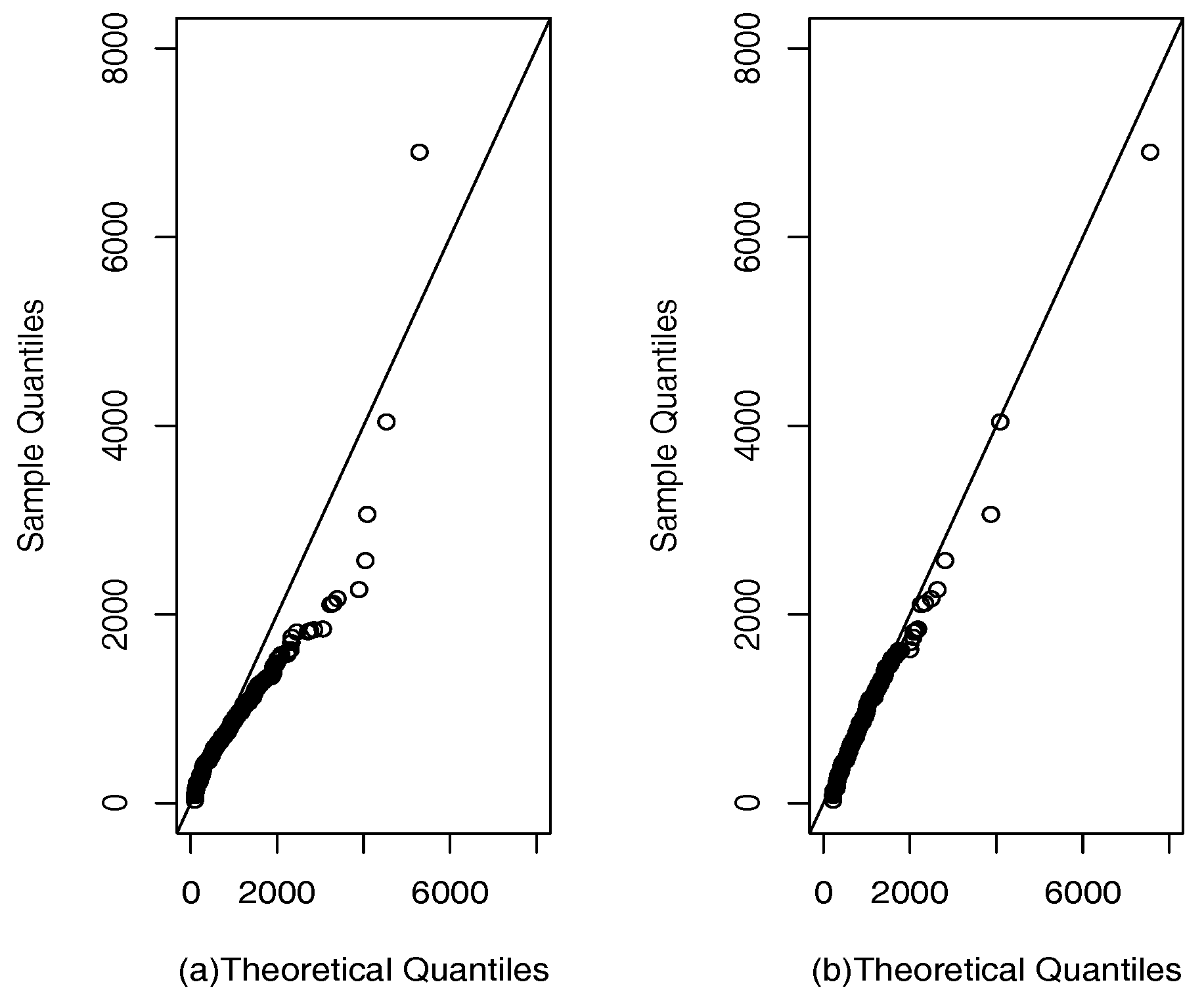
BIC	927.030	918.188

, we compare the SPM and PM models. We calculated the Akaike information criterion AIC (see Akaike [20]) and the Bayesian information criterion BIC (see Schwartz [21]). It can be seen that AIC and BIC show a better fit of the SPM model, and the qqplots in Figure 4 show that the SPM model fits better than the PM model.

4.2. Application II (Dietary Retinol Consumed)

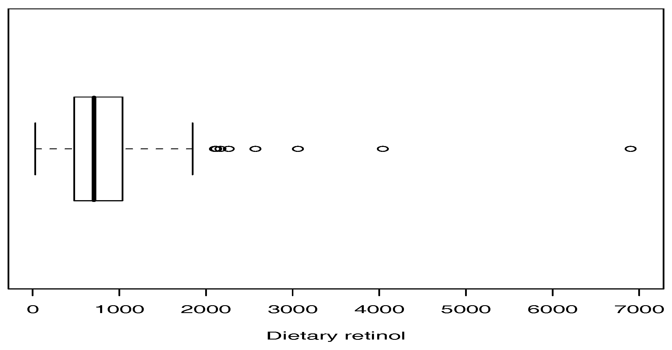
The real data were obtained from a cross-sectional study to investigate the relation between personal characteristics and dietetic factors dietéticos, and plasma concentrations of retinol, beta-carotene, and other carotenoids in 315 patients. The data set is available online at “http://lib.stat.cmu.edu/datasets/Plasma_Retinol” and contains 14 variables. The data consist of dietary retinol consumed by 315 patients (mcg per day).

Table 5. Summary statistics for the dietary retinol concentration.

n	$\overline{\mathit{z}}$	${\mathit{s}}^2$	${\mathit{b}}_1$	${\mathit{b}}_2$
315	832.7143	347261.600	4.453	40.447

shows some descriptive statistics for the data set, in which we highlight the very high kurtosis of the data. Figure 5 presents a boxplot for the data, which shows that there are several outliers. From the results in Section 3.1, the moment estimates for the parameters of the SPM model are ${\widehat{\beta }}_M=586.181$, ${\widehat{\gamma }}_M=0.785$ and ${\widehat{q}}_M=3.682$. These estimates are used as initial values for calculating the ML estimates.

Table 6. Parameter estimates, (SE) indicates standard error estimates, and log-likelihood values for PM and SPM models for the dietary retinol concentration.

Parameter Estimates	PM (SE)	SPM (SE)
$\beta$	755.999 (35.916)	566.988 (29.268)
$\gamma$	0.566 (0.019)	1.024 (0.078)
q	−	3.110 (0.437)
AIC	4810.924	4699.180
BIC	4818.429	4710.438

shows the ML estimates for the parameters of the SPM and PM models. For each model, we report the corresponding AIC and BIC values. It can be seen that AIC and BIC show better fit in the SPM model, and, when there are more atypical observations, the fit of the SPM model is much better. Finally, the qqplots in Figure 6 show that the SPM model fits better than the PM model.

5. Discussion

We have presented a new extension of the PM model, called the slash Power Muth model. It is defined on the basis of the principle used to produce the slash distribution, but using the PM model instead of the normal model. Thus, the PM model is a special case of the SPM model.

We studied properties of the SPM distribution including stochastic representation, moments, asymmetry, and kurtosis. Parameters are estimated using the moment method and ML method. The results of a simulation study show good parameter recovery. Some other characteristics of the new model are:

• The density of the SPM model has a closed-form and is expressed in terms of the incomplete generalized integro-exponential function.
• The SPM model presents more flexible coefficients of asymmetry and kurtosis than those of the PM model. Furthermore, as shown in Table 1, the tails become heavier when the parameter q is smaller.
• We discuss two stochastic representations for the SPM model: one is based on the quotient between two independent random variables, a PM in the numerator, and a power of a U in the denominator; the other is obtained as a mixture of the scale of a PM model and a U model.
• The moments and coefficients of asymmetry and kurtosis have closed-form expressions and are expressed in terms of the generalized integro-exponential function.
• In the applications, two criteria (AIC and BIC) were used to compare the models. In both data sets, the coefficient of kurtosis is high, indicating the presence of atypical observations. The criteria indicate that the SPM model provides the best fit to the data.
• The SPM distribution is a good alternative for modeling continuous positive data sets with atypical observations. These situations are common in all areas of knowledge, for example environmental science, economic, geo-chemistry, survival, reliability, etc. In the future, we will use this distribution in problems of regression, reliability, survival analysis, and Bayesian inference.

References

- Johnson, N.L.; Kotz, S.; Balakrishnan, N. Continuous Univariate Distributions, 2nd ed.; Wiley-Interscience: New York, NY, USA, 1994; Volume 1. [Google Scholar]
- Rogers, W.H.; Tukey, J.W. Understanding some long-tailed symmetrical distributions. Statist. Neerl. 1972, 26, 211–226. [Google Scholar] [CrossRef]
- Mosteller, F.; Tukey, J.W. Data Analysis and Regression; Addison-Wesley: Boston, MA, USA, 1977. [Google Scholar]
- Kafadar, K. A biweight approach to the one-sample problem. J. Am. Stat. Assoc. 1982, 77, 416–424. [Google Scholar] [CrossRef]
- Gómez, H.W.; Quintana, F.A.; Torres, F.J. New Family of Slash-Distributions with Elliptical Contours. Stat. Probabil. Lett. 2007, 77, 717–725. [Google Scholar] [CrossRef]
- Gómez, H.W.; Venegas, O. Erratum to: A New Family of Slash-Distributions with Elliptical Contours. Stat. Probab. Lett. 2008, 78, 2273–2274. [Google Scholar] [CrossRef]
- Gómez, H.W.; Olivares-Pacheco, J.F.; Bolfarine, H. An extension of the generalized Birnbaum–Saunders distribution. Stat. Probab. Lett. 2009, 79, 331–338. [Google Scholar] [CrossRef]
- Olmos, N.M.; Varela, H.; Gómez, H.W.; Bolfarine, H. An extension of the half-normal distribution. Stat. Pap. 2012, 53, 875–886. [Google Scholar] [CrossRef]
- Olmos, N.M.; Varela, H.; Bolfarine, H.; Gómez, H.W. An extension of the generalized half-normal distribution. Stat. Pap. 2014, 55, 967–981. [Google Scholar] [CrossRef]
- Reyes, J.; Barranco-Chamorro, I.; Gallardo, D.I.; Gómez, H.W. Generalized modified slash Birnbaum–Saunders distribution. Symmetry 2018, 10, 724. [Google Scholar] [CrossRef] [Green Version]
- Gómez, Y.M.; Bolfarine, H.; Gómez, H.W. Gumbel distribution with heavy tails and applications to environmental data. Math. Comput. Simul. 2019, 157, 115–129. [Google Scholar] [CrossRef]
- Segovia, F.A.; Gómez, Y.M.; Venegas, O.; Gómez, H.W. A power Maxwell distribution with heavy tails and applications. Mathematics 2020, 8, 1116. [Google Scholar] [CrossRef]
- Muth, J.E. Reliability models with positive memory derived from the mean residual life function. In The Theory and Applications of Reliability; Tsokos, C.P., Shimi, I., Eds.; Academic Press: New York, NY, USA, 1977; Volume II, pp. 401–435. [Google Scholar]
- Jodrá, P.; Jiménez-Gamero, M.D.; Alba-Fernández, M.V. On the Muth Distribution. Math. Model. Anal. 2015, 20, 291–310. [Google Scholar] [CrossRef]
- Milgram, M.S. The generalized integro-exponential function. Math. Comput. 1985, 44, 443–458. [Google Scholar] [CrossRef]
- Chiccoli, C.; Lorenzutta, S.; Maino, G. A numerical method for generalized exponential integrals. Comp. Math. Applic. 1987, 14, 261–268. [Google Scholar] [CrossRef] [Green Version]
- Chiccoli, C.; Lorenzutta, S.; Maino, G. Recent results for generalized exponential integrals. Comp. Math. Applic. 1990, 19, 21–29. [Google Scholar] [CrossRef] [Green Version]
- Jodrá, P.; Gómez, H.W.; Jiménez-Gamero, M.D.; Alba-Fernández, M.V. The power Muth distribution. Math. Model. Anal. 2017, 22, 186–201. [Google Scholar] [CrossRef]
- Corless, R.M.; Gonnet, G.H.; Hare, D.E.G.; Jeffrey, D.J.; Knuth, D.E. On the Lambert W function. Adv. Comput. Math. 1996, 5, 329–359. [Google Scholar] [CrossRef]
- Akaike, H. A new look at the statistical model identification. IEEE Trans. Autom. Control 1974, 19, 716–723. [Google Scholar] [CrossRef]
- Schwarz, G. Estimating the dimension of a model. Ann. Stat. 1978, 6, 461–464. [Google Scholar] [CrossRef]
Figure 1.
Plot of the SPM distribution.
Figure 2.
Asymmetry coefficient (left) and kurtosis coefficient (right) for SPM distribution.
Figure 3.
Boxplot for rubidium dataset.
Figure 4.
qqplots for rubidium dataset: (a) PM model; (b) SPM model.
Figure 5.
Boxplot for retinol dataset.
Figure 6.
qqplots for retinol dataset: (a) PM model; (b) SPM model.