
An Exhaustive Power Comparison of Normality Tests


1
Department of Applied Mathematics, Kaunas University of Technology, 51368 Kaunas, Lithuania
2
Department of Computer Sciences, Kaunas University of Technology, 51368 Kaunas, Lithuania
3
Department of Mathematical modelling, Kaunas University of Technology, 51368 Kaunas, Lithuania
*
Author to whom correspondence should be addressed.
Mathematics 2021, 9(7), 788; https://doi.org/10.3390/math9070788
Submission received: 12 February 2021
/
Revised: 17 March 2021
/
Accepted: 31 March 2021
/
Published: 6 April 2021
(This article belongs to the Special Issue Probability, Statistics and Their Applications 2021)
Abstract
:A goodness-of-fit test is a frequently used modern statistics tool. However, it is still unclear what the most reliable approach is to check assumptions about data set normality. A particular data set (especially with a small number of observations) only partly describes the process, which leaves many options for the interpretation of its true distribution. As a consequence, many goodness-of-fit statistical tests have been developed, the power of which depends on particular circumstances (i.e., sample size, outlets, etc.). With the aim of developing a more universal goodness-of-fit test, we propose an approach based on an N-metric with our chosen kernel function. To compare the power of 40 normality tests, the goodness-of-fit hypothesis was tested for 15 data distributions with 6 different sample sizes. Based on exhaustive comparative research results, we recommend the use of our test for samples of size .
1. Introduction
A priori information about data distribution is not always known. In those cases, hypothesis testing can help to find a reasonable assumption about the distribution of data. Based on assumed data distribution, one can choose appropriate methods for further research. The information about data distribution can be useful in a number of ways, for example:
- it can provide insights about the observed process;
- parameters of model can be inferred from the characteristics of data distributions; and
- it can help in choosing more specific and computationally efficient methods.
Statistical methods often require data to be normally distributed. If the assumption of normality is not satisfied, the results of these methods will be inappropriate. Therefore, the presumption of normality is strictly required before starting the statistical analysis. Many tests have been developed to check this assumption. However, tests are defined in various ways and thus react to abnormalities, present in a data set, differently. Therefore, the choice of goodness-of-fit test remains an important problem.
For these reasons, this study examines the issue of testing the goodness-of-fit hypotheses. The goodness-of-fit null and alternative hypotheses are defined as:
A total of 40 tests were applied to analyze the problem of testing the goodness-of-fit hypothesis. The tests used in this study were developed between 1900 and 2016. In the early 19th century, Karl Pearson published an article defining the chi-square test [1]. This test is considered as the basis of modern statistics. Pearson was the first to examine the goodness-of-fit assumption that the observations can be distributed according to the normal distribution, and concluded that, in the limit as becomes large, follows the chi-square distribution with degrees of freedom. The statistics for this test are defined in Section 2.1. Another popular test for testing the goodness-of-fit hypothesis is the Kolmogorov and Smirnov test [2]. This test statistic quantifies a distance between the empirical distribution function of the sample and the cumulative distribution function of the reference distribution [3]. The Anderson and Darling test is also often used in practice [4]. This test assesses whether a sample comes from a specified distribution [3]. The end of 19th century and the beginning of 20th century was a successful period for the development of goodness-of-fit hypothesis test criteria and their comparison studies [5,6,7,8,9,10,11,12,13,14,15,16,17,18,19].
In 2010, Xavier Romão et al. conducted a comprehensive study comparing the power of the goodness-of-fit hypothesis tests [20]. In the study, 33 normality tests were applied to samples of different sizes, taking into account the significance level and many symmetric, asymmetric, and modified normal distributions. The researchers found that the most powerful of the selected normality tests for the symmetric group of distributions were Coin , Chen–Shapiro, Bonett–Seier, and Gel–Miao–Gastwirth tests; for the asymmetric group of distributions, Zhang–Wu and , and Chen–Shapiro; while the Chen–Shapiro, Barrio–Cuesta-Albertos–Matrán–Rodríguez-Rodríguez, and Shapiro–Wilk tests were the most powerful for the group of modified normal distributions.
In 2015, Adefisoye et al. compared 18 normality tests for different sample sizes for symmetric and asymmetric distribution groups [3]. The results of the study showed that the Kurtosis test was the most powerful for a group of symmetric data distributions and the Shapiro–Wilk test was the most powerful for a group of asymmetric data distributions.
The main objective of this study is to perform a comparative analysis of the power of the most commonly used tests for testing the goodness-of-fit hypothesis. The procedure described in Section 3 was used to calculate the power of the tests.
Scientific novelty—the comparative analysis of test power was carried out using different methods for goodness-of-fit in the case of many different types of challenges to curve tests. The goodness-of-fit tests have been selected as representatives of popular techniques, which have been analyzed by other researchers experimentally. We have proposed a new kernel function and its usage in an N-metric-based test. The uniqueness of the kernel function is that its shape is chosen in such a way that the shift arising in the formation of the test is eliminated by using sample values.
The rest of the paper is organized as follows. Section 2 provides descriptions of the 40 goodness-of-fit hypothesis tests and the procedure for calculating the power of the tests. The samples generated from 15 distributions are given in Section 4. Section 5 presents and discusses the results of a simulation modeling study. Finally, Section 6 concludes the results.
2. Statistical Methods
In this section, the most popular tests for normality are overviewed.
2.1. Chi-Square Test (CHI2)
In 1900, Karl Pearson introduced the chi-square test [1]. The statistic of the test is defined as:
where is the observed frequency and is the expected frequency.
2.2. Kolmogorov–Smirnov (KS)
In 1933, Kolmogorov and Smirnov proposed the KS test [2]. The statistic of the test is defined as:
where is the cumulative probability of standard normal distribution and is the difference between observed and expected values.
2.3. Anderson–Darling (AD)
In 1952, Anderson and Darling developed a variety of the Kolmogorov and Smirnov tests [4]. This test is more powerful than the Kolmogorov and Smirnov test. The statistic of the test is defined as:
where the value of the distribution function at point and empirical sample size.
2.4. Cramer–Von Mises (CVM)
In 1962, Cramer proposed the Cramer–von Mises test. This test is an alternative to the Kolmogorov and Smirnov test [21]. The statistic of the test is defined as:
where is the cumulative distribution function of the specified distribution and are the sample mean and sample standard deviation.
2.5. Shapiro–Wilk (SW)
In 1965, Shapiro and Wilk formed the original test [22]. The statistic of the test is defined as:
where is the order statistic, is the sample mean, and constants obtained:
where are the expected values of the order statistics of independent and identically distributed random variables sampled from the standard normal distribution and is the covariance matrix of those order statistics.
2.6. Lilliefors (LF)
In 1967, Lilliefors modified the Kolmogorov and Smirnov test [23]. The statistic of the test is defined as:
where the standard normal distribution function and the empirical distribution function of the values.
2.7. D’Agostino (DA)
In 1971, D’Agostino introduced the test for testing the goodness-of-fit hypothesis, which is an extension of the Shapiro–Wilk test [8]. The test proposed by D’Agostino does not need to define a weight vector. The statistic of the test is defined as:
where is the second central moment that is defined as:
2.8. Shapiro–Francia (SF)
In 1972, Shapiro and Francia simplified the Shapiro and Wilk test and developed the Shapiro and Francia test, which is computationally more efficient [24]. The statistic of the test is defined as:
where the expected values of the standard normal order statistics.
2.9. D’Agostino–Pearson (DAP)
In 1973–1974, D’Agostino and Pearson proposed the D’Agostino and Pearson test [25]. The statistic of the test is defined as:
where is the size of sample and is the sample variance of order statistics.
2.10. Filliben (Filli)
In 1975, Filliben defined the probabilistic correlation coefficient as a test for the goodness-of-fit hypothesis [26]. This test statistic is defined as:
where the variance,, when the estimated median values of the order statistics, each is obtained by:
2.11. Martinez–Iglewicz (MI)
In 1981, Martinez and Iglewicz proposed a normality test based on the ratio of two estimators of variance, where one of the estimators is the robust biweight scale estimator [27]:
where is the sample median, , with being the median of .
This test statistic is then given by:
2.12. Epps–Pulley (EP)
In 1983, Epps and Pulley proposed a test statistic based on the following weighted integral [28]:
where is the empirical characteristic function and is an adequate function chosen according to several considerations. By setting and selecting:
the following statistic is obtained:
where the second central moment.
2.13. Jarque–Bera (JB)
In 1987, Jarque and Bera proposed a test [29] with statistic defined as:
where and are the sample skewness and kurtosis.
2.14. Hosking (
In 1990, Hosking and Wallis proposed the first Hosking test [5]. This test statistic is defined as:
where and are the mean and standard deviation of number of simulation data values of is calculated as:
where coefficient of variation of the L-moment ratio, coefficient of skewness of the L- moment, and is the coefficient of kurtosis of the L- moment.
2.15. Cabaña–Cabaña (CC1-CC2)
In 1994, Cabaña and Cabaña proposed the CC1 and CC2 tests [6]. The CC1 () and CC2 (), respectively, are defined as:
whereand approximate transformed estimated empirical processes sensitive to changes in skewness and kurtosis and are defined as:
where a dimensionality parameter, the probability density function of the standard normal distribution, the th order normalized Hermite polynomial, and theth order normalized mean of the Hermite polynomial defined as:
2.16. The Chen–Shapiro Test (ChenS)
In 1995, Chen and Shapiro introduced an alternative test statistic based on normalized spacings and defined as [9]:
where the th quantile of a standard normal distribution.
2.17. Modified Shapiro-Wilk (SWRG)
In 1997, Rahman and Govindarajulu proposed a modification to the Shapiro–Wilk test [8]. This test statistic is simpler to compute and relies on a new definition of the weights using the approximations to and . Each element of the weight vector is given as:
where it is assumed that . Therefore, the modified test statistic assigns larger weights to the extreme order statistics than the original test.
2.18. Doornik–Hansen (DH)
In 1977, Bowman and Shenton introduced the Doornik–Hansen goodness-of-fit test [9]. This test statistic is obtained using transformations of skewness and kurtosis:
where sample size.
The DH test statistics have a chi-square distribution with two degrees of freedom. It is defined as:
where , , ,
2.19. Zhang (ZQ), (ZQstar), (ZQQstar)
In 1999, Zhang introduced the Qtest statistic based on the ratio of two unbiased estimators of standard deviation, and , given by [10]. The estimators and are calculated by and where the th order linear coefficients and are:
where is the th expected value of the order statistics of a standard normal distribution,
Zhang also proposed the alternative statistic by switching the ith order statistics in and by
In addition to those already discussed, Zhang proposed joint test , based on the fact that and are approximately independent.
2.20. Barrio–Cuesta-Albertos–Matran–Rodriguez-Rodriguez (BCMR)
In 1999, Barrio, Cuesta-Albertos, Matrán, and Rodríguez-Rodríguez proposed a new BCMR goodness-of-fit test [11]. This test is based on -Wasserstein distance and is defined as:
where the numerator represents the squared -Wasserstein distance.
2.21. Glen–Leemis–Barr (GLB)
In 2001, Glen, Leemis, and Barr extended the Kolmogorov–Smirnov and Anderson–Darling test to form the GLB test [12]. This test statistic is defined as:
where the elements of the vector containing the quantiles of the order statistics sorted in ascending order.
2.22. Bonett–Seier (BS)
In 2002, Bonett and Seier introduced the BS test [13]. The statistic for this test is defined as:
where .
2.23. Bontemps–Meddahi (BM1–, BM2–)
In 2005, Bontemps and Meddahi proposed a family of normality tests based on moment conditions known as Stein equations and their relation with Hermite polynomials [24]. The statistic of the test is defined as:
where and the th order normalized Hermite polynomial having the general expression given by:
2.24. Zhang–Wu (ZW1–, ZW2–)
In 2005, Zhang and Wu presented the ZW1 and ZW2 goodness-of-fit tests [15]. The and statistics are similar to the Cramér–von Mises and Anderson–Darling tests statistics based on the empirical distribution function. The statistic of the test is defined as:
where .
2.25. Gel–Miao–Gastwirth (GMG)
In 2007, Gel, Miao, and Gastwirth proposed the GMG test [16]. The statistic of the test is defined as:
where is the ratio of the standard deviation and the robust measure of dispersion is defined as:
where is the median of the sample.
2.26. Robust Jarque–Bera (RJB)
In 2007, Gel and Gastwirth modified the Jarque–Bera test and got a more powerful Jarque–Bera test [16]. RJB test statistic is defined as:
where , are the third and fourth moments, respectively, and the ratio of the standard deviation.
2.27. Coin
In 2008, Coin proposed a test based on polynomial regression to determine the group distributions of symmetric distributions [17]. The type of model for this test is:
where and fitting parameters and is the expected values of standard normal order statistics.
2.28. Brys–Hubert–Struyf (BHS)
In 2008, Brys, Hubert, and Struyf introduced the BHS tests [3]. This test is based on skewness and long tails. The statistics for this test is defined as:
where is set as , is medcouple, left medcouple, right medcouple, and and are obtained based on the influence function of the estimators in . In the case of a normal distribution:
2.29. Brys–Hubert–Struyf–Bonett–Seier (BHSBS)
In 2008, Brys, Hubert, Struyf, Bonett, and Seier introduced the combined BHSBS test [3]. This test statistic is defined as:
where is asymptotic mean and is covariance matrix.
2.30. Desgagné–Lafaye de Micheaux–Leblanc (DLDMLRn), (DLDMXAPD), (DLDMZEPD)
In 2009, Desgagné, Lafaye de Micheaux, and Leblanc introduced the and tests [18]. The statistic for this test is defined as:
where . When and are unknown, the following maximum-likelihood estimators can be used:
The DLDMXAPD test is based on skewness and kurtosis which are defined as:
where , are defined above.
The DLDMXAPD test is suitable for use when the sample size is greater than 10. The statistic for this test is defined as:
where the Euler–Mascheroni constant and are skewness and kurtosis, respectively.
In 2016, Desgagné, Lafaye de Micheaux, and Leblanc presented the DLDMZEPD test based on the skewness [18]. The statistic for this test is defined as:
2.31. N-Metric
We improved the Bakshaev [30] goodness-of-fit hypothesis test based on N-metrics. This test is defined in the following way.
Under the null hypothesis statistic, has the same asymptotic distribution as quadratic form:
where are independent random variables from the standard normal distribution and:
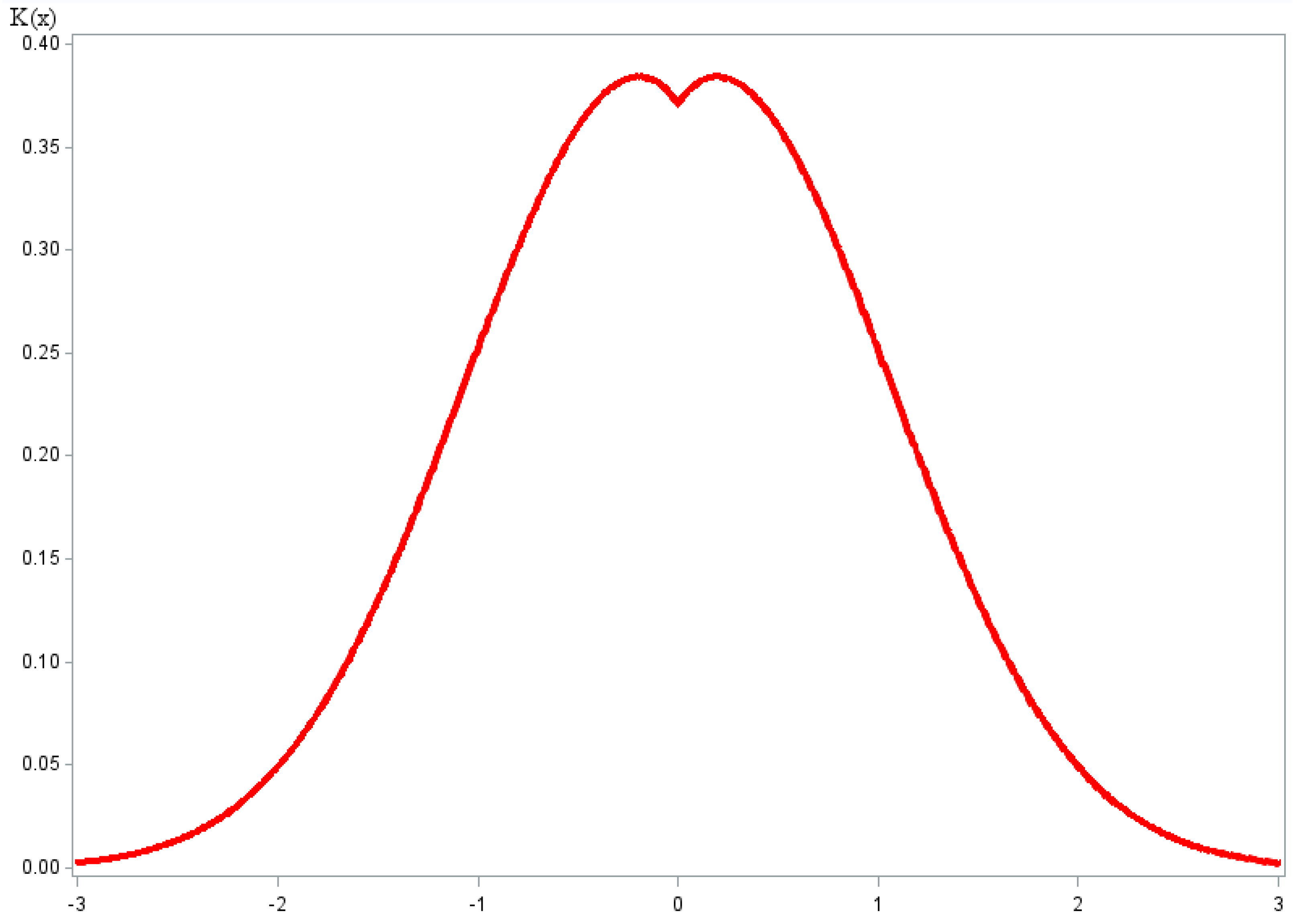
In this case, Bakshaev applied the kernel function , and we propose to apply another kernel function (Figure 1):
where.
An additional bias is introduced when the kernel function is calculated at the sample values (i.e., for ). Therefore, to eliminate this bias, the shape of the kernel function is chosen so that the influence in the environment of the sample values is as small as possible.
Let be the standard normal random variable, and be its distribution and density functions, respectively, and is an odd strictly monotonically increasing function. Then the distribution function of the random variable is , where is the inverse of the function . The distribution density of a random variable is . Let us consider the parametric class of functions , which depends on three parameters:
where is variance, is trough, and is peak shape parameter.
3. The Power of Test
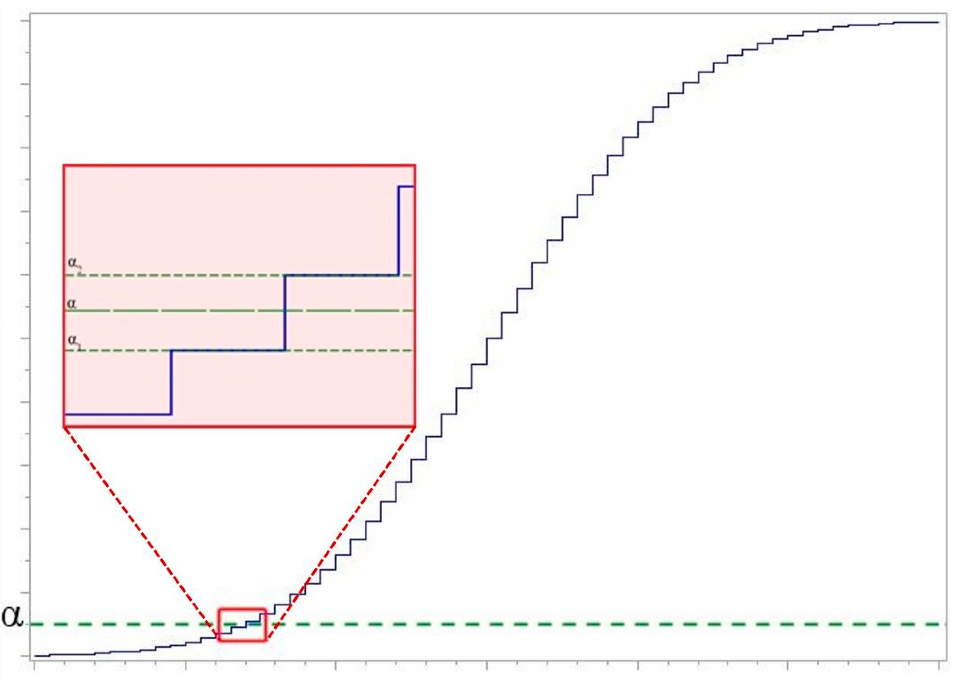
The power of the test is defined as the probability of rejecting a false hypothesis. Power is the opposite of type II error. Decreasing the probability of type I error increases the probability of type II error and decreases the power of the test. The smaller the error is, the more powerful test is. In practice, the tests are designed to minimize the type II error for a fixed type I error. The most commonly chosen value for is . The probability of the opposite event is calculated as , i.e., the power of the test (see in Figure 2) is the probability of rejecting hypothesis when it is false. The power of the test makes it possible to compare two tests significance level and sample sizes. A more powerful test has a higher value of . Increasing the sample size usually increases the power of the test [31,32].
When exact null distribution of a goodness-of-fit test statistic is a step function created by the summation of the exact probabilities for each possible value of the test statistic, it is possible to obtain the same critical value for a number of different adjacent significance levels . Linear interpolation of the power of the test statistic using the power for a significance levels (see in Figure 3) less than (denoted ) and greater than (denoted ) the desired significance level (denoted as ) is preferred by many authors to overcome this problem (see, for example, [33]). Linear interpolation gives a weighting to the power based on how close and are to . In this case, the power of the test is calculated according to the formula [19]:
where and are the critical values immediately below and above the significance level = and = are the significance levels for and , respectively.
The power of test statistics is determinate by the following steps [19]:
- The distribution of the analyzed data is formed.
- Statistics of the compatibility hypothesis test criteria are calculated. If the obtain value of statistic is greater than the corresponding critical value ( is used), then hypothesis is rejected.
- Steps 1 and 2 are repeated for (in our experiments, ) times.
- The power of a test is calculated as , where is the number of false hypotheses rejections.
4. Statistical Distributions
The simulation study considers fifteen statistical distributions for which the performance of the presented normality tests are assessed. Statistical distributions are grouped into three groups: symmetric, asymmetric, and modified normal distributions. A description of these distribution groups is presented in the following.
4.1. Symmetric Distributions
Symmetric distributions considered in this research are [20]:
- three cases of the distributionand , where and are the shape parameters;
- three cases of the distribution—, and , where and are the location and scale parameters;
- one case of the distribution, where and are the location and scale parameters;
- one case of the distribution, where and are the location and scale parameters;
- four cases of the distribution and , where is the number of degrees of freedom;
- five cases of the distribution and , where is the shape parameter; and
- one case of the standard normal distribution.
4.2. Asymmetric Distributions
Asymmetric distributions considered in this research are [20]:
- four cases of the distribution and ;
- four cases of the - distribution, and, where is the number of degrees of freedom;
- six cases of the distribution—, and , where and are the shape and scale parameters;
- one case of the distribution, where and are the location and scale parameters;
- one case of the distribution, where and are the location and scale parameters; and
- four cases of the distribution and , where and are the shape and scale parameters.
4.3. Modified Normal Distributions
Modified normal distributions considered in this research are [20]:
- six cases of the standard normal distribution truncated at and and which are referred to as NORMAL1;
- nine cases of a location-contaminated standard normal distribution, hereon termed and , which are referred to as NORMAL2;
- nine cases of a scale-contaminated standard normal distribution, hereon termed and , which are referred to as NORMAL3; and
- twelve cases of a mixture of normal distributions, hereon termed and , which are referred to as NORMAL4.
5. Simulation Study and Discussion
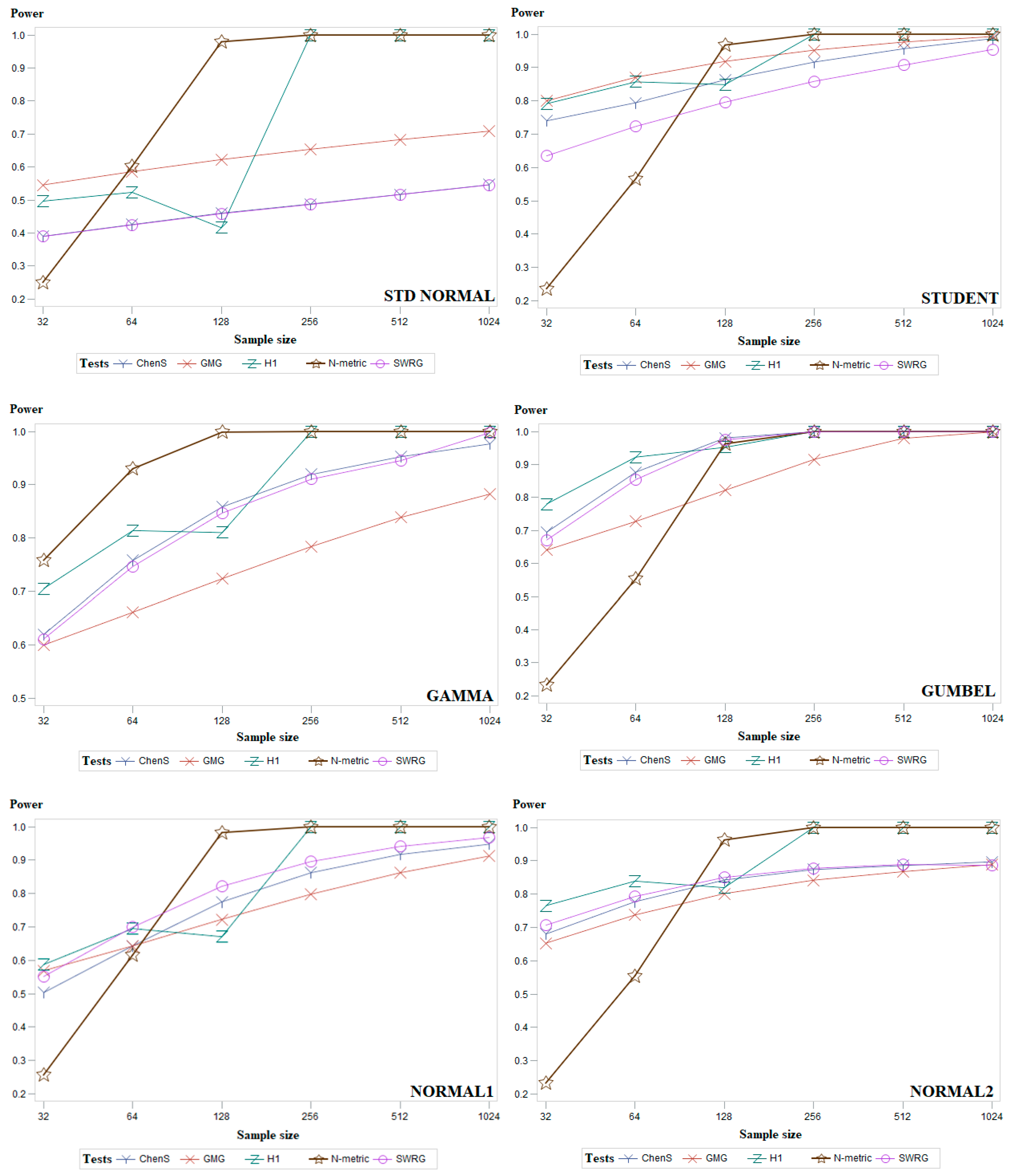
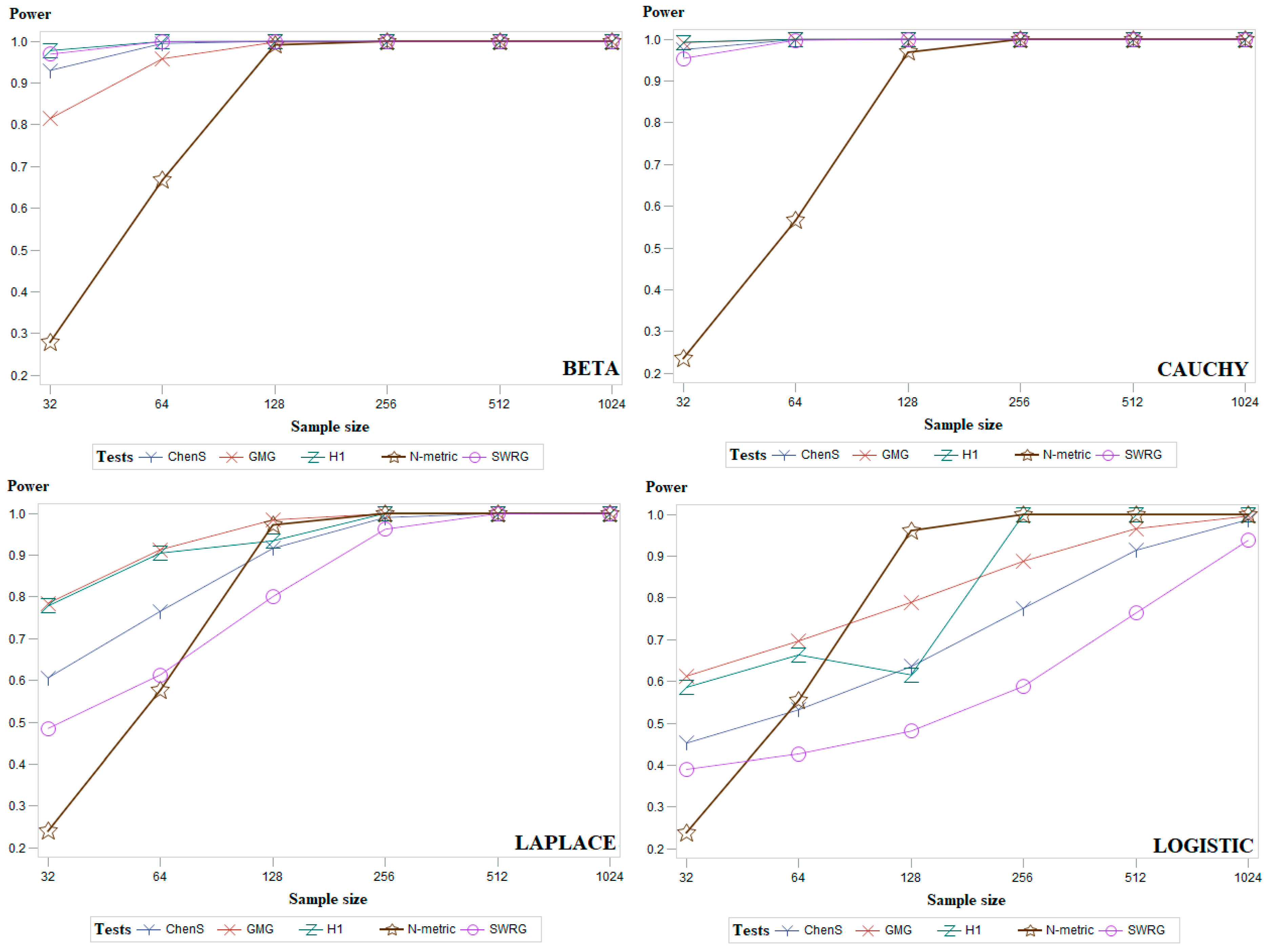
This section provides a comprehensive modeling study that is designed to evaluate the power of selected normality tests. This modeling study takes into account the effects of sample size, the level of significance () chosen, and the alternative type of distribution (Beta, Cauchy, Laplace, Logistic, Student, Chi-Square, Gamma, Gumbel, Lognormal, Weibull, and modified standard normal). The study was performed by applying 40 normality tests (including our proposed normality test) for the generated 1,000,000 standardized samples of size 32, 64, 128, 256, 512, and 1024.
The best set of parameters was selected experimentally: the value of was examined from 0.001 to 0.99 by step 0.01, the value of was examined from 0.01 to 10 by step 0.01, and the value of was examined from 0.5 to 50 by step 0.25. The N-metric test gave the most powerful results with the parameters: . In those cases, a test has several modifications, we present results only for the best variant. The Table 1, Table 2 and Table 3 present average power obtained for the symmetric, asymmetric, and modified normal distribution sets, for samples sizes of 32, 64, 128, 256, 512, and 1024. By comparing Table 1, Table 2 and Table 3, it can be seen that the most powerful test for small samples was Hosking1 (H1), the most powerful test for large sample sizes was our presented test (N-metric). According to Table 1, Table 2 and Table 3, it is observed that for large sample sizes, most tests’ power is approaching 1 except for the D’Agostino (DA) test, the power of which is significantly lower.
An additional study was conducted to determine the exact minimal sample size at which the N-metric test (statistic (34) with kernel function (35)) is the most powerful for groups of symmetric, asymmetric, and modified normal distributions. Hosking1 and N-metric tests were applied for data sets of sizes: 80, 90, 100, 105, 110, and 115. The obtained results showed that the N-metric test was the most powerful for sample size for the symmetric distributions, for sample size for the asymmetric distributions, and for sample size for a group of modified normal distributions (see in Table 4). The N-metric test is the most powerful for the Gamma distribution for sample size . It has been observed that in the case of Cauchy and Lognormal distributions, the N-metric test is the most powerful when the sample size is , which can be influenced by the long tail of these distributions.
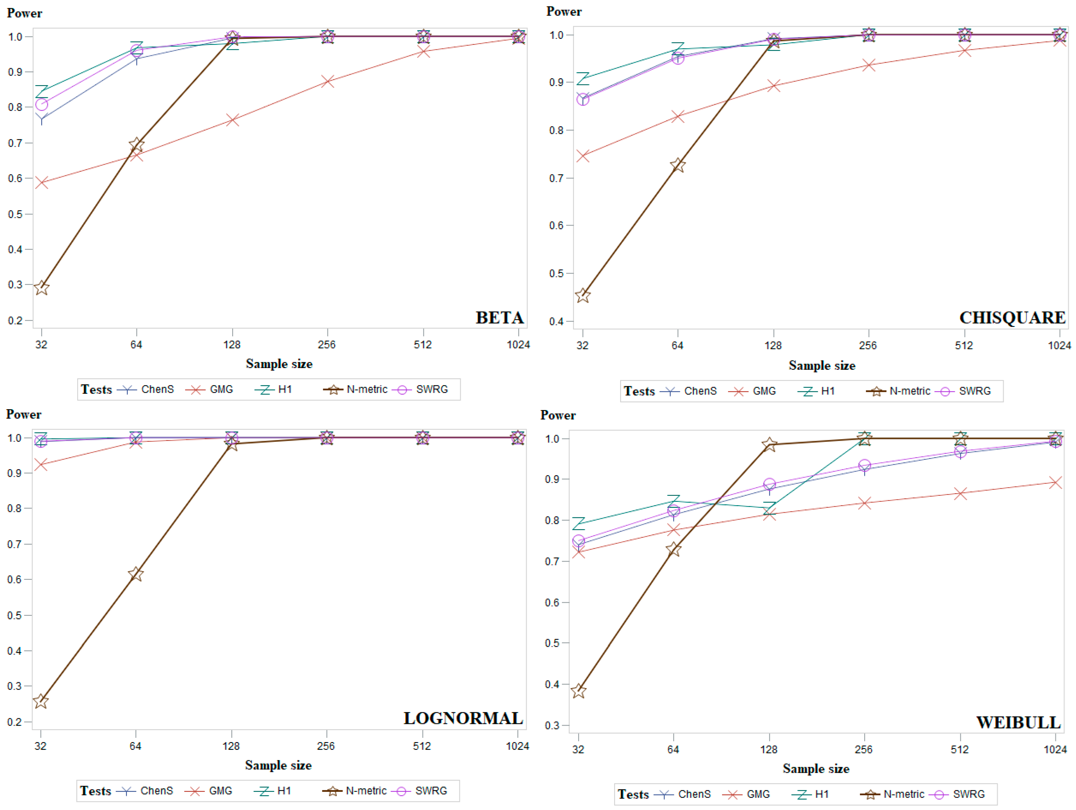
To complement the results given in Table 1, Table 2 and Table 3, Figure 4 (and Figure A1, Figure A2 and Figure A3 in Appendix A) presents the average power results of the most powerful goodness-of-fit tests. Figure 4 presents two distributions from each group of symmetric (Standard normal and Student), asymmetric (Gamma and Gumbel), and modified normal (standard normal distribution truncated at and and location-contaminated standard normal distribution) distributions. Figures of all other distributions are given in Appendix A. In Figure 4, it can be seen that for the standard normal distribution, our proposed test (N-metric) is the most powerful when the sample size is 64 or larger. Figure 4 shows that our proposed test (N-metric) is the most powerful in the case of Gamma data distribution for all sample sizes examined. In general, it can be summarized that the power of the Chen–Shapiro (ChenS), Gel–Miao–Gastwirth (GMG), Hosking1 (H1), and Modified Shapiro–Wilk (SWRG) tests increases gradually with increasing sample size. The power of our proposed test (N-metric) increases abruptly when the sample size is 128 and its power value remains close to 1 for larger sample sizes.
6. Conclusions and Future Work
In this study, a comprehensive comparison of the power of popular normality tests was performed. Given the importance of this topic and the extensive development of normality tests, the proposed new normality test, the detailed test descriptions provided, and the power comparisons are relevant. Only univariate data were examined in this study of the power of normality tests (a study with multivariate data is planned for the future).
The study addresses the performance of 40 normality tests, for various sample sizes for a number of symmetric, asymmetric, and modified normal distributions. A new goodness-of-fit test has been proposed. Its results are compared with other tests.
Based on the obtained modeling results, it was determined that the most powerful tests for the groups of symmetric, asymmetric, and modified normal distributions were Hosking1 (for smaller sample sizes) and our proposed N-metric (for larger sample sizes) test. The power of the Hosking1 test (for smaller sample sizes) is 1.5 to 7.99 percent higher than the second (by power) test for the groups of symmetric, asymmetric, and modified normal distributions. The power of the N-metric test (for larger sample sizes) is 6.2 to 16.26 percent higher than the second (by power) test for the groups of symmetric, asymmetric, and modified normal distributions.
The N-metric test is recommended to be used for symmetric data sets of size , for asymmetric data sets of size , and for bell-shaped distributed data sets of size .
Author Contributions
Data curation, J.A. and T.R.; formal analysis, J.A. and T.R.; investigation, J.A. and T.R.; methodology, J.A. and T.R.; software, J.A. and T.R.; supervision, T.R.; writing—original draft, J.A. and M.B.; writing—review and editing, J.A. and M.B. All authors have read and agreed to the published version of the manuscript.
Funding
This research received no external funding.
Institutional Review Board Statement
Not applicable.
Informed Consent Statement
Not applicable.
Data Availability Statement
Generated data sets were used in the study (see in Section 4).
Conflicts of Interest
The authors declare no conflict of interest.
Appendix A
Figure A1.
Average empirical power results, for all sample sizes, for the groups of symmetric distributions of five powerful goodness-of-fit tests.
Figure A1.
Average empirical power results, for all sample sizes, for the groups of symmetric distributions of five powerful goodness-of-fit tests.

Figure A2.
Average empirical power results for the examined sample sizes for the groups of asymmetric distributions of five powerful goodness-of-fit tests.
Figure A2.
Average empirical power results for the examined sample sizes for the groups of asymmetric distributions of five powerful goodness-of-fit tests.

Figure A3.
Average empirical power results for the examined sample sizes for the groups of the modified normal distributions of five powerful goodness-of-fit tests.
Figure A3.
Average empirical power results for the examined sample sizes for the groups of the modified normal distributions of five powerful goodness-of-fit tests.

References
- Barnard, G.A.; Barnard, G.A. Introduction to Pearson (1900) on the Criterion That a Given System of Deviations from the Probable in the Case of a Correlated System of Variables is Such That it Can be Reasonably Supposed to Have Arisen from Random Sampling; Springer Series in Statistics Breakthroughs in Statistics; Springer: Cham, Switzerland, 1992; pp. 1–10. [Google Scholar]
- Kolmogorov, A. Sulla determinazione empirica di una legge di distribuzione. Inst. Ital. Attuari Giorn. 1933, 4, 83–91. [Google Scholar]
- Adefisoye, J.; Golam Kibria, B.; George, F. Performances of several univariate tests of normality: An empirical study. J. Biom. Biostat. 2016, 7, 1–8. [Google Scholar]
- Anderson, T.W.; Darling, D.A. Asymptotic theory of certain “goodness-of-fit” criteria based on stochastic processes. Ann. Math. Stat. 1952, 23, 193–212. [Google Scholar] [CrossRef]
- Hosking, J.R.M.; Wallis, J.R. Some statistics useful in regional frequency analysis. Water Resour. Res. 1993, 29, 271–281. [Google Scholar] [CrossRef]
- Cabana, A.; Cabana, E.M. Goodness-of-Fit and Comparison Tests of the Kolmogorov-Smirnov Type for Bivariate Populations. Ann. Stat. 1994, 22, 1447–1459. [Google Scholar] [CrossRef]
- Chen, L.; Shapiro, S.S. An Alternative Test for Normality Based on Normalized Spacings. J. Stat. Comput. Simul. 1995, 53, 269–288. [Google Scholar] [CrossRef]
- Rahman, M.M.; Govindarajulu, Z. A modification of the test of Shapiro and Wilk for normality. J. Appl. Stat. 1997, 24, 219–236. [Google Scholar] [CrossRef]
- Ray, W.D.; Shenton, L.R.; Bowman, K.O. Maximum Likelihood Estimation in Small Samples. J. R. Stat. Soc. Ser. A 1978, 141, 268. [Google Scholar] [CrossRef]
- Zhang, P. Omnibus test of normality using the Q statistic. J. Appl. Stat. 1999, 26, 519–528. [Google Scholar] [CrossRef]
- Barrio, E.; Cuesta-Albertos, J.A.; Matrán, C.; Rodríguez-Rodríguez, J.M. Tests of goodness of fit based on the L2-Wasserstein distance. Ann. Stat. 1999, 27, 1230–1239. [Google Scholar]
- Glen, A.G.; Leemis, L.M.; Barr, D.R. Order statistics in goodness-of-fit testing. IEEE Trans. Reliab. 2001, 50, 209–213. [Google Scholar] [CrossRef]
- Bonett, D.G.; Seier, E. A test of normality with high uniform power. Comput. Stat. Data Anal. 2002, 40, 435–445. [Google Scholar] [CrossRef]
- Psaradakis, Z.; Vávra, M. Normality tests for dependent data: Large-sample and bootstrap approaches. Commun. Stat.-Simul. Comput. 2018, 49, 283–304. [Google Scholar] [CrossRef] [Green Version]
- Zhang, J.; Wu, Y. Likelihood-ratio tests for normality. Comput. Stat. Data Anal. 2005, 49, 709–721. [Google Scholar] [CrossRef]
- Gel, Y.R.; Miao, W.; Gastwirth, J.L. Robust directed tests of normality against heavy-tailed alternatives. Comput. Stat. Data Anal. 2007, 51, 2734–2746. [Google Scholar] [CrossRef]
- Coin, D. A goodness-of-fit test for normality based on polynomial regression. Comput. Stat. Data Anal. 2008, 52, 2185–2198. [Google Scholar] [CrossRef]
- Desgagné, A.; Lafaye de Micheaux, P. A powerful and interpretable alternative to the Jarque–Bera test of normality based on 2nd-power skewness and kurtosis, using the Rao’s score test on the APD family. J. Appl. Stat. 2017, 45, 2307–2327. [Google Scholar] [CrossRef]
- Steele, C.M. The Power of Categorical Goodness-Of-Fit Statistics. Ph.D. Thesis, Australian School of Environmental Studies, Warrandyte, Victoria, Australia, 2003. [Google Scholar]
- Romão, X.; Delgado, R.; Costa, A. An empirical power comparison of univariate goodness-of-fit tests for normality. J. Stat. Comput. Simul. 2010, 80, 545–591. [Google Scholar] [CrossRef]
- Choulakian, V.; Lockhart, R.; Stephens, M. Cramérvon Mises statistics for discrete distributions. Can. J. Stat. 1994, 22, 125–137. [Google Scholar] [CrossRef]
- Shapiro, S.S.; Wilk, M.B. An analysis of variance test for normality (complete samples). Biometrika 1965, 52, 591–611. [Google Scholar] [CrossRef]
- Lilliefors, H.W. On the Kolmogorov-Smirnov test for normality with mean and variance unknown. J. Am. Stat. Assoc. 1967, 62, 399–402. [Google Scholar] [CrossRef]
- Ahmad, F.; Khan, R.A. A power comparison of various normality tests. Pak. J. Stat. Oper. Res. 2015, 11, 331. [Google Scholar] [CrossRef] [Green Version]
- D’Agostino, R.B.; Pearson, E.S. Testing for departures from normality. I. Fuller empirical results for the distribution of b2 and √b1. Biometrika 1973, 60, 613–622. [Google Scholar]
- Filliben, J.J. The Probability Plot Correlation Coefficient Test for Normality. Technometrics 1975, 17, 111–117. [Google Scholar] [CrossRef]
- Martinez, J.; Iglewicz, B. A test for departure from normality based on a biweight estimator of scale. Biometrika 1981, 68, 331–333. [Google Scholar] [CrossRef]
- Epps, T.W.; Pulley, L.B. A test for normality based on the empirical characteristic function. Biometrika 1983, 70, 723–726. [Google Scholar] [CrossRef]
- Jarque, C.; Bera, A. Efficient tests for normality, homoscedasticity andserial independence of regression residuals. Econ. Lett. 1980, 6, 255–259. [Google Scholar] [CrossRef]
- Bakshaev, A. Goodness of fit and homogeneity tests on the basis of N-distances. J. Stat. Plan. Inference 2009, 139, 3750–3758. [Google Scholar] [CrossRef]
- Hill, T.; Lewicki, P. Statistics Methods and Applications; StatSoft: Tulsa, OK, USA, 2007. [Google Scholar]
- Kasiulevičius, V.; Denapienė, G. Statistikos taikymas mokslinių tyrimų analizėje. Gerontologija 2008, 9, 176–180. [Google Scholar]
- Damianou, C.; Kemp, A.W. New goodness of statistics for discrete and continuous data. Am. J. Math. Manag. Sci. 1990, 10, 275–307. [Google Scholar]
Figure 1.
Plot of out kernel function with experimentally chosen optimal parameters .

Figure 2.
Illustration of the power.

Figure 3.
Significance levels of the statistic step function.

Figure 4.
Average empirical power results, for the examined sample sizes, for the groups of symmetric, asymmetric, and modified normal distributions of five powerful goodness-of-fit tests.
Figure 4.
Average empirical power results, for the examined sample sizes, for the groups of symmetric, asymmetric, and modified normal distributions of five powerful goodness-of-fit tests.


Table 1.
Average empirical power obtained for a group of symmetric distributions.
| Sample Size | |||||||
|---|---|---|---|---|---|---|---|
| 32 | 64 | 128 | 256 | 512 | 1024 | ||
| Tests | AD | 0.714 | 0.799 | 0.863 | 0.909 | 0.939 | 0.955 |
| BCMR | 0.718 | 0.809 | 0.875 | 0.920 | 0.947 | 0.947 | |
| BHS | 0.431 | 0.551 | 0.663 | 0.752 | 0.818 | 0.868 | |
| BHSBS | 0.680 | 0.778 | 0.783 | 0.903 | 0.938 | 0.959 | |
| BM2 | 0.726 | 0.835 | 0.905 | 0.945 | 0.965 | 0.974 | |
| BS | 0.717 | 0.810 | 0.877 | 0.920 | 0.947 | 0.961 | |
| CC2 | 0.712 | 0.805 | 0.873 | 0.920 | 0.949 | 0.936 | |
| CHI2 | 0.663 | 0.778 | 0.842 | 0.884 | 0.941 | 0.945 | |
| CVM | 0.591 | 0.733 | 0.805 | 0.855 | 0.919 | 0.949 | |
| ChenS | 0.729 | 0.806 | 0.871 | 0.915 | 0.943 | 0.960 | |
| Coin | 0.735 | 0.830 | 0.891 | 0.930 | 0.952 | 0.963 | |
| DA | 0.266 | 0.295 | 0.314 | 0.319 | 0.315 | 0.311 | |
| DAP | 0.723 | 0.820 | 0.883 | 0.924 | 0.948 | 0.962 | |
| DH | 0.709 | 0.805 | 0.877 | 0.925 | 0.950 | 0.963 | |
| DLDMZEPD | 0.730 | 0.826 | 0.889 | 0.929 | 0.952 | 0.963 | |
| EP | 0.706 | 0.828 | 0.974 | 0.910 | 0.946 | 0.959 | |
| Filli | 0.712 | 0.805 | 0.875 | 0.922 | 0.949 | 0.962 | |
| GG | 0.658 | 0.760 | 0.850 | 0.915 | 0.949 | 0.962 | |
| GLB | 0.712 | 0.798 | 0.863 | 0.909 | 0.943 | 0.918 | |
| GMG | 0.787 | 0.862 | 0.914 | 0.946 | 0.965 | 0.975 | |
| H1 | 0.799 | 0.862 | 0.852 | 0.999 | 0.999 | 0.999 | |
| JB | 0.643 | 0.762 | 0.856 | 0.918 | 0.949 | 0.963 | |
| KS | 0.585 | 0.723 | 0.789 | 0.836 | 0.905 | 0.939 | |
| Lillie | 0.669 | 0.758 | 0.828 | 0.883 | 0.921 | 0.947 | |
| MI | 0.632 | 0.676 | 0.705 | 0.724 | 0.736 | 0.745 | |
| N-metric | 0.245 | 0.585 | 0.971 | 0.999 | 0.999 | 0.999 | |
| SF | 0.715 | 0.807 | 0.876 | 0.923 | 0.949 | 0.962 | |
| SW | 0.718 | 0.808 | 0.874 | 0.919 | 0.946 | 0.962 | |
| SWRG | 0.694 | 0.775 | 0.834 | 0.882 | 0.916 | 0.946 | |
| ZQstar | 0.513 | 0.576 | 0.630 | 0.669 | 0.697 | 0.718 | |
| ZW2 | 0.715 | 0.806 | 0.869 | 0.912 | 0.939 | 0.957 | |
Table 2.
Average empirical power obtained for a group of asymmetric distributions.
| Sample Size | |||||||
|---|---|---|---|---|---|---|---|
| 32 | 64 | 128 | 256 | 512 | 1024 | ||
| Tests | AD | 0.729 | 0.835 | 0.908 | 0.949 | 0.969 | 0.984 |
| BCMR | 0.749 | 0.856 | 0.924 | 0.971 | 0.995 | 0.991 | |
| BHS | 0.529 | 0.664 | 0.769 | 0.855 | 0.915 | 0.950 | |
| BHSBS | 0.538 | 0.652 | 0.747 | 0.914 | 0.902 | 0.944 | |
| BM2 | 0.737 | 0.859 | 0.931 | 0.965 | 0.981 | 0.993 | |
| BS | 0.506 | 0.588 | 0.665 | 0.738 | 0.805 | 0.859 | |
| CC2 | 0.579 | 0.682 | 0.777 | 0.853 | 0.938 | 0.956 | |
| CHI2 | 0.645 | 0.799 | 0.881 | 0.934 | 0.965 | 0.980 | |
| CVM | 0.594 | 0.755 | 0.836 | 0.887 | 0.935 | 0.957 | |
| ChenS | 0.756 | 0.862 | 0.928 | 0.961 | 0.978 | 0.991 | |
| Coin | 0.480 | 0.556 | 0.630 | 0.700 | 0.769 | 0.916 | |
| DA | 0.237 | 0.223 | 0.209 | 0.198 | 0.191 | 0.192 | |
| DAP | 0.705 | 0.826 | 0.910 | 0.955 | 0.977 | 0.990 | |
| DH | 0.724 | 0.845 | 0.921 | 0.957 | 0.977 | 0.991 | |
| DLDMXAPD | 0.726 | 0.843 | 0.918 | 0.955 | 0.975 | 0.989 | |
| EP | 0.753 | 0.846 | 0.913 | 0.967 | 0.975 | 0.993 | |
| Filli | 0.732 | 0.842 | 0.915 | 0.953 | 0.974 | 0.991 | |
| GG | 0.672 | 0.805 | 0.898 | 0.949 | 0.973 | 0.988 | |
| GLB | 0.725 | 0.831 | 0.905 | 0.987 | 0.970 | 0.984 | |
| GMG | 0.683 | 0.751 | 0.809 | 0.859 | 0.901 | 0.932 | |
| H1 | 0.816 | 0.896 | 0.896 | 0.999 | 0.999 | 0.999 | |
| JB | 0.662 | 0.808 | 0.904 | 0.953 | 0.975 | 0.989 | |
| KS | 0.582 | 0.736 | 0.810 | 0.863 | 0.921 | 0.945 | |
| Lillie | 0.671 | 0.786 | 0.872 | 0.929 | 0.959 | 0.976 | |
| MI | 0.644 | 0.731 | 0.798 | 0.843 | 0.872 | 0.913 | |
| N-metric | 0.464 | 0.761 | 0.990 | 0.999 | 0.999 | 0.999 | |
| SF | 0.736 | 0.846 | 0.918 | 0.955 | 0.975 | 0.989 | |
| SW | 0.753 | 0.859 | 0.925 | 0.959 | 0.977 | 0.991 | |
| SWRG | 0.758 | 0.861 | 0.927 | 0.960 | 0.977 | 0.999 | |
| ZQstar | 0.570 | 0.639 | 0.693 | 0.732 | 0.761 | 0.748 | |
| ZW2 | 0.764 | 0.870 | 0.932 | 0.962 | 0.980 | 0.997 | |
Table 3.
Average empirical power obtained for a group of modified normal distributions.
| Sample Size | |||||||
|---|---|---|---|---|---|---|---|
| 32 | 64 | 128 | 256 | 512 | 1024 | ||
| Tests | AD | 0.662 | 0.756 | 0.825 | 0.872 | 0.905 | 0.931 |
| BCMR | 0.652 | 0.756 | 0.831 | 0.880 | 0.913 | 0.935 | |
| BHS | 0.463 | 0.585 | 0.676 | 0.744 | 0.796 | 0.834 | |
| BHSBS | 0.568 | 0.701 | 0.787 | 0.847 | 0.890 | 0.918 | |
| BM2 | 0.641 | 0.770 | 0.854 | 0.904 | 0.934 | 0.953 | |
| BS | 0.587 | 0.688 | 0.770 | 0.833 | 0.881 | 0.916 | |
| CC2 | 0.576 | 0.675 | 0.763 | 0.833 | 0.887 | 0.923 | |
| CHI2 | 0.566 | 0.728 | 0.808 | 0.866 | 0.914 | 0.939 | |
| CVM | 0.557 | 0.708 | 0.779 | 0.833 | 0.897 | 0.930 | |
| ChenS | 0.656 | 0.759 | 0.833 | 0.882 | 0.915 | 0.937 | |
| Coin | 0.579 | 0.691 | 0.781 | 0.846 | 0.889 | 0.918 | |
| DA | 0.314 | 0.342 | 0.367 | 0.388 | 0.405 | 0.418 | |
| DAP | 0.617 | 0.733 | 0.818 | 0.872 | 0.906 | 0.930 | |
| DH | 0.617 | 0.727 | 0.815 | 0.872 | 0.907 | 0.930 | |
| DLDMXAPD | 0.651 | 0.754 | 0.831 | 0.879 | 0.912 | 0.935 | |
| EP | 0.640 | 0.748 | 0.819 | 0.865 | 0.906 | 0.931 | |
| Filli | 0.637 | 0.743 | 0.823 | 0.877 | 0.911 | 0.933 | |
| GG | 0.529 | 0.657 | 0.775 | 0.860 | 0.906 | 0.932 | |
| GLB | 0.659 | 0.755 | 0.823 | 0.870 | 0.903 | 0.930 | |
| GMG | 0.688 | 0.771 | 0.836 | 0.883 | 0.917 | 0.942 | |
| H1 | 0.743 | 0.816 | 0.799 | 0.999 | 0.999 | 0.999 | |
| JB | 0.515 | 0.662 | 0.783 | 0.861 | 0.904 | 0.930 | |
| KS | 0.564 | 0.710 | 0.772 | 0.825 | 0.893 | 0.924 | |
| Lillie | 0.626 | 0.724 | 0.796 | 0.850 | 0.889 | 0.917 | |
| MI | 0.494 | 0.536 | 0.563 | 0.578 | 0.585 | 0.590 | |
| N-metric | 0.243 | 0.582 | 0.972 | 0.999 | 0.999 | 0.999 | |
| SF | 0.642 | 0.747 | 0.826 | 0.879 | 0.912 | 0.934 | |
| SW | 0.654 | 0.758 | 0.832 | 0.882 | 0.915 | 0.937 | |
| SWRG | 0.643 | 0.746 | 0.818 | 0.864 | 0.901 | 0.931 | |
| ZQstar | 0.394 | 0.423 | 0.450 | 0.472 | 0.487 | 0.498 | |
| ZW2 | 0.640 | 0.749 | 0.826 | 0.876 | 0.907 | 0.931 | |
Table 4.
The minimal sample size at which the N-metric test is most powerful.
| Nr. | Distribution | Groups of Distributions | |
|---|---|---|---|
| 1. | Standard normal | Symmetric | 46 |
| 2. | Beta | Symmetric | 88 |
| 3. | Cauchy | Symmetric | 257 |
| 4. | Laplace | Symmetric | 117 |
| 5. | Logistic | Symmetric | 71 |
| 6. | Student | Symmetric | 96 |
| 7. | Beta | Asymmetric | 108 |
| 8. | Chi-square | Asymmetric | 123 |
| 9. | Gamma | Asymmetric | <32 |
| 10. | Gumbel | Asymmetric | 125 |
| 11. | Lognormal | Asymmetric | 255 |
| 12. | Weibull | Asymmetric | 65 |
| 13. | Normal1 | Modified normal | 70 |
| 14. | Normal2 | Modified normal | 93 |
| 15. | Normal3 | Modified normal | 72 |
| 16. | Normal4 | Modified normal | 117 |
Publisher’s Note: MDPI stays neutral with regard to jurisdictional claims in published maps and institutional affiliations. |
© 2021 by the authors. Licensee MDPI, Basel, Switzerland. This article is an open access article distributed under the terms and conditions of the Creative Commons Attribution (CC BY) license (https://creativecommons.org/licenses/by/4.0/).
Share and Cite
MDPI and ACS Style
Arnastauskaitė, J.; Ruzgas, T.; Bražėnas, M. An Exhaustive Power Comparison of Normality Tests. Mathematics 2021, 9, 788. https://doi.org/10.3390/math9070788
AMA Style
Arnastauskaitė J, Ruzgas T, Bražėnas M. An Exhaustive Power Comparison of Normality Tests. Mathematics. 2021; 9(7):788. https://doi.org/10.3390/math9070788
Chicago/Turabian StyleArnastauskaitė, Jurgita, Tomas Ruzgas, and Mindaugas Bražėnas. 2021. "An Exhaustive Power Comparison of Normality Tests" Mathematics 9, no. 7: 788. https://doi.org/10.3390/math9070788
Note that from the first issue of 2016, this journal uses article numbers instead of page numbers. See further details here.