F-Operators for the Construction of Closed Form Solutions to Linear Homogenous PDEs with Variable Coefficients

Abstract

A computational framework for the construction of solutions to linear homogenous partial differential equations (PDEs) with variable coefficients is developed in this paper. The considered class of PDEs reads: $\frac{\partial p}{\partial t}-{\sum }_{j=0}^m\left({\sum }_{r=0}^{n_j}{a}_{jr}\left(t\right)x^r\right)\frac{\partial j_p}{\partial x^j}=0$ F-operators are introduced and used to transform the original PDE into the image PDE. Factorization of the solution into rational and exponential parts enables us to construct analytic solutions without direct integrations. A number of computational examples are used to demonstrate the efficiency of the proposed scheme.

1. Introduction

The Fourier transform, as one of the most important concepts in signal analysis, is widely used for the construction of solutions to partial differential equations (PDEs). While there exist numerous classical techniques for the construction of solutions to PDEs based on the Fourier transform, recent research demonstrates that new approaches in this field remain an important area of investigation.

The immersed boundary smooth extension method for solving PDEs in general domains is presented in [1]. This high-order accuracy numerical scheme smoothly extends the unknown solution of the PDE from a given smooth domain to a larger computational domain, enabling the use of Fourier spectral methods. Local fractional Fourier transform operator via Mittag–Leffler function defined on the fractal set is used to solve PDEs in [2]. An efficient computational scheme based on a Laplace transform-based exponential time integrator combined with a flexible Krylov subspace approach is proposed in [3] to solve linear, time-dependent, parabolic PDEs. Fourier wavelets are used to construct solutions to partial differential equations in [4].

Fractional higher-order Fourier transform method is proposed to solve fractional reaction-diffusion PDE problems in [5]. The Fourier pseudospectral method is used for developing new structure-preserving algorithms for general multi-symplectic formulations of Hamiltonian PDEs in [6]. The modified homotopy perturbation method, combined with the Fourier transform, is used to solve the nonlinear and singular Lane–Emden PDE equations in [7]. Analytical solutions to the fractional heat diffusion, fractional wave, fractional telegraph and fractional kinetic equations are obtained via the fractional Fourier transform in [8]. A Crank–Nicholson scheme of a Fourier pseudospectral method is applied to the fractional stationary Schrödinger equation in [9].

The derivative of the solution to linear elliptic PDEs, perpendicularly to the direction of an arbitrary angle to the boundary, is computed without solving on the interior of the domain in [10]. The deployment of the FFT for the solution of the associated collocation linear system yields significant computational savings in [10]. Algorithm for approximate reconstruction of transient heating curves from sparse frequency domain data by using modified inverse Fourier transform is developed in [11]. A conservative Fourier spectral scheme is presented for higher order Klein–Gordon–Schrödinger system with periodic boundary conditions in [12,13].

Efficient numerical Fourier methods for coupled forward-backward stochastic DEs are developed in [14]. The generalized Fourier transform is used for reducing the computational cost and memory requirements of radial basis function methods for multi-dimensional option pricing in [15]. A general algorithm, including a transformation of the Black–Scholes equation into the heat equation, that can be used in any number of dimensions is also developed in [15].

In this paper, a scheme for the construction of analytic solutions to linear homogenous PDEs with variable coefficients is proposed. The scheme is based on F-operators that enable the realization of the Fourier transform without direct integration. Derived operators are used to transform the original PDEs into image PDEs. Generalized Gaussian analytic solutions that are factored into rational and exponential parts are considered. Application of the F-operator scheme enables the construction of analytical solutions without direct integration of the original PDE.

The paper is organized as follows. Section 2 contains the necessary preliminary definitions and introduces F-operators. Main results on the realization of the Fourier transform using F-operators are given in Section 3. A scheme for the construction of analytic solutions to homogenous linear PDEs with variable coefficients is derived in Section 4. Section 5 contains computational examples that demonstrate the efficiency of the proposed scheme. Section 6 contains concluding remarks.

2. Preliminaries

2.1. Generalized Gaussian Functions

Definition 1.

The linear operators

$${\mathbf{F}}_t:=i\left(tx-{\mathbf{D}}_x\right),{\widehat{\mathbf{F}}}_t:=i\left({\mathbf{D}}_x-\frac{x}{t}\right),$$

(1)

where ${\mathbf{D}}_x$ is the directional derivative operator with respect to x and $i^2=-1$ are called forward and backward F-operators, respectively.

In the following computation, powers of the operators ${\mathbf{F}}_t$ and ${\widehat{\mathbf{F}}}_t$ are applied to the unit. The results read:

$$\begin{array}{cc}\hfill & {\mathbf{F}}_t^{0}1=1,{\mathbf{F}}_{t}1=itx,{\mathbf{F}}_t^{2}1={\mathbf{F}}_{t}itx=t-t^2{x}^2,\dots ;\hfill \end{array}$$

(2)

$$\begin{array}{cc}\hfill & {\widehat{\mathbf{F}}}_t^{0}1=1,{\widehat{\mathbf{F}}}_{t}1=-\frac{ix}{t},{\widehat{\mathbf{F}}}_t^{2}1={\widehat{\mathbf{F}}}_t\left(-\frac{ix}{t}\right)=\frac{1}{t}-\frac{x^2}{t^2},\dots .\hfill \end{array}$$

(3)

Note that ${\mathbf{F}}_t^{j}1$ can be expressed in terms of Hermite polynomials [16]:

$${\mathbf{F}}_t^{j}1=i^j{t}^{\frac{j}{2}}H{e}_j\left(\sqrt{t}x\right),j=0,1,\dots$$

(4)

where $H{e}_j\left(x\right),j=0,1,\dots$ are probabilistic Hermite polynomials.

Definition 2.

Consider the following set of rational functions:

$${\mathbb{M}}_t=\left\{\frac{{\sum }_{k=0}^m{\alpha }_k{t}^k}{{\sum }_{l=0}^n{\beta }_l{t}^l}|m,n\in {\mathbb{Z}}_0;{\alpha }_k,{\beta }_l\in \mathbb{C};t\in \mathbb{R}\right\}.$$

(5)

The function $Q(x,t)$ is a carrier polynomial in x, defined as:

$$Q(x,t)=\sum _{j=0}^r{a}_j\left(t\right)x^j,$$

(6)

where

$$a_j\left(t\right)\in {\mathbb{M}}_t,j=0,1,\dots .$$

(7)

The image $\widehat{Q}(x,t)$ of the carrier polynomial $Q(x,t)$ can be constructed using (6) and (2):

$$\widehat{Q}(x,t):=Q\left({\mathbf{F}}_t,t\right)1=\sum _{j=0}^r{a}_j\left(t\right)\left({\mathbf{F}}_t^{j}1\right)=\sum _{j=0}^r{\widehat{a}}_j\left(t\right)x^j.$$

(8)

Definition 3.

The generalized Gaussian function $p=p(x,t)$ is defined as:

$$p(x,t)=\frac{1}{\sqrt{2\pi t}}Q(x,t)exp\left(-\frac{x^2}{2t}\right).$$

(9)

For brevity, the notation $p_0(x,t)=\frac{1}{\sqrt{2\pi t}}exp\left(-\frac{x^2}{2t}\right)$ will be used further.

2.2. The Fourier Transform—Classical Formulas

For any generalized Gaussian function $p(x,t)$, the Fourier transform yields the image $\widehat{p}(x,t)$:

$$\widehat{p}(x,t)=\mathcal{F}\left(p\right)={\int }_{-\infty }^{+\infty }exp\left(ixy\right)p(y,t)\mathrm{dy}.$$

(10)

The inverse transform reads:

$$p(x,t)={\mathcal{F}}^{-1}\left(\widehat{p}\right)=\frac{1}{2\pi }{\int }_{-\infty }^{+\infty }exp\left(-ixy\right)\widehat{p}(y,t)\mathrm{dy}.$$

(11)

Note that:

$${\widehat{p}}_0(x,t)=\mathcal{F}\left(p_0\right)=exp\left(-\frac{t{x}^2}{2}\right).$$

(12)

The following equalities do hold:

$$\begin{array}{cc}\hfill & \mathcal{F}\left(xp\right)=-i{\mathbf{D}}_x\mathcal{F}\left(p\right),\mathcal{F}\left({\mathbf{D}}_{x}p\right)=-ix\mathcal{F}\left(p\right);\hfill \end{array}$$

(13)

$$\begin{array}{cc}\hfill & {\mathcal{F}}^{-1}\left(x\widehat{p}\right)=i{\mathbf{D}}_x{\mathcal{F}}^{-1}\left(\widehat{p}\right),{\mathcal{F}}^{-1}\left({\mathbf{D}}_x\widehat{p}\right)=ix{\mathcal{F}}^{-1}\left(\widehat{p}\right);\hfill \end{array}$$

(14)

$$\begin{array}{cc}\hfill & \mathcal{F}\left(tp\right)=t\mathcal{F}\left(p\right),\mathcal{F}\left({\mathbf{D}}_{t}p\right)={\mathbf{D}}_t\mathcal{F}\left(p\right);\hfill \end{array}$$

(15)

$$\begin{array}{cc}\hfill & {\mathcal{F}}^{-1}\left(t\widehat{p}\right)=t{\mathcal{F}}^{-1}\left(\widehat{p}\right),{\mathcal{F}}^{-1}\left({\mathbf{D}}_t\widehat{p}\right)={\mathbf{D}}_t{\mathcal{F}}^{-1}\left(\widehat{p}\right).\hfill \end{array}$$

(16)

3. Main Results

The Fourier transform of generalized Gaussian functions is considered in this section. It is shown that the Fourier transform can be realized using the forward and backward F-operators (1) and that it is enough to consider the action of (1) on the carrier polynomials $Q(x,t),\widehat{Q}(x,t)$.

3.1. The Fourier Transform of the Generalized Gaussian Function

Theorem 1.

The Fourier transform of the generalized Gaussian function $p=p(x,t)$ has the following form:

$$\widehat{p}(x,t)=\widehat{Q}(x,t){\widehat{p}}_0(x,t),$$

(17)

where $\widehat{Q}(x,t)=Q\left({\mathbf{F}}_t,t\right)1$.

Proof. 

The theorem is proved using mathematical induction.

Let $Q_n\left(x\right):=x^n,n=0,1,\dots$ and $p_n(x,t):=Q_n\left(x\right)p_0(x,t)$. The Fourier transform of $p_n$ reads:

$$\begin{array}{cc}\hfill \mathcal{F}\left(p_n\right)& ={\int }_{-\infty }^{+\infty }exp\left(ixy\right)y^n{p}_0(y,t)\mathrm{dy}={\left(-i{\mathbf{D}}_x\right)}^n{\int }_{-\infty }^{+\infty }exp\left(ixy\right)p_0(y,t)\mathrm{dy}\hfill \\ \hfill & ={\left(-i{\mathbf{D}}_x\right)}^n{\widehat{p}}_0(x,t).\hfill \end{array}$$

(18)

For $n=0$, the theorem holds true. Taking $n=1$ yields:

$$\begin{array}{cc}\hfill \mathcal{F}\left(x{p}_0\right)& =\left(-i{\mathbf{D}}_x\right)exp\left(-\frac{t{x}^2}{2}\right)=itxexp\left(-\frac{t{x}^2}{2}\right)=\left(i\left(tx-{\mathbf{D}}_x\right)1\right){\widehat{p}}_0(x,t)\hfill \\ \hfill & =\left({\mathbf{F}}_{t}1\right){\widehat{p}}_0(x,t).\hfill \end{array}$$

(19)

Let us denote ${\widehat{Q}}_n\left(x,t\right):={\mathbf{F}}_t^{n}1,n=2,3,\dots$. Suppose that equalities

$${\widehat{p}}_k(x,t)={\widehat{Q}}_k\left(x,t\right){\widehat{p}}_0(x,t),k=1,2,\dots ,n,$$

(20)

hold true. Then the Fourier transform of $p_{n+1}(x,t)$ reads:

$$\begin{array}{cc}\hfill \mathcal{F}\left(x^{n+1}{p}_0\right)& ={\left(-i{\mathbf{D}}_x\right)}^{n+1}{\widehat{p}}_0(x,t)=-i{\mathbf{D}}_x\left({\left(-i{\mathbf{D}}_x\right)}^n{p}_0(x,t)\right)\hfill \\ & =-i{\mathbf{D}}_x\left({\widehat{Q}}_n\left(x,t\right){\widehat{p}}_0(x,t)\right)\hfill \\ \hfill & =-i\left(\left({\mathbf{D}}_x{\widehat{Q}}_n(x,t)\right){\widehat{p}}_0(x,t)-tx{\widehat{Q}}_n(x,t){\widehat{p}}_0(x,t)\right)=\hfill \\ \hfill & =\left(\left(i\left(tx-{\mathbf{D}}_x\right)\right)Q_n(x,t)\right){\widehat{p}}_0(x,t)=\left({\left(i\left(tx-{\mathbf{D}}_x\right)\right)}^{n+1}1\right){\widehat{p}}_0(x,t)\hfill \\ \hfill & ={\widehat{Q}}_{n+1}(x,t){\widehat{p}}_0(x,t).\hfill \end{array}$$

(21)

Thus,

$$\mathcal{F}\left(x^n{p}_0\right)=\left({\mathbf{F}}_t^{n}1\right){\widehat{p}}_0,n=0,1,\dots .$$

(22)

Finally, (22) yields:

$$\begin{array}{cc}\hfill \mathcal{F}\left(p\right)& =\mathcal{F}\left(\left(\sum _{j=0}^n{a}_j\left(t\right)x^j\right)p_0(x,t)\right)=\sum _{j=0}^n\mathcal{F}\left(x^j{p}_0\right)\hfill \\ \hfill & =\sum _{j=0}^n{a}_j\left(t\right)\left({\mathbf{F}}_t^{j}1\right){\widehat{p}}_0=\left(Q\left({\mathbf{F}}_t,t\right)1\right){\widehat{p}}_0\hfill \\ \hfill & =\widehat{Q}\left(x,t\right){\widehat{p}}_0(x,t).\hfill \end{array}$$

(23)

□

Let

$$\widehat{Q}(x,t)=\sum _{j=0}^n{\widehat{a}}_j\left(t\right)x^j,$$

(24)

where ${\widehat{a}}_j\left(t\right)\in {\mathbb{M}}_t,j=0,\dots ,n$.

Theorem 2.

The inverse Fourier transform of $\widehat{p}(x,t)$ reads:

$$p(x,t)=Q(x,t)p_0(x,t),$$

(25)

where $Q(x,t)=\widehat{Q}\left({\widehat{\mathbf{F}}}_t,t\right)1$.

The proof of this Theorem is analogous to the proof of the Theorem 1.

Theorems 1 and 2 yield the following corollaries.

Corollary 1.

The carrier polynomials $Q(x,t)$ and $\widehat{Q}(x,t)$ are related by the following equalities:

$$\widehat{Q}(x,t)=Q\left({\mathbf{F}}_t,t\right)1;Q(x,t)=\widehat{Q}\left({\widehat{\mathbf{F}}}_t,t\right)1.$$

(26)

Furthermore, degrees of carrier polynomials Q and $\widehat{Q}$ in x are equal:

$${deg}_{x}Q(x,t)={deg}_x\widehat{Q}(x,t).$$

(27)

Remark 1.

Note that (27) is a completely nontrivial result. As shown in the preceding derivations, the computation of the Fourier transform for generalized Gaussian functions can be performed without the use of integral calculus.

Example 1.

Let us consider the following generalized Gaussian function:

$$p(x,t)=\left(1+\frac{x^2}{t}\right)\frac{1}{\sqrt{2\pi t}}exp\left(-\frac{x^2}{2t}\right).$$

(28)

Then the carrier polynomial reads:

$$Q(x,t)=1+\frac{x^2}{t}.$$

(29)

The image carrier polynomial is obtained by the Fourier transform of (28):

$$\widehat{Q}(x,t)=Q\left({\mathbf{F}}_t,t\right)1=\left(1+\frac{1}{t}{\mathbf{F}}_t^2\right)1=1+\frac{1}{t}{\mathbf{F}}_t^{2}1=2-t{x}^2.$$

(30)

Equations (17) and (30) yield the Fourier transform of (28):

$$\widehat{p}(x,t)=\left(2-t{x}^2\right)exp\left(-\frac{t{x}^2}{2}\right).$$

(31)

The inverse Fourier transform of (31) can be realized using (25) of Theorem 2:

$$Q(x,t)=\widehat{Q}\left({\widehat{\mathbf{F}}}_t,t\right)1=\left(2-t{\widehat{\mathbf{F}}}_t^2\right)1=2-t{\widehat{\mathbf{F}}}_t^{2}1=1+\frac{x^2}{t}.$$

(32)

This example demonstrates that the Fourier transforms of generalized Gaussian functions can be computed using the forward and backward F-operators without a direct application of integral calculus.

3.2. Differentiation of the Fourier Transform

Corollary 2.

Partial derivatives of the generalized Gaussian functions and their Fourier transform read:

$$\begin{array}{cc}\hfill & {\mathbf{D}}_t^n\left(Q{p}_0\right)=\left({\mathbf{R}}_t^{n}Q\right)p_0,{\mathbf{D}}_x^m\left(Q{p}_0\right)=\left({\mathbf{R}}_x^{m}Q\right)p_0;\hfill \end{array}$$

(33)

$$\begin{array}{cc}\hfill & {\mathbf{D}}_t^n\left(\widehat{Q}{\widehat{p}}_0\right)=\left({\widehat{\mathbf{R}}}_t^n\widehat{Q}\right){\widehat{p}}_0,{\mathbf{D}}_x^m\left(\widehat{Q}{\widehat{p}}_0\right)=\left({\widehat{\mathbf{R}}}_x^m\widehat{Q}\right){\widehat{p}}_0,\hfill \end{array}$$

(34)

where $n,m\in {\mathbb{Z}}_0$ and

$$\begin{array}{cc}\hfill & {\mathbf{R}}_t:={\mathbf{D}}_t+\frac{1}{2}\left(\frac{x^2}{t^2}-\frac{1}{t}\right),{\mathbf{R}}_x:={\mathbf{D}}_x-\frac{x}{t};\hfill \end{array}$$

(35)

$$\begin{array}{cc}\hfill & {\widehat{\mathbf{R}}}_t:={\mathbf{D}}_t-\frac{x^2}{2},{\widehat{\mathbf{R}}}_x:={\mathbf{D}}_x-tx.\hfill \end{array}$$

(36)

Proof. 

The first equality of (33) will be proven. The remaining relations can be proved analogously.

$$\begin{array}{cc}\hfill {\mathbf{D}}_t\left(Q{p}_0\right)& =\left({\mathbf{D}}_{t}Q\right)p_0+Q·\left({\mathbf{D}}_t\frac{1}{\sqrt{2\pi t}}exp\left(-\frac{x^2}{2t}\right)\right)\hfill \\ \hfill & =\left({\mathbf{D}}_{t}Q\right)p_0+Q·\left(\frac{x^2}{2t^2}-\frac{1}{2t}\right)p_0\hfill \\ \hfill & =\left(\left({\mathbf{D}}_t+\frac{1}{2}\left(\frac{x^2}{t^2}-\frac{1}{t}\right)\right)Q\right)p_0=\left({\mathbf{R}}_{t}Q\right)p_0.\hfill \end{array}$$

(37)

Equation (37) yields:

$$\begin{array}{cc}\hfill & {\mathbf{D}}_t^2\left(Q{p}_0\right)={\mathbf{D}}_t\left(\left({\mathbf{R}}_{t}Q\right)p_0\right)=\left({\mathbf{R}}_t^{2}Q\right)p_0;\hfill \\ \hfill & {\mathbf{D}}_t^n\left(Q{p}_0\right)=\left({\mathbf{R}}_t^{n}Q\right)p_0.\hfill \end{array}$$

(38)

□

Corollary 3.

The Fourier transform of generalized Gaussian functions with the differentiated carrier polynomial reads:

$$\begin{array}{cc}\hfill & \mathcal{F}\left(\left({\mathbf{D}}_t^{n}Q\right)p_0\right)={\mathsf{\Phi }}_t^n\mathcal{F}\left(Q{p}_0\right),\mathcal{F}\left(\left({\mathbf{D}}_x^{m}Q\right)p_0\right)={\mathsf{\Phi }}_x^m\mathcal{F}\left(Q{p}_0\right);\hfill \end{array}$$

(39)

$$\begin{array}{cc}\hfill & {\mathcal{F}}^{-1}\left(\left({\mathbf{D}}_t^n\widehat{Q}\right){\widehat{p}}_0\right)={\widehat{\mathsf{\Phi }}}_t^n{\mathcal{F}}^{-1}\left(\widehat{Q}{\widehat{p}}_0\right),{\mathcal{F}}^{-1}\left(\left({\mathbf{D}}_x^m\widehat{Q}\right)\widehat{p}\right)={\widehat{\mathsf{\Phi }}}_x^m{\mathcal{F}}^{-1}\left(\widehat{Q}{\widehat{p}}_0\right),\hfill \end{array}$$

(40)

where $n,m\in {\mathbb{Z}}_0$ and

$$\begin{array}{c}\hfill {\mathsf{\Phi }}_t:={\mathbf{D}}_t+\frac{1}{2t}+\frac{1}{2t^2}{\mathbf{D}}_x^2,{\mathsf{\Phi }}_x:=-i\left(x+\frac{1}{t}{\mathbf{D}}_x\right);\end{array}$$

(41)

$$\begin{array}{c}\hfill {\widehat{\mathsf{\Phi }}}_t:={\mathbf{D}}_t-\frac{1}{2}{\mathbf{D}}_x^2,{\widehat{\mathsf{\Phi }}}_x:=i\left(x+t{\mathbf{D}}_x\right).\end{array}$$

(42)

Proof. 

The second equation of (41) will be proven. The rest can be proven analogously.

By (33), ${\mathbf{D}}_x\left(Q{p}_0\right)=\left(\left({\mathbf{D}}_x-\frac{x}{t}\right)Q\right)p_0$, thus

$$\begin{array}{cc}\hfill \mathcal{F}\left({\mathbf{D}}_x\left(Q{p}_0\right)\right)& =\mathcal{F}\left(\left(\left({\mathbf{D}}_x-\frac{x}{t}\right)Q\right)p_0\right)\hfill \\ \hfill & =\mathcal{F}\left(\left({\mathbf{D}}_{x}Q\right)p_0\right)-\mathcal{F}\left(\frac{x}{t}\left(Q{p}_0\right)\right).\hfill \end{array}$$

(43)

Equation (43) together with (13) and (15) yields:

$$\mathcal{F}\left(\left({\mathbf{D}}_{x}Q\right)p_0\right)=-i\left(x+\frac{1}{t}{\mathbf{D}}_x\right)\mathcal{F}\left(Q{p}_0\right)={\mathsf{\Phi }}_x\mathcal{F}\left(Q{p}_0\right).$$

(44)

Equation (44) yields

$$\mathcal{F}\left(\left({\mathbf{D}}_x^{m}Q\right)p_0\right)={\mathsf{\Phi }}_x^m\mathcal{F}\left(Q{p}_0\right).$$

(45)

□

The relations between the generalized Gaussian function p, the carrier polynomial Q and their respective images are illustrated in Figure 1.

4. Construction of Solutions to Homogenous Linear Partial Differential Equations with Variable Coefficients

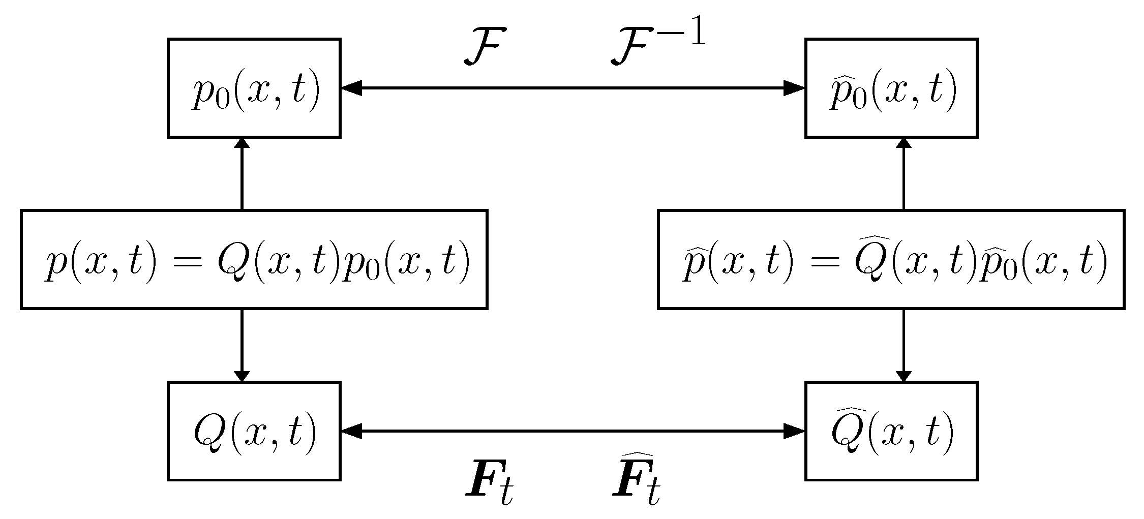
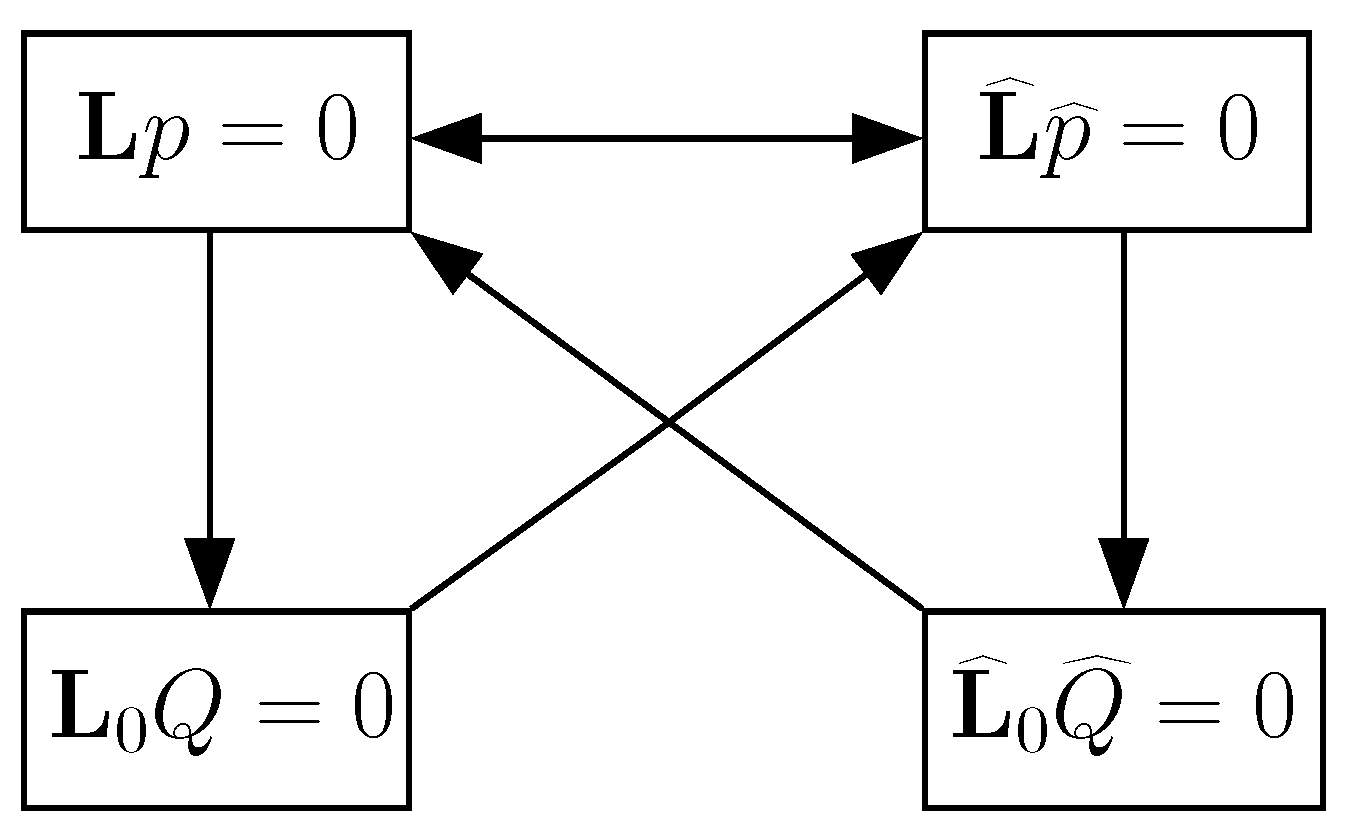
4.1. Mappings of Partial Differential Equations

Let us consider the following homogenous linear partial differential equation (PDE) with non-constant coefficients:

$$\frac{\partial p}{\partial t}-\sum _{j=0}^m\left(\sum _{r=0}^{n_j}{a}_{jr}\left(t\right)x^r\right)\frac{\partial j_p}{\partial x^j}=0,$$

(46)

where $a_{jr}\left(t\right)\in {\mathbb{M}}_t$; $j,m,n_j=0,1,$ .... The set ${\mathbb{M}}_t$ is defined as:

$${\mathbb{M}}_t=\left\{\frac{{\sum }_{k=0}^m{\alpha }_k{t}^k}{{\sum }_{l=0}^n{\beta }_l{t}^l}|m,n\in {\mathbb{Z}}_0;{\alpha }_k,{\beta }_l\in \mathbb{C};t\in \mathbb{R}\right\}.$$

(47)

The PDE (46) reads:

$$\mathbf{L}p=0,$$

(48)

where

$$\mathbf{L}:={\mathbf{D}}_t-\sum _{j=0}^m\left(\sum _{r=0}^{n_j}{a}_{jr}\left(t\right)x^r\right){\mathbf{D}}_x^j.$$

(49)

4.1.1. Mapping between $\mathbf{L}p$ and $\widehat{\mathbf{L}}\widehat{p}$

The Fourier operator $\mathcal{F}$ can be applied to (48) to transform (46) into a PDE with respect to $\widehat{p}=\mathcal{F}\left(p\right)$ using the relations (13):

$$\begin{array}{cc}\hfill \mathcal{F}\left(\mathbf{L}p\right)& =\mathcal{F}\left({\mathbf{D}}_t-\sum _{j=0}^m\left(\sum _{r=0}^{n_j}{a}_{jr}\left(t\right)x^r\right){\mathbf{D}}_x^j\right)\hfill \\ \hfill & ={\mathbf{D}}_t\widehat{p}-\sum _{j=0}^m\left(\left(\sum _{r=0}^{n_j}{a}_{jr}\left(t\right){\left(-i{\mathbf{D}}_x\right)}^r\right){\left(-ix\right)}^j\right)\widehat{p}.\hfill \end{array}$$

(50)

Applying the Weyl–Heisenberg identity ${\mathbf{D}}_{x}x=1+x{\mathbf{D}}_x$ [17] to (50) yields the partial differential equation:

$$\widehat{\mathbf{L}}\widehat{p}=0,$$

(51)

where

$$\widehat{\mathbf{L}}={\mathbf{D}}_t-\sum _{j=0}^{\widehat{m}}\left(\sum _{r=0}^{{\widehat{n}}_j}{\widehat{a}}_{jr}\left(t\right){\widehat{x}}^r\right){\mathbf{D}}_x^j.$$

(52)

The indices $\widehat{m},{\widehat{n}}_j$ and coefficients ${\widehat{a}}_{jr}\in {\mathbb{M}}_t$ are computed by applying the Weyl–Heisenberg identity and reordering the resulting expression.

4.1.2. Mapping between $\mathbf{L}p$ and ${\mathbf{L}}_{0}Q$

Operators ${\mathbf{R}}_x,{\mathbf{R}}_t$ (see Corollary 2) together with the expression $p=Q{p}_0$ can be used on the PDE (46) to obtain an equation with respect to the carrier polynomial Q:

$$\begin{array}{cc}\hfill \mathbf{L}p& ={\mathbf{D}}_{t}Q{p}_0-\sum _{j=0}^m\left(\sum _{r=0}^{n_j}{a}_{jr}\left(t\right)x^r\right){\mathbf{D}}_x^{j}Q{p}_0\hfill \\ \hfill & =\left(\left({\mathbf{D}}_t+\frac{1}{2}\left(\frac{x^2}{t^2}-\frac{1}{s}\right)\right)Q-\left(\sum _{j=0}^m\left(\sum _{r=0}^{n_j}{a}_{jr}\left(t\right)x^r\right){\mathbf{R}}_x^{j}Q\right)\right)p_0\hfill \\ \hfill & =\left(\left({\mathbf{D}}_t-\sum _{j=0}^{\overline{m}}\left(\sum _{r=0}^{{\overline{n}}_j}{b}_{jr}\left(t\right)x^r\right){\mathbf{D}}_x^j\right)Q\right)p_0.\hfill \end{array}$$

(53)

Canceling $p_0$ in (53) yields the following PDE with respect to Q:

$${\mathbf{L}}_{0}Q=0,$$

(54)

where

$${\mathbf{L}}_0={\mathbf{D}}_t-\sum _{j=0}^{\overline{m}}\left(\sum _{r=0}^{{\overline{n}}_j}{b}_{jr}\left(t\right)x^r\right){\mathbf{D}}_x^j,b_{jr}\in {\mathbb{M}}_t.$$

(55)

4.1.3. Mapping between ${\mathbf{L}}_{0}Q$ and $\widehat{\mathbf{L}}\widehat{p}$; $\widehat{\mathbf{L}}\widehat{p}$ and ${\widehat{\mathbf{L}}}_0\widehat{Q}$

Applying operators ${\mathsf{\Phi }}_x,{\mathsf{\Phi }}_t$ (see Corollary 3) to (54) yields PDE (51):

$$\begin{array}{cc}\hfill \mathcal{F}\left({\mathbf{L}}_{0}Q\right)p_0& =\mathcal{F}\left({\mathbf{D}}_{t}Q\right)p_0-\sum _{j=0}^{\overline{m}}\left(\sum _{r=0}^{{\overline{n}}_j}{b}_{jr}\left(t\right){\left(-i{\mathbf{D}}_x\right)}^j\right)\mathcal{F}\left({\mathbf{D}}_x^{j}Q\right)p_0\hfill \\ \hfill & ={\mathbf{D}}_t\widehat{p}+\frac{1}{2}\left(\frac{1}{t}+\frac{1}{2}{\mathbf{D}}_x^2\right)\widehat{p}-\sum _{j=0}^{\overline{m}}\left(\sum _{r=0}^{{\overline{n}}_j}{b}_{jr}\left(t\right){\left(-i{\mathbf{D}}_x\right)}^j\right){\mathsf{\Phi }}_x^j\widehat{p}\hfill \\ \hfill & =\left({\mathbf{D}}_t-\sum _{j=0}^{\widehat{m}}\left(\sum _{r=0}^{{\widehat{n}}_j}{\widehat{a}}_{jr}\left(t\right)x^r\right){\mathbf{D}}_x^j\right)\widehat{p}=\widehat{\mathbf{L}}\widehat{p}.\hfill \end{array}$$

(56)

Using analogous derivations with operators ${\widehat{\mathbf{R}}}_x,{\widehat{\mathbf{R}}}_t$, it can be shown that the Equation (51) yields a PDE with respect to $\widehat{Q}$:

$${\widehat{\mathbf{L}}}_0\widehat{Q}=0,$$

(57)

where

$${\widehat{\mathbf{L}}}_0={\mathbf{D}}_t-\sum _{j=0}^{\tilde{m}}\left(\sum _{r=0}^{{\tilde{n}}_j}{\widehat{b}}_{jr}\left(t\right)x^r\right){\mathbf{D}}_x^j,{\widehat{b}}_{jr}\in {\mathbb{M}}_t.$$

(58)

Other possible mappings are ${\mathbf{L}}_{0}Q$ to $\widehat{\mathbf{L}}\widehat{p}$ and ${\widehat{\mathbf{L}}}_0\widehat{Q}$ to $\mathbf{L}p$.

A diagram of the mappings between the discussed PDEs is given in Figure 2. Note that the mappings displayed in Figure 2 are sufficient to map any of the PDEs $\mathbf{L}p,\widehat{\mathbf{L}}\widehat{p},{\mathbf{L}}_{0}Q,{\widehat{\mathbf{L}}}_0\widehat{Q}$ to all of the remaining PDEs.

4.2. Formulation of Cauchy Initial Conditions

Cauchy problems on PDEs (48), (51), (54) and (57) can be formulated. Respective initial conditions read:

$$\begin{array}{cc}\hfill & p\left(x,t_0\right)=p_1\left(x\right);\hfill \end{array}$$

(59)

$$\begin{array}{cc}\hfill & \widehat{p}\left(x,t_0\right)={\widehat{p}}_1\left(x\right);\hfill \end{array}$$

(60)

$$\begin{array}{cc}\hfill & Q(x,t_0)=q_1\left(x\right);\hfill \end{array}$$

(61)

$$\begin{array}{cc}\hfill & \widehat{Q}\left(x,t_0\right)={\widehat{q}}_1\left(x\right).\hfill \end{array}$$

(62)

Note that initial conditions are consistent (in the sense that solutions which satisfy them do exist) only if $t_0>0$. However, a simple time-variable substitution $t=t-t_0,t_0\in \mathbb{R}$ allows to consider a wider range of initial conditions with respect to t.

As shown in the previous subsection, the four PDEs $\mathbf{L}p,\widehat{\mathbf{L}}\widehat{p},{\mathbf{L}}_{0}Q,{\widehat{\mathbf{L}}}_0\widehat{Q}$ can be related using the scheme displayed in Figure 2. Similarly, Cauchy initial conditions (59)–(62) satisfy the following relations:

$$\begin{array}{cc}\hfill & p_1\left(x\right)=q_1\left(x\right)p_0\left(x,t_0\right),{\widehat{p}}_1\left(x\right)={\widehat{q}}_1\left(x\right)\widehat{p}(x,t_0);\hfill \end{array}$$

(63)

$$\begin{array}{cc}\hfill & \mathcal{F}{p}_1\left(x\right)={\widehat{p}}_1\left(x\right),{\mathcal{F}}^{-1}{\widehat{p}}_1\left(x\right)=p_1\left(x\right);\hfill \end{array}$$

(64)

$$\begin{array}{cc}\hfill & q_1\left(x\right)=\widehat{q}\left({\widehat{\mathbf{F}}}_{t_0}\right)1,{\widehat{q}}_1\left(x\right)=q\left({\mathbf{F}}_{t_0}\right)1.\hfill \end{array}$$

(65)

Above equalities can also be used together with the mappings outlined in Section 4.1 to produce the mappings of Cauchy problems. Note that (63)–(65) are also consistency conditions that can be used to verify if given initial functions satisfy the same class of PDEs that can be mapped to each other (Equations (48), (51), (54) and (57)).

For the following computations it will assumed (without loss of generality) that $t_0=1$.

5. Several Examples

5.1. Solving Cauchy Problem Given the PDE

The mapping scheme constructed in this paper can be applied to obtain the solution of some PDEs by mapping them to PDEs which require polynomial solutions. Let us consider the following Cauchy problem with respect to $p(x,t)$:

$$\begin{array}{cc}\hfill & {\mathbf{D}}_{t}p=\frac{t^3}{2}{\mathbf{D}}_x^{4}p+t^{2}x{\mathbf{D}}_x^3+\left(\frac{1}{2}+3t^2+\frac{t{x}^2}{2}\right){\mathbf{D}}_x^{2}p+\frac{5tx}{2}{\mathbf{D}}_{x}p+\left(\frac{3t}{2}-\frac{1}{a-t}\right)p;t\ne a;\hfill \end{array}$$

(66)

$$\begin{array}{cc}\hfill & p(x,1)=p_1\left(x\right)=\left(a_0+a_{1}x+a_2{x}^2\right)\frac{1}{\sqrt{2\pi }}exp\left(-\frac{x^2}{2}\right),a_0,a_1,a_2\in \mathbb{R}.\hfill \end{array}$$

(67)

Thus,

$$\mathbf{L}:={\mathbf{D}}_t-\frac{t^3}{2}{\mathbf{D}}_x^4-t^{2}x{\mathbf{D}}_x^3-\left(\frac{1}{2}+3t^2+\frac{t{x}^2}{2}\right){\mathbf{D}}_x^2-\frac{5tx}{2}{\mathbf{D}}_x-\frac{3t}{2}+\frac{1}{a-t}.$$

(68)

Using the Fourier transform operator $\mathcal{F}$, the equation $\mathbf{L}p$ is transformed to $\widehat{\mathbf{L}}\widehat{p}$:

$$\widehat{\mathbf{L}}={\mathbf{D}}_t-\frac{t{x}^2}{2}{\mathbf{D}}_x^2+\left(\frac{tx}{2}-t^2{x}^3\right){\mathbf{D}}_x+\frac{1}{a-t}+\frac{x^2}{2}-\frac{t^3{x}^4}{2}.$$

(69)

Equation (69) results in the following Cauchy problem:

$$\begin{array}{cc}\hfill & {\mathbf{D}}_t\widehat{p}=\frac{t{x}^2}{2}{\mathbf{D}}_x^2\widehat{p}+\left(t^2{x}^3-\frac{tx}{2}\right){\mathbf{D}}_x\widehat{p}-\left(\frac{1}{a-t}+\frac{x^2}{2}-\frac{t^3{x}^4}{2}\right)\widehat{p};\hfill \end{array}$$

(70)

$$\begin{array}{cc}\hfill & \widehat{p}(x,1)={\widehat{p}}_1\left(x\right)=\left({\widehat{a}}_0+{\widehat{a}}_{1}x+{\widehat{a}}_{2}x\right)exp\left(-\frac{x^2}{2}\right),{\widehat{a}}_0,{\widehat{a}}_1,{\widehat{a}}_2\in \mathbb{C}.\hfill \end{array}$$

(71)

Using operators ${\widehat{R}}_x,{\widehat{R}}_t$, the Cauchy problem (70), Equation (71) is mapped to the following problem with respect to $\widehat{Q}$:

$$\begin{array}{cc}\hfill & {\mathbf{D}}_t\widehat{Q}=\frac{t{x}^2}{2}{\mathbf{D}}_x^2\widehat{Q}-\frac{tx}{2}{\mathbf{D}}_x\widehat{Q}-\frac{1}{a-t}\widehat{Q};\hfill \end{array}$$

(72)

$$\begin{array}{cc}\hfill & \widehat{Q}(x,1)={\widehat{q}}_1\left(x\right)={\widehat{a}}_0+{\widehat{a}}_{1}x+{\widehat{a}}_{2}x,{\widehat{a}}_0,{\widehat{a}}_1,{\widehat{a}}_2\in \mathbb{C}.\hfill \end{array}$$

(73)

Equation (72) can be solved for the solution that is polynomial in x and which satisfies the condition (73), yielding:

$$\widehat{Q}\left(x,t\right)=\frac{x^2}{2}\left(a-t\right),a\in \mathbb{R}.$$

(74)

The solution to (66) and (67) is constructed using the relations (25) and (26):

$$p(x,t)=\frac{(a-t)\left(t-x^2\right)}{2t^2\sqrt{2\pi t}}exp\left(-\frac{x^2}{2t}\right).$$

(75)

5.2. Mappings between PDEs

In this example, the mapping scheme described in Section 4.1 and pictured in Figure 2 is illustrated. Consider the following PDE with respect to $\widehat{Q}$:

$${\widehat{\mathbf{L}}}_0\widehat{Q}={\mathbf{D}}_t\widehat{Q}-\frac{k}{l}\frac{x}{t}{\mathbf{D}}_x\widehat{Q}=0.$$

(76)

With the following Cauchy initial condition:

$$\widehat{Q}(x,1)={\widehat{q}}_1\left(x\right)=\sum _{j=0}^m{\widehat{a}}_j{x}^{lj}.$$

(77)

The derivations discussed in Section 4.1 can be used to obtain PDEs (48), (51) and (54). For example:

$$\begin{array}{cc}\hfill {\mathcal{F}}^{-1}\left(\left({\widehat{\mathbf{L}}}_0\widehat{Q}\right){\widehat{p}}_0\right)& ={\mathcal{F}}^{-1}\left(\left({\mathbf{D}}_t\widehat{Q}\right){\widehat{p}}_0\right)-\frac{k}{lt}{\mathcal{F}}^{-1}\left(\left(x{\mathbf{D}}_x\widehat{Q}\right){\widehat{p}}_0\right)\hfill \\ \hfill & ={\widehat{\mathsf{\Phi }}}_t{\mathcal{F}}^{-1}\left(\widehat{Q}{\widehat{p}}_0\right)-\frac{ik}{ls}{\mathbf{D}}_x{\widehat{\mathsf{\Phi }}}_x{\mathcal{F}}^{-1}\left(\widehat{Q}{\widehat{p}}_0\right)\hfill \\ \hfill & ={\mathbf{D}}_{t}p+\frac{2k-l}{2l}{\mathbf{D}}_x^{2}p+\frac{k}{l}\frac{x}{t}{\mathbf{D}}_{x}p+\frac{k}{lt}p,\hfill \end{array}$$

(78)

thus,

$${\widehat{\mathbf{L}}}_0={\mathbf{D}}_t-\frac{k}{l}\frac{x}{t}{\mathbf{D}}_x\to \mathbf{L}={\mathbf{D}}_t+\frac{2k-l}{2l}{\mathbf{D}}_x^2+\frac{k}{l}\frac{x}{t}{\mathbf{D}}_x+\frac{k}{lt},$$

(79)

and the following Cauchy problem is equivalent to (76) and (77):

$$\begin{array}{cc}\hfill {\mathbf{D}}_{t}p& =\frac{l-2k}{2l}{\mathbf{D}}_x^{2}p-\frac{k}{l}\frac{x}{t}{\mathbf{D}}_{x}p-\frac{k}{lt}p;\hfill \\ \hfill p_1\left(x\right)& =\frac{1}{\sqrt{2\pi }}\left(\sum _{j=0}^m{\widehat{a}}_j\left({\widehat{\mathbf{F}}}_1^{lj}1\right)\right)exp\left(-\frac{x^2}{2}\right).\hfill \end{array}$$

(80)

In the same manner, it is possible to obtain Cauchy problems on $\widehat{p}$ and Q:

$$\begin{array}{cc}\hfill {\mathbf{D}}_t\widehat{p}& =\frac{k}{l}\frac{x}{t}{\mathbf{D}}_x\widehat{p}+\frac{2k-l}{2l}{x}^2\widehat{p};\hfill \\ \hfill {\widehat{p}}_1\left(x\right)& =\left(\sum _{j=0}^m{\widehat{a}}_j{x}^{lj}\right)exp\left(-\frac{x^2}{2}\right),\hfill \end{array}$$

(81)

and

$$\begin{array}{cc}\hfill {\mathbf{D}}_{t}Q& =\frac{l-2k}{2l}{\mathbf{D}}_x^{2}Q+\frac{k-l}{l}\frac{x}{t}{\mathbf{D}}_{x}Q;\hfill \\ \hfill q_1\left(x\right)& =\sum _{j=0}^m{\widehat{a}}_j\left({\widehat{\mathbf{F}}}_1^{lj}1\right).\hfill \end{array}$$

(82)

Note that constructing a solution to any of the four presented PDEs yields solutions to the remaining three via transformations provided in Section 4.1. It can be verified that the solutions to (76) have the following form [18]:

$$\widehat{Q}(x,t)=\sum _{j=0}^m{\widehat{a}}_j{\left(s^k{x}^l\right)}^j,{\widehat{a}}_j\in \mathbb{C}.$$

(83)

Which yields that the solutions to (80)–(82) read:

$$\begin{array}{cc}\hfill & p(x,t)=\frac{1}{\sqrt{2\pi t}}\left(\sum _{j=0}^m{\widehat{a}}_j\left({\widehat{\mathbf{F}}}_t^{lj}1\right)\right)exp\left(-\frac{x^2}{2t}\right);\hfill \end{array}$$

(84)

$$\begin{array}{cc}\hfill & \widehat{p}(x,t)=\sum _{j=0}^m{\widehat{a}}_j{\left(s^k{x}^l\right)}^{j}exp\left(-\frac{t{x}^2}{2}\right);\hfill \end{array}$$

(85)

$$\begin{array}{cc}\hfill & Q(x,t)=\sum _{j=0}^m{\widehat{a}}_j\left({\widehat{\mathbf{F}}}_t^{lj}1\right).\hfill \end{array}$$

(86)

These computations demonstrate the power of the method described in this paper. Equations such as (67) can be mapped to equations such as (72) that only require the determination of solutions that are polynomial in x to yield solutions to (67).

6. Concluding Remarks

A computational framework for the construction of analytic solutions to linear homogenous PDEs with variable coefficients is developed in this paper. A common approach for the construction of solutions to such PDEs consists of applying the wave variable transformation $\xi =t+\alpha x;\alpha \in \mathbb{R}$ to transform the PDE into an ODE. A closed-form solution to the ODE can be obtained via the generalized differential operator method [19]. It must be observed that the generalized differential operator method yields a closed-form solution only if the obtained ODE satisfies a set of special conditions [19].

The novelty of the proposed method is based on the introduction of F-operators. The strength of this method is based on the fact that the developed set of F-operators allows to transform the original PDE into a form for which direct integration of PDE becomes unnecessary.

The structure of the original PDE allows to split the solution into rational and exponential factors. Symbolic manipulation with the developed set of F-operators offers a convenient approach for the construction of the solution to the Cauchy problem. Several computational examples are used to demonstrate the efficacy of the proposed scheme.

However, it is clear that the proposed scheme is limited to a rather narrow class of diffusion type PDEs. The presented F-operator scheme can also be extended to accommodate a wider class of PDEs by modifying the F-operators to act on non-symmetrical generalized Gaussian solutions. This and other extensions of the F-operator calculus for a wider class of PDEs is a natural topic of future research.

References

1. Stein, D.B.; Guy, R.D.; Thomases, B. Immersed boundary smooth extension: A high-order method for solving PDE on arbitrary smooth domains using Fourier spectral methods. J. Comput. Phys. 2016, 304, 252–274. [Google Scholar] [CrossRef] [Green Version]
2. Yang, X.J.; Baleanu, D.; Srivastava, H.M. Local Fractional Integral Transforms and Their Applications; Academic Press: Cambridge, UK, 2016. [Google Scholar]
3. Bakhos, T.; Saibaba, A.K.; Kitanidis, P.K. A fast algorithm for parabolic PDE-based inverse problems based on Laplace transforms and flexible Krylov solvers. J. Comput. Phys. 2015, 299, 940–954. [Google Scholar] [CrossRef] [Green Version]
4. Sokhal, S.; Verma, S.R. A Fourier wavelet series solution of partial differential equation through the separation of variables method. Appl. Math. Comput. 2020, 388, 125480. [Google Scholar]
5. Pindza, E.; Owolabi, K.M. Fourier spectral method for higher order space fractional reaction–diffusion equations. Commun. Nonlinear Sci. Numer. Simul. 2016, 40, 112–128. [Google Scholar] [CrossRef] [Green Version]
6. Gong, Y.; Cai, J.; Wang, Y. Some new structure-preserving algorithms for general multi-symplectic formulations of Hamiltonian PDEs. J. Comput. Phys. 2014, 279, 80–102. [Google Scholar] [CrossRef]
7. Nazari-Golshan, A.; Nourazar, S.S.; Ghafoori-Fard, H.; Yildirim, A.; Campo, A. A modified homotopy perturbation method coupled with the Fourier transform for nonlinear and singular Lane-Emden equations. Appl. Math. Lett. 2013, 26, 1018–1025. [Google Scholar] [CrossRef]
8. Mahor, T.C.; Mishra, R.; Jain, R. Analytical solutions of linear fractional partial differential equations using fractional Fourier transform. J. Comput. Appl. Math. 2021, 385, 113202. [Google Scholar] [CrossRef]
9. Yang, Y.; Li, X.; Xiao, A. Fourier Pseudospectral Method for Fractional Stationary Schrödinger Equation. Appl. Numer. Math. 2021, 165, 137–151. [Google Scholar] [CrossRef]
10. Saridakis, Y.G.; Sifalakis, A.G.; Papadopoulou, E. Efficient numerical solution of the generalized Dirichlet-Neumann map for linear elliptic PDEs in regular polygon domains. J. Comput. Appl. Math. 2012, 236, 2515–2528. [Google Scholar] [CrossRef] [Green Version]
11. Vermeersch, B.; Mey, G.D. A shortcut to inverse Fourier transforms: Approximate reconstruction of transient heating curves from sparse frequency domain data. Int. J. Therm. Sci. 2010, 49, 1319–1332. [Google Scholar] [CrossRef]
12. Wang, J.; Dai, H.; Hui, Y. Conservative Fourier spectral scheme for higher order Klein-Gordon-Schrödinger equations. Appl. Numer. Math. 2020, 156, 446–466. [Google Scholar] [CrossRef]
13. Ji, B.; Zhang, L.; Sun, Q. A dissipative finite difference Fourier pseudo-spectral method for the symmetric regularized long wave equation with damping mechanism. Appl. Numer. Math. 2020, 154, 90–103. [Google Scholar] [CrossRef]
14. Huijskens, T.P.; Ruijter, M.J.; Oosterlee, C.W. Efficient numerical Fourier methods for coupled forward–backward SDEs. J. Comput. Appl. Math. 2016, 296, 593–612. [Google Scholar] [CrossRef]
15. Larsson, E.; Ahlander, K.; Hall, A. Multi-dimensional option pricing using radial basis functions and the generalized Fourier transform. J. Comput. Appl. Math. 2008, 222, 175–192. [Google Scholar] [CrossRef] [Green Version]
16. Temme, N. Special Functions: An Introduction to the Classical Functions of Mathematical Physics; Wiley: New York, NY, USA, 1996. [Google Scholar]
17. Feinsilver, P.; Schott, R. Algebraic Structures and Operator Calculus, Vol. I: Representations and Probability Theory; Kluwer Academic Publishers: Dordrecht, Germany, 1993. [Google Scholar]
18. Navickas, Z. Constructive solution of the Cauchy problem for a special class of partial differential equations with constant coefficients. Lith. Math. J. 1994, 34, 404–414. [Google Scholar] [CrossRef]
19. Navickas, Z.; Bikulciene, L.; Rahula, M.; Ragulskis, M. Algebraic operator method for the construction of solitary solutions to nonlinear differential equations. Commun. Nonlinear Sci. Numer. Simul. 2013, 18, 1374–1389. [Google Scholar] [CrossRef]
Figure 1. The relationship between the generalized Gaussian function p, the carrier polynomial Q and their respective images.
Mathematics 09 00918 g001
Figure 2. Mappings between PDEs with respect to the generalized Gaussian function p, their carrier polynomials Q and their respective images.
Mathematics 09 00918 g002
Publisher’s Note: MDPI stays neutral with regard to jurisdictional claims in published maps and institutional affiliations.