An Analytical EM Algorithm for Sub-Gaussian Vectors

Abstract

The area in which a multivariate $\alpha$-stable distribution could be applied is vast; however, a lack of parameter estimation methods and theoretical limitations diminish its potential. Traditionally, the maximum likelihood estimation of parameters has been considered using a representation of the multivariate stable vector through a multivariate normal vector and an $\alpha$-stable subordinator. This paper introduces an analytical expectation maximization (EM) algorithm for the estimation of parameters of symmetric multivariate $\alpha$-stable random variables. Our numerical results show that the convergence of the proposed algorithm is much faster than that of existing algorithms. Moreover, the likelihood ratio (goodness-of-fit) test for a multivariate $\alpha$-stable distribution was implemented. Empirical examples with simulated and real world (stocks, AIS and cryptocurrencies) data showed that the likelihood ratio test can be useful for assessing goodness-of-fit.

1. Introduction

Several empirical studies confirm that the real financial market data are often skewed and heavy-tailed (e.g., [1,2,3]). Therefore, a Gaussian distribution rarely fits the data—for example, stock returns or risk factors are badly fit by this law [4,5]. Note that the $\alpha$-stable distribution offers a reasonable improvement, if not the best choice, among the alternative distributions that have been proposed in the literature (e.g., [6,7]). Thus, normal distributions are usually substituted by more general stable distributions that allow us to model both the effects of leptokurtosis and asymmetry in the data.

In the one-dimensional case, the distribution of the random $\alpha$-stable variable is characterized by four parameters: the tail (stability) parameter $\alpha \in \left(0;2\right]$, skewness $\beta \in \left[-1;1\right]$, scale $\sigma >0$ and position $\mu \in {\Re }^1$. The stability parameter $\alpha$ is the most important, because it describes the behavior of the tails [2]. Moreover, when $\alpha \to 2$, the distribution of the random variable is equivalent to a normal distribution and $\beta \to 0$ (normal tail behavior). If $\alpha \to 0$, then the distribution becomes degenerate (extremely heavy tails). For example, Fielitz and Smith [8] showed that a symmetric univariate $\alpha$-stable distribution appears to be appropriate when stock prices are modeled. Rachev and Mittnik [2] estimated the parameters of autoregressive-moving-average models with asymmetric stable Paretian distributions. Kabasinskas et al. [9] proposed a mixed-stable model to model the intra-daily data from German DAX component stock returns. Furthermore, the parameters of the stable distribution collectively and the skewed t-distribution, calculated on the basis of stock data, were applied to predict the direction of the change in future Accounting and Governance Risk rating [10]. Ogata [11] revealed that cryptocurrencies are a special class of assets. During various clustering procedures, parameters of $\alpha$-stable distribution (together with other) were used as the main features.

One of the most recent applications of $\alpha$-stable and truncated $\alpha$-stable distributions in pension fund selection was published by Kopa [12]. They used first-, second- and third-order stochastic dominance rules to select the best pension fund from second pillar in Lithuania on the basis of the risk profile of the participant.

Furthermore, the multivariate $\alpha$-stable symmetric vector with the stability parameter $\alpha$ is expressed through a normally distributed random vector whose variance is distributed by an $\frac{\alpha }{2}$-stable distribution [13,14,15,16]

$$\mathbf{X}=\mathbf{\mu }+\sqrt{s_1}·{\mathbf{s}}_2,$$

(1)

where $s_1$ is a subordinator with the stability parameter $\frac{\alpha }{2}<1$; ${\mathbf{s}}_2$ is a random vector, distributed by the d-variate normal law $N\left(0,\mathbf{\Omega }\right)$; and $\mathbf{\mu }$ is a random vector of the means. The random $\alpha$-stable variable with $\frac{\alpha }{2}<1$ and $\beta =1$ is called a subordinator. In general, a subordinator is a one-dimensional non-decreasing Lévy process [17]. The estimation of parameters of multivariate $\alpha$-stable distributions has been a possibility for long time [18,19,20,21,22,23]; however, researchers emphasize that methods of the estimation of parameters still have weaknesses. For example, the authors of [20] gave an example of an application of the elliptical sub-Gaussian distribution to DAX 30 and reported how to deal with issues when the $\alpha$ values of underlying assets are different and data are asymmetric; however, they could not incorporate time dependencies. Daul [24] explained how to deal with large portfolios when assets have very different marginal distributions ($\alpha$s are very different). Furthermore, Nolan [25] gave an example of how to use it for Dow Jones 30 portfolios and introduced how to solve tail and serial dependency issues. Moreover, Kouaissah [26] showed how to use parametric multivariate stochastic dominance in the case of a sub-Gaussian distribution, even with different tail parameters. Such results are crucial in portfolio selection and management problems. However, practical applications of the multivariate stable law are limited by the fact that its distribution and density functions are not expressed through elementary functions. That said, Ravishanker’s group and Rezakhah’s group [15,27] reported the estimation of parameters of sub-Gaussian vectors by stochastic EM algorithms. The MCMC approach for the maximum likelihood estimation of model parameters ($\mathbf{\mu },\mathbf{\Omega },\alpha$) was considered by Ravishanker [15]. However, the accuracy of stochastic methods (e.g., [27]) is highly dependent on internal sample size, the error of stochastic integration and convergence criteria.

The analytical EM parameter estimation approach is considered in this paper. Since the probability density function (see the next section) of a random symmetric multivariate $\alpha$-stable vector might be expressed through bivariate integrals, it may be calculated using Gaussian and Gauss–Laguerre quadratures instead of using stochastic integration. This approach increases accuracy, simplifies the calculation of likelihood functions and increases computational efficiency compared to regular MLE methods and stochastic EM algorithms.

Now, let us discuss goodness-of-fit tests that were used in similar studies. The well known Kolmogorov–Smirnov test [28,29] is sensitive to differences in the position and shape of the sample distribution. It is extremely difficult to implement the proposed methods, as they require a transformation whose derivation is analytically intractable for most multivariate distributions. Another famous goodness-of-fit test is the Anderson–Darling test [30], which is used to estimate statistical differences between observed values and theoretical univariate distributions. However, there has been no multivariate case for this test created yet. Goodness-of-fit tests for univariate, symmetric, $\alpha$-stable distributions were considered by Matsui and Takemura [31]. Their methodology requires complicated numerical integration in order to preform goodness-of-fit tests for symmetric stable distributions. A completely different approach based on the empirical characteristic function tests for the multivariate stable distributions was considered by Meintanis [32]. However, they used weighted $L_2$-type statistics that are difficult to compute. In [33], specific goodness-of-fit test for multivariate normal distributions are proposed. The authors claimed that their test is overall the most powerful and is effective against skewed, long-tailed and short-tailed symmetric alternatives. Moreover, they claimed that this test can be used for testing fitness for an assumed p-variate non-normal distribution. However, the major weakness of the test is related to the proposed test statistics. McAssey [34] introduced a technique of a goodness-of-fit test for general multivariate distributions based on multivariate normal, uniform, Student’s t and beta distributions. This method is simple to implement, involves a reasonable computational burden and does not require analytically intractable derivations. It has sufficient power to detect a poor fit in most situations. However, the authors did not provide evidence that such a technique could be used for a multuvariate $\alpha$-stable distribution.

As an alternative to the mentioned goodness-of-fit tests, in this paper, we suggest a likelihood ratio test (developed in [35]). This test has never been used in the scientific literature for the goodness-of-fit of multivariate $\alpha$-stable distributions. However, this likelihood ratio test is computationally fast and does not require specific knowledge. The only two things that must be known are how to generate random variables and how to compute a likelihood function.

The paper is structured as follows: the likelihood function and the maximum likelihood method are described in Section 2. The EM algorithm is considered and applications of the Gaussian and Gauss–Laguerre quadrature formulas for bivariate integration are discussed in Section 2.3. The likelihood ratio test for distribution fitting with the estimated parameters is given in Section 2.4. In Section 3, we provide evidence of the convergence of the EM algorithm and real world examples with stock data, biomedical data and cryptocurrency data. Finally, we provide empirical recommendations in Section 3.5 and discuss our findings in Section 4.

2. Materials and Methods

In this section, we introduce maximum likelihood estimates of a multivariate $\alpha$-stable distribution, the proposed expectation maximization (EM) algorithm, quadrature formulas and the likelihood ratio test. The experimental design is also presented at the end of this section.

2.1. Maximum Likelihood Estimation

Maximum likelihood estimates (MLE) of parameters of any model are obtained by maximizing the likelihood function, calculated for a sample consisting of independent vectors [5,15,36,37]. Let us consider the probability density of a random vector created according to Equation (1). Indeed, the density of the d-dimensional normal vector $N\left(\mathbf{\mu },s·\mathbf{\Omega }\right)$ is as follows:

$$N(\left.x\right|\mu ,s,\mathbf{\Omega })=\frac{s^{-\frac{d}{2}}}{{\left(2\pi \right)}^{\frac{d}{2}}·{\left|\mathbf{\Omega }\right|}^{\frac{1}{2}}}·exp\left[-\frac{{\left(x-\mathbf{\mu }\right)}^T·{\mathbf{\Omega }}^{-1}·\left(x-\mathbf{\mu }\right)}{2·s}\right],$$

where $\left|\mathbf{\Omega }\right|>0$, $d⩾1$.

Now, let us write down the probability density of an $\alpha$-stable subordinator [2,38]:

$$S\left(s\left|\alpha \right.\right)=\frac{\alpha ·s^{\frac{2}{\alpha -2}}}{2·\left|2-\alpha \right|}\underset{-1}{\overset{1}{\int }}{U}_{{}_{\alpha }}^{\frac{\alpha }{2-\alpha }}\left(y\right)·exp\left[-{\left(\frac{U_{\alpha }\left(y\right)}{s}\right)}^{\frac{\alpha }{2-\alpha }}\right]dy,$$

where $s⩾0$, $-1⩽y⩽1$, $0<\alpha ⩽2$ and

$$U_{\alpha }\left(y\right)=\frac{sin\left(\frac{\pi }{4}·\alpha ·\left(y+1\right)\right)·cos{\left(\frac{\pi }{4}·\left(\alpha -\left(2-\alpha \right)·y\right)\right)}^{\frac{2-\alpha }{\alpha }}}{cos{\left(\pi ·\frac{y}{2}\right)}^{\frac{2}{\alpha }}·cos{\left(\frac{\pi ·\alpha }{4}\right)}^{\frac{2}{\alpha }}}.$$

Thus, the probability density of a symmetric multivariate $\alpha$-stable random vector with given parameters $\mathbf{\mu },\mathbf{\Omega },\alpha$ is expressed as a bivariate integral:

$$\begin{array}{c}f\left(\left.x\right|\mathbf{\mu },\mathbf{\Omega },\alpha \right)=\frac{\left(\frac{\alpha }{2-\alpha }\right)}{2·{\left(2\pi \right)}^{\frac{d}{2}}·{\left|\mathbf{\Omega }\right|}^{\frac{1}{2}}}\times \hfill \\ \times \underset{0}{\overset{\infty }{\int }}\underset{-1}{\overset{1}{\int }}exp\left[-\frac{1}{2}{\left(x-\mathbf{\mu }\right)}^T\frac{{\mathbf{\Omega }}^{-1}}{s}\left(x-\mathbf{\mu }\right)-{\left(\frac{U_{\alpha }\left(y\right)}{s}\right)}^{\frac{\alpha }{2-\alpha }}\right]\frac{U_{{}_{\alpha }}^{\frac{\alpha }{2-\alpha }}\left(y\right)}{s^{\frac{2}{2-\alpha }+\frac{d}{2}}}dyds.\hfill \end{array}$$

(2)

However, it is very difficult to use this function in practice, even in a univariate case.

Let us consider the sample $\mathit{X}=\left(X^1,X^2,\dots ,X^K\right)$ consisting of independent d-variate $\alpha$-stable vectors. The likelihood function by virtue of (2) is

$$\begin{array}{c}\tilde{L}\left(\mathbf{X},\mathbf{\mu },\mathbf{\Omega },\alpha \right)={\displaystyle \prod _{i=1}^K}f\left(\left.X^i\right|\mathbf{\mu },\mathbf{\Omega },\alpha \right)=\frac{{\left(\frac{\alpha }{2-\alpha }\right)}^K}{2^K·{\left(2\pi \right)}^{\frac{K·d}{2}}·{\left|\mathbf{\Omega }\right|}^{\frac{K}{2}}}\times \hfill \\ \times {\displaystyle \prod _{i=1}^K}\underset{0}{\overset{\infty }{\int }}\underset{-1}{\overset{1}{\int }}exp\left[-\frac{1}{2}{\left(X^i-\mathbf{\mu }\right)}^T\frac{{\mathbf{\Omega }}^{-1}}{s}\left(X^i-\mathbf{\mu }\right)-s^{\frac{\alpha }{\alpha -2}}·U_{{}_{\alpha }}^{\frac{\alpha }{2-\alpha }}\left(y\right)\right]·\frac{U_{{}_{\alpha }}^{\frac{\alpha }{2-\alpha }}\left(y\right)}{s^{\frac{d}{2}+\frac{2}{2-\alpha }}}dyds.\hfill \end{array}$$

The maximum likelihood estimates can be obtained by maximizing the latter function with respect to $\mathbf{\mu },\mathbf{\Omega }$ and $\alpha$. Note that very small or very large values of it can occur during numerical calculations. Therefore, from a computational point of view, it is reasonable to use the log-likelihood function (LLF):

$$\begin{array}{c}L\left(\mathbf{X},\mathbf{\mu },\mathbf{\Omega },\alpha \right)=-ln\left(\tilde{L}\left(\mathbf{X},\mathbf{\mu },\mathbf{\Omega },\alpha \right)\right)=-{\displaystyle \sum _{i=1}^K}ln\left(f\left(\left.X^i\right|\mathbf{\mu },\mathbf{\Omega },\alpha \right)\right)=\hfill \\ =-{\displaystyle \sum _{i=1}^K}ln\left(\underset{0}{\overset{\infty }{\int }}exp\left\{-z\right\}{\displaystyle \underset{-1}{\overset{1}{\int }}}B\left(X^i,y,z,\mathbf{\mu },\mathbf{\Omega },\alpha \right)dydz\right),\hfill \end{array}$$

(3)

where $B(·)$ is denoted as

$$B\left(x,y,z,\mathbf{\mu },\mathbf{\Omega },\alpha \right)=\frac{1}{2·{\left(2\pi \right)}^{\frac{d}{2}}·{\left|\mathbf{\Omega }\right|}^{\frac{1}{2}}·U_{{}_{\alpha }}^{\frac{d}{2}}\left(y\right)}·z^{\frac{d·\left(2-\alpha \right)}{2·\alpha }}·exp\left\{-\frac{{\left(x-\mathbf{\mu }\right)}^T{\mathbf{\Omega }}^{-1}\left(x-\mathbf{\mu }\right)}{2·U_{\alpha }\left(y\right)}·z^{\frac{2-\alpha }{\alpha }}\right\},$$

where the substitution of integration variable is $z=s^{\frac{\alpha }{\alpha -2}}·U_{{}_{\alpha }}^{\frac{\alpha }{2-\alpha }}\left(y\right)$. The latter substitution is useful in Gauss–Laguerre quadrature for numerical integration (see Section 2.3).

Hence, the estimates of parameters $\widehat{\mathbf{\mu }},\widehat{\mathbf{\Omega }}$ and $\widehat{\alpha }$ are obtained by minimizing the LLF

$$L\left(\mathbf{X},\widehat{\mathbf{\mu }},\widehat{\mathbf{\Omega }},\widehat{\alpha }\right)=\underset{\mathbf{\mu },\mathbf{\Omega },\alpha }{min}L\left(\mathbf{X},\mathbf{\mu },\mathbf{\Omega },\alpha \right).$$

(4)

This optimization problem may be solved in many ways; however, it is very time consuming and inefficient. In the next section, we introduce the expectation maximization approach in MLE estimation.

2.2. The Expectation Maximization Algorithm

Let us consider a two-step recurrent procedure, in which the parameters $\mathbf{\mu }$ and $\mathbf{\Omega }$ of the multivariate $\alpha$-stable distribution are estimated at each iteration by the expectation maximization (EM) algorithm, and then $\alpha$ is estimated by solving the corresponding univariate optimization problem.

Since LLF is an analytical function, its partial derivatives with respect to $\mathbf{\mu }$ and $\mathbf{\Omega }$ can be found. Hence, if $\alpha$ is fixed, then the Maximal Likelihood estimates of the parameters $\mathbf{\mu }$ and $\mathbf{\Omega }$ can be found by setting partial derivatives of (3) to zero and solving the corresponding system of nonlinear equations:

$$\left\{\begin{array}{c}\frac{\partial L\left(\mathbf{X},\mathbf{\mu },\mathbf{\Omega },\alpha \right)}{\partial \mathbf{\mu }}=-{\displaystyle \sum _{i=1}^K}\frac{\partial f\left(\left.X^i\right|\mathbf{\mu },\mathbf{\Omega },\alpha \right)}{\partial \mathbf{\mu }}·\frac{1}{f\left(\left.X^i\right|\mathbf{\mu },\mathbf{\Omega },\alpha \right)}=0,\hfill \\ \frac{\partial L\left(\mathbf{X},\mathbf{\mu },\mathbf{\Omega },\alpha \right)}{\partial \mathbf{\Omega }}=-{\displaystyle \sum _{i=1}^K}\frac{\partial f\left(\left.X^i\right|\mathbf{\mu },\mathbf{\Omega },\alpha \right)}{\partial \mathbf{\Omega }}·\frac{1}{f\left(\left.X^i\right|\mathbf{\mu },\mathbf{\Omega },\alpha \right)}=0.\hfill \end{array}\right.$$

Using the rules of differentiation with respect to vector or matrix [39], one can write the derivatives

$$\begin{array}{c}\frac{\partial B\left(x,y,z,\mathbf{\mu },\mathbf{\Omega },\alpha \right)}{\partial \mathbf{\mu }}=-\frac{1}{2·{\left(2\pi \right)}^{\frac{d}{2}}·{\left|\mathbf{\Omega }\right|}^{\frac{1}{2}}·U_{{}_{\alpha }}^{\frac{d}{2}+1}\left(y\right)}·z^{\frac{\left(d+2\right)·\left(2-\alpha \right)}{2·\alpha }}·{\mathbf{\Omega }}^{-1}\left(x-\mathbf{\mu }\right)\times \hfill \\ \times exp\left\{-\frac{{\left(x-\mathbf{\mu }\right)}^T{\mathbf{\Omega }}^{-1}\left(x-\mathbf{\mu }\right)}{2·U_{\alpha }\left(y\right)}·z^{\frac{2-\alpha }{\alpha }}\right\}=\frac{{\mathbf{\Omega }}^{-1}\left(x-\mathbf{\mu }\right)}{U_{\alpha }\left(y\right)}·z^{\frac{2-\alpha }{\alpha }}·B\left(x,y,z,\mathbf{\mu },\mathbf{\Omega },\alpha \right),\hfill \\ \frac{\partial B\left(x,y,z,\mathbf{\mu },\mathbf{\Omega },\alpha \right)}{\partial \mathbf{\Omega }}=\frac{1}{2·{\left(2\pi \right)}^{\frac{d}{2}}·{\left|\mathbf{\Omega }\right|}^{\frac{1}{2}}·U_{{}_{\alpha }}^{\frac{d}{2}+1}\left(y\right)}·z^{\frac{\left(d+2\right)·\left(2-\alpha \right)}{2·\alpha }}·\left(-{\mathbf{\Omega }}^{-1}+{\mathbf{\Omega }}^{-1}·(x-\mathbf{\mu })·{(x-\mathbf{\mu })}^T·{\mathbf{\Omega }}^{-1}\right)\times \hfill \\ \times exp\left\{-\frac{{\left(x-\mathbf{\mu }\right)}^T{\mathbf{\Omega }}^{-1}\left(x-\mathbf{\mu }\right)}{2·U_{\alpha }\left(y\right)}·z^{\frac{2-\alpha }{\alpha }}\right\}=\hfill \\ =\left(-{\mathbf{\Omega }}^{-1}+\frac{{\mathbf{\Omega }}^{-1}·(x-\mathbf{\mu })·{(x-\mathbf{\mu })}^T·{\mathbf{\Omega }}^{-1}}{U_{\alpha }\left(y\right)}·z^{\frac{2-\alpha }{\alpha }}\right)·B\left(x,y,z,\mathbf{\mu },\mathbf{\Omega },\alpha \right).\hfill \end{array}$$

Let us denote a few important functions $g_i$, $f_i$, $h(·)$ and $w(·)$

$$g_i=g\left(\left.X^i\right|\mathbf{\mu },\mathbf{\Omega },\alpha \right)=\underset{0}{\overset{\infty }{\int }}\left(\underset{-1}{\overset{1}{\int }}\frac{B\left(X^i,y,z,\mathbf{\mu },\mathbf{\Omega },\alpha \right)}{U_{\alpha }\left(y\right)}dy\right)z^{\frac{2-\alpha }{\alpha }}exp\left\{-z\right\}dz,$$

(5)

$$f_i=f\left(\left.X^i\right|\mathbf{\mu },\mathbf{\Omega },\alpha \right)=\underset{0}{\overset{\infty }{\int }}\left(\underset{-1}{\overset{1}{\int }}B\left(X^i,y,z,\mathbf{\mu },\mathbf{\Omega },\alpha \right)dy\right)exp\left\{-z\right\}dz,1⩽i⩽K,$$

(6)

$$h\left(\mathbf{X},\mathbf{\mu },\mathbf{\Omega },\alpha \right)=\frac{{\displaystyle \sum _{i=1}^K}\frac{X^i·g_i}{f_i}}{{\displaystyle \sum _{i=1}^K}\frac{g_i}{f_i}},$$

$$w\left(\mathbf{X},\mathbf{\mu },\mathbf{\Omega },\alpha \right)=\sum _{i=1}^K\frac{\left(X^i-\widehat{\mathbf{\mu }}\right){\left(X^i-\widehat{\mathbf{\mu }}\right)}^T{g}_i}{f_i}.$$

Using the notation from above, the derivatives of LLF can be rewritten in the following way:

$$\frac{\partial L}{\partial \mathbf{\mu }}=\left(h\left(\mathbf{X},\mathbf{\mu },\mathbf{\Omega },\alpha \right)-\mathbf{\mu }\right)·\sum _{i=1}^K\frac{g_i}{f_i},$$

$$\frac{\partial L}{\partial \mathbf{\Omega }}=-K·{\mathbf{\Omega }}^{-1}+{\mathbf{\Omega }}^{-1}·w\left(\mathbf{X},\mathbf{\mu },\mathbf{\Omega },\alpha \right)·{\mathbf{\Omega }}^{-1}.$$

By setting the later derivatives to zero, one can write down the fixed point equations for MLE:

$$\widehat{\mathbf{\mu }}=h\left(\mathbf{X},\widehat{\mathbf{\mu }},\widehat{\mathbf{\Omega }},\widehat{\alpha }\right)$$

and

$$\widehat{\mathbf{\Omega }}=\frac{1}{K}w\left(\mathbf{X},\widehat{\mathbf{\mu }},\widehat{\mathbf{\Omega }},\widehat{\alpha }\right).$$

Assume the initial values ${\mathbf{\mu }}^0$, ${\mathbf{\Omega }}^0$ and ${\alpha }^0$ are chosen. Then, k iterations of the EM algorithm can be generated and estimates ${\mathbf{\mu }}^k$, ${\mathbf{\Omega }}^k$ and ${\alpha }^k$ at each iteration can be computed [40,41]. Following the two-step approach, estimates of the mean and covariance matrix are calculated for a particular tail parameter ${\alpha }^k$:

$${\mathbf{\mu }}^{k+1}=h\left(\mathbf{X},{\mathbf{\mu }}^k,{\mathbf{\Omega }}^k,{\alpha }^k\right)$$

(7)

$${\mathbf{\Omega }}^{k+1}=w\left(\mathbf{X},{\mathbf{\mu }}^k,{\mathbf{\Omega }}^k,{\alpha }^k\right)$$

(8)

Thus, an estimate of a stability parameter $\alpha$ at the $(k+1)$th step is obtained by solving the univariate LLF minimization problem:

$${\alpha }^{k+1}=arg\underset{0<\alpha ⩽2}{min}L\left(\mathbf{X},{\mathbf{\mu }}^{k+1},{\mathbf{\Omega }}^{k+1},\alpha \right)$$

(9)

Our empirical studies show that the LLF for fixed parameters $\mathbf{\mu }$ and $\mathbf{\Omega }$ is unimodal with respect to the stability parameter $\alpha$ (for examples, see Results Section). Hence, in the current study, the golden section search method is applied to the minimization of (9).

The sample mean vector and sample covariance matrix can be selected correspondingly as initial values of $\mathbf{\mu }$ and $\mathbf{\Omega }$:

$${\mathbf{\mu }}^0=\frac{1}{K}\sum _{i=1}^K{X}^i$$

(10)

and

$${\mathbf{\Omega }}^0=\frac{1}{K}\sum _{i=1}^K\left(X^i-{\mathbf{\mu }}^0\right)·{\left(X^i-{\mathbf{\mu }}^0\right)}^T.$$

(11)

Hence, the initial value of the stability parameter can be taken as ${\alpha }^0=1.5$. Many literature sources support this assumption, since, usually, for financial datasets, the tail parameter is from interval $\left(1;2\right)$ (e.g., see [4]). Mainly, the value is greater than 1.5 for assets from developed financial markets, and it is smaller for cryptocurrencies and emerging markets.

2.3. Gauss and Gauss–Laguerre Quadratures

Integrals in the expressions of the LLF (3), and corresponding estimates and minimization problems (4) or (7)–(9), can be computed by subroutines of mathematical programming systems such as MathCad and Maple, or using open source code, e.g., R or Python. Computational experiments with the $\alpha$-stable models of several variables have shown that solving (4) or (7)–(9) using MathCad (on PC Intel(R) Core(TM) i5, CPU 2.40 GHz, RAM 4.00 GB, OS 64-bit) usually requires many hours of processing time (see [16], Section 6.1). Since such computational time can be unacceptable in many applications, it is wise to implement the quadrature formulas for integration. Let us consider the Gaussian and Gauss–Laguerre quadrature formulas for the calculation of integrals in LLF and related expressions [41,42,43,44].

Thus, to calculate the integrals in Equations (3), (5) and (6) with respect to y, Gaussian quadrature formulas are used:

$$\underset{-1}{\overset{1}{\int }}f\left(y\right)dy\cong \sum _{i=1}^m{\vartheta }_{i}f\left(y_i\right),$$

(12)

where $f\left(y_i\right)$ is an integrated function, ${\vartheta }_i$ and $y_i$ are the Gaussian quadrature weights and nodes over [−1, 1] and m is the number of nodes. The positions $y_i$ (termed nodes) and weighting coefficients ${\vartheta }_i$ (termed weights) are chosen such that the integral is evaluated exactly by the quadrature (12), for some class of functions f (usually polynomials of a given degree). The Gaussian quadrature nodes $y_i$ are roots of polynomials $P_m\left(y\right)$ and can be computed by any root-finding algorithm [44].

To calculate the integrals in (3), (5) and (6) with respect to z, the Gauss–Laguerre quadrature formulas are applicable.

$$\underset{0}{\overset{\infty }{\int }}{z}^{\gamma }{e}^{-z}f\left(z\right)dz\cong \sum _{i=1}^n{\kappa }_{i}f\left(z_i\right),$$

(13)

where $f\left(z_i\right)$ is an integrated function, ${\kappa }_i$ and $z_i$ are the Gaussian–Laguerre quadrature weights and nodes (the ith zeros of Laguerre polynomials $L_n^{\gamma }\left(z\right)$) over [0, ∞] and n is the number of nodes. Note that the appropriate choice of parameter $\gamma$ with respect to the dimensionality of the problem and the initial value of the tail parameter $\alpha$ can improve calculation time. In this study, we set $\gamma =0$.

Computational experiments showed that it is enough to take Gauss–Laguerre quadrature with 20 nodes and 70 nodes for Gaussian quadrature to guaranty admissible accuracy of the corresponding calculations. Tables of the nodes and weights for Gaussian and Gaussian–Laguerre quadratures can be found in [42].

2.4. A Likelihood Ratio Test for Multivariate, $\alpha$-Stable Distribution

There are any different and reliable goodness-of-fit tests that could be used to test whether data fit a univariate distribution well. However, this cannot be said about the multivariate case. Among other multivariate (Kolmogorov–Smirnov, based on the characteristic function, based on specific test statistics, based on a beta function, etc.) methods, the most simple and straightforward is the likelihood ratio test [35].

The likelihood ratio test [45] can be applied to asses the quality of the MLE estimation of the multivariate $\alpha$-stable model too. The set of parameters ($\widehat{\mathbf{\mu }},\widehat{\mathbf{\Omega }},\widehat{\alpha }$) of the model is assumed to be known when considering the likelihood ratio test for distribution fitting to some data sample $\mathit{X}$.

The method works as follows. At the beginning, N multivariate random vectors $\mathit{Y}$ with $\alpha$-stable parameter estimates ($\widehat{\mathbf{\mu }},\widehat{\mathbf{\Omega }},\widehat{\alpha }$) are simulated. Then, the empirical distribution function $F_{\mathit{Y}}^{\left(n\right)}(x,\widehat{\mathbf{\mu }},\widehat{\mathbf{\Omega }},\widehat{\alpha })$ from the values of LLF (from generated random vectors $\mathit{Y}$) is constructed. Secondly, the likelihood $LLF{}_X$ value of initial data sample $\mathit{X}$ is compared with this empirical distribution $F_{\mathit{Y}}^{\left(n\right)}(x,·)$ [45]. If the empirical probability $F_{\mathit{Y}}^{\left(n\right)}(LL{F}_X,\widehat{\mathbf{\mu }},\widehat{\mathbf{\Omega }},\widehat{\alpha })$ of the latter value is within the interval $\left(\frac{p}{2},1-\frac{p}{2}\right)$, with p indicating significance, then there is no reason to reject the fitness hypothesis. More precisely, in our case, there is no reason to reject the fitness of underlying samples with the multivariate $\alpha$-stable law with estimated parameters ($\widehat{\mathbf{\mu }},\widehat{\mathbf{\Omega }},\widehat{\alpha }$) (for examples, see Section 3.2, Section 3.3 and Section 3.4).

2.5. Experimental Design

Now, let us describe the experiment. First, we generated multivariate $\alpha$-stable random variables $\mathit{X}$ using techniques described in [15]. Secondly, we estimated a set of parameters ($\widehat{\mathbf{\mu }},\widehat{\mathbf{\Omega }},\widehat{\alpha }$) of sample $\mathbf{X}$ using different algorithms (direct minimization of (3) and analytical EM algorithm). We assumed that direct minimization of (3) gives “true” estimates of parameters $\widehat{\mathbf{\mu }}$, $\widehat{\mathbf{\Omega }}$ and $\widehat{\alpha }$. To assess the quality of the EM algorithm, we simulated more (M) data samples with the same parameters $\widehat{\mathbf{\mu }},\widehat{\mathbf{\Omega }},\widehat{\alpha }$. From each iteration, we collected information and checked the convergence of the EM algorithm. If the LLF value and parameter estimates converged (with precision ${10}^{-8}$) to a value obtained by direct MLE, then we could say that the proposed algorithm converged and was reliable. Later, we proceeded with a goodness-of-fit test (likelihood ratio test). Finally, we give three real word examples: the stock market, biomedicine and cryptocurrency.

3. Results

The estimation of MLE $\alpha$-stable parameters by the EM algorithm is an iterative process that requires one to choose initial values, (10) and (11), and perform a certain number of iterations—(7)–(9)—while the values in adjacent steps differ insignificantly. To test the behavior of the designed algorithm, the experiments were performed with simulated and real world data. The integrals were calculated using the Gaussian (12) and the Gauss–Laguerre (13) quadratures.

3.1. Test Data Modeling

To test the convergence of the proposed analytical EM algorithm, the following experiment was conducted.

First, we generated $M=100$ two-dimensional, $\alpha$-stable random vectors of length $K=50$ or $K=100$ (for the simulation algorithm, see [1,2]). All samples were distributed by a bivariate, $\alpha$-stable distribution with parameters $\alpha =1.5$, $\mathbf{\mu }=\left(\begin{array}{c}-2\\ 2\end{array}\right)$ and $\mathbf{\Omega }=\left(\begin{array}{cc}2& 0\\ 0& 4\end{array}\right).$

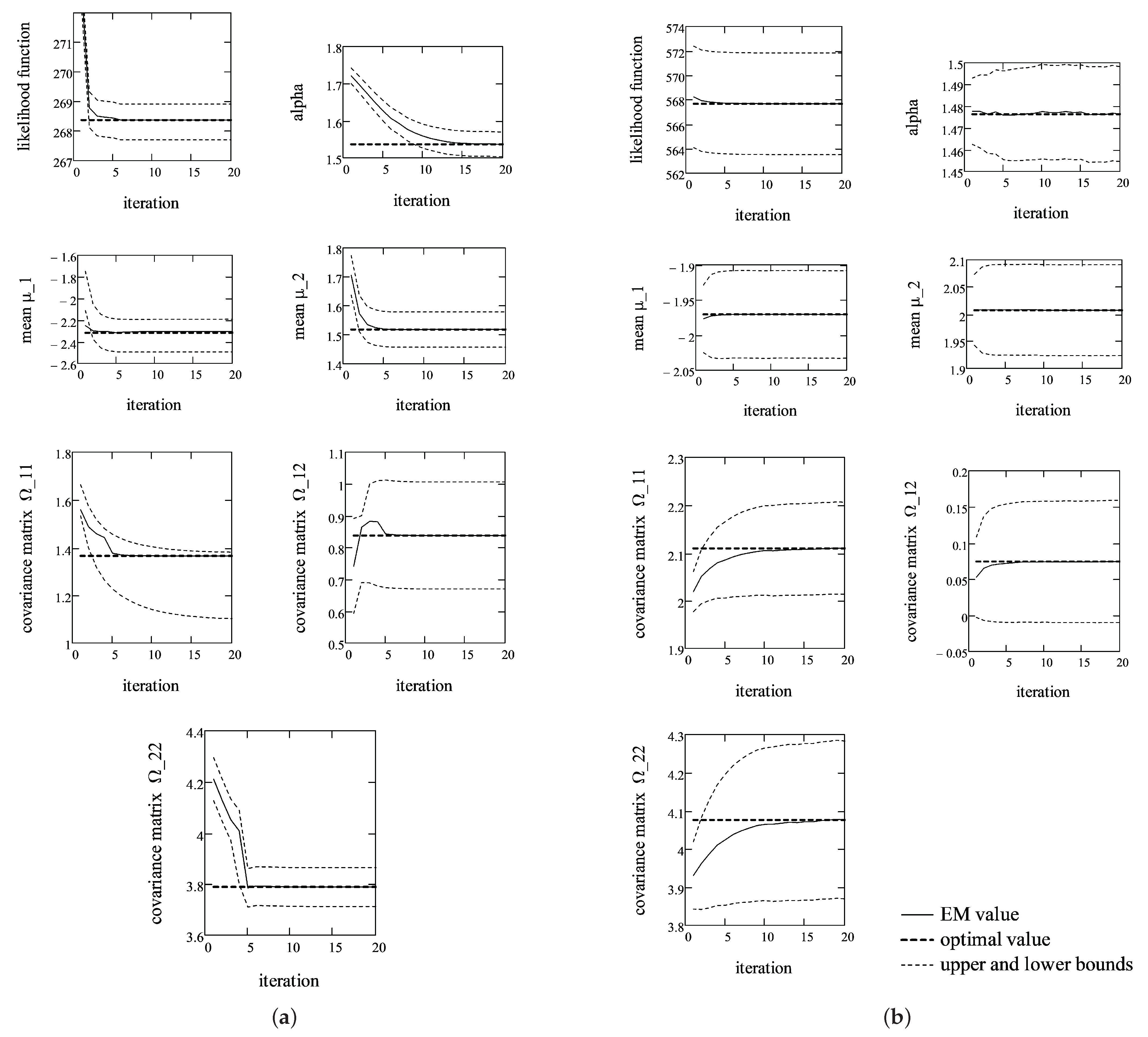
Then, for each two-dimensional vector, we estimated parameters of a bivariate, $\alpha$-stable distribution using the proposed EM algorithm and direct minimization of (3). We assume that the direct MLE method gives true estimates of a bivariate, $\alpha$-stable distribution. During each iteration, we registered EM estimates of all parameters until their values deviated from the previous estimate by no more than ${10}^{-8}$. Moreover, the terminal estimate was compared with the corresponding true value (obtained by direct method), and the statistical significance of differences was tested. It turns out that such precision ensures that there are no statistically significant differences between the true value and the corresponding terminal estimate. Thus, the analytical EM algorithm converged for all 100 samples. The averaged results are shown in Figure 1.

The averages of LLF and EM estimates are shown as solid lines for each iteration; corresponding values of direct MLE are dashed lines; and dotted lines are 95% confidence intervals calculated using the normal approximation. As shown in Figure 1, the convergence of the EM algorithm is rather fast independently of the sample size. The likelihood function and location parameter converged in 5–7 iterations; however, tail parameter $\alpha$ and covariance matrix converged only in slightly fewer than 20 iterations. This is not a surprise, because LLF is much more sensitive to changes in $\alpha$ and $\mathbf{\Omega }$. In the case of shorter samples ($K=50$, Figure 1a), the average LLF converged to 268.38, which is equal to the average value of the direct method (the average is calculated from $M=100$ estimates of random two-dimensional samples). The corresponding values of other parameters on average converged to $\widehat{\alpha }=1.538$, $\widehat{\mathbf{\mu }}=\left(\begin{array}{c}-2.305\\ 1.519\end{array}\right)$ and $\widehat{\mathbf{\Omega }}=\left(\begin{array}{cc}1.366& 0.838\\ 0.838& 3.789\end{array}\right)$. If the samples were of length $K=100$ (Figure 1b), then the average LLF converged to 567.69, which on average is the same as that obtained using the direct MLE method. The corresponding values of distribution parameters on average converged to $\widehat{\alpha }=1.476$, $\widehat{\mathbf{\mu }}=\left(\begin{array}{c}-1.97\\ 2.01\end{array}\right)$ and $\widehat{\mathbf{\Omega }}=\left(\begin{array}{cc}2.11& 0.075\\ 0.075& 4.076\end{array}\right)$. The presented results illustrate the convergence of the created EM algorithm with respect to (3), (5) and (6).

It must be noted that the same convergence (as seen in the average case) was observed in each of the 100 cases, too. This means that, independently of the sample selected, the EM estimates always converged to the values obtained by the direct MLE method.

Finally, the likelihood ratio test was performed for all simulated datasets, where a particular LLF value in each case was compared with the empirical distribution function of the LLF with original parameters $\alpha$, $\mathbf{\mu }$ and $\mathbf{\Omega }$. If we set the significance level p to 0.01, then, according to the likelihood ratio test (Section 2.4), the empirical probability should be within the interval $\left(\frac{p}{2},1-\frac{p}{2}\right)$, i.e., $(0.005,0.995)$. In this case, we cannot reject the hypothesis that the simulated data fit a symmetrical, multivariate $\alpha$-stable distribution with given parameters $\alpha$, $\mathbf{\mu }$ and $\mathbf{\Omega }$. During our experiment, there were no cases when the hypothesis could be rejected.

It must be noted that analytical EM algorithm is 30 times faster than the direct MLE algorithm and could be used in practice.

3.2. Stock Market Data

In the previous section, we showed that the EM algorithm is fast and converges in approximately 20 iterations independently of the length of the dataset. Theoretically, if the datasets are symmetrically distributed with the same parameter $\alpha$, then the EM algorithm should converge quickly and the parameter estimates should converge to true values. We now show a practical example with real stock price data from Yahoo [46]. The algorithm was applied to daily stock returns of four companies, AAPL, TSLA, LUMIN and ATnT, collected during 2019–2021. This experiment dataset consisted of four-dimensional vectors of length $K=545$.

First, we investigate the marginal characteristics of the underlying returns (AAPL, TSLA, LUMIN and ATnT).

Table 1. Marginal characteristics of stock returns.

Characteristics		AAPL	TSLA	LUMIN	ATnT
	mean, ${\mathbf{\mu }}^0$	0.00187	0.00329	−0.00072	−0.00015
	median	0.00344	0.00333	0.00076	0.00076
	std	0.02283	0.04772	0.02988	0.01630
empirical	min	−0.09481	−0.26731	−0.15462	−0.11208
	max	0.08864	0.23701	0.21938	0.06702
	skewness	−0.48712	−0.36526	−0.15063	−1.13504
	kurtosis	3.17	4.58	9.05	7.98
	$\alpha$	1.51272	1.53694	1.67748	1.61343
	$\beta$	−0.13074	0.06615	−0.28920	−0.09083
$\alpha$-stable	$\mathbf{\mu }$	0.00327	0.00314	0.00144	0.00058
	$\sigma$	0.01143	0.02377	0.01546	0.00816
	A-D	0.662	0.305	0.253	0.214

presents the empirical characteristics and estimates of marginal $\alpha$-stable distributions.

As we can see, the mean returns of AAPL and TSLA were positive, while those of LUMIN and ATnT were negative, which indicates that prices of the first two were mostly increasing during the period analyzed, while the prices of the latter two mainly decreased. We use the vector of empirical means as one of input parameters ${\mathbf{\mu }}^0$ for the EM algorithm. Furthermore, negative skewness and kurtosis above three indicate that the marginal empirical distributions for all the assets deviate from normality/symmetries. This assumption is supported by the fact that estimated marginal parameters $\alpha$ are different from two and $\beta$ are different from zero. Moreover, Anderson–Darling statistics (A-D) that is calculated for each sample, if we assume an $\alpha$-stable distribution with given parameter estimates, indicate that we cannot reject the non-parametric hypothesis about data fitness with $\alpha$-stable distribution. It must be noted that $\alpha$ was slightly different for all assets analyzed, which indicates that we deviated from theoretical assumptions, but not too far.

Next, in

Table 2. Correlation and covariance of stock returns.

	Correlation				Covariance, ${\mathbf{\Omega }}^0$
	AAPL	TSLA	LUMIN	ATnT	AAPL	TSLA	LUMIN	ATnT
AAPL	1	0.4919	0.2864	0.3243	0.00052	0.00054	0.00019	0.00012
TSLA	0.4919	1	0.1822	0.1772	0.00054	0.00228	0.00026	0.00014
LUMIN	0.2864	0.1827	1	0.5149	0.00019	0.00026	0.00089	0.00025
ATnT	0.3243	0.177	0.5149	1	0.00012	0.00014	0.00025	0.00027

, we show the correlation and covariance among the assets analyzed.

The covariance matrix is input parameter ${\mathbf{\Omega }}^0$ for the EM algorithm, while the correlation allows us to understand how strong the linear relation between variables is. As can be seen, stock returns are positively but weakly correlated. Only ATnT and LUMIN have correlations above 0.5.

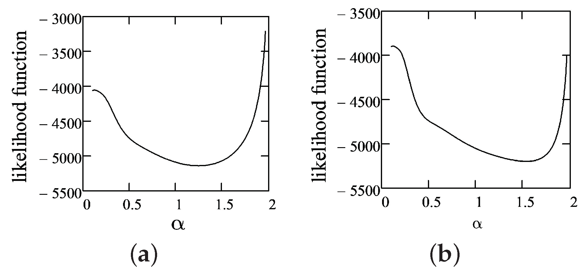
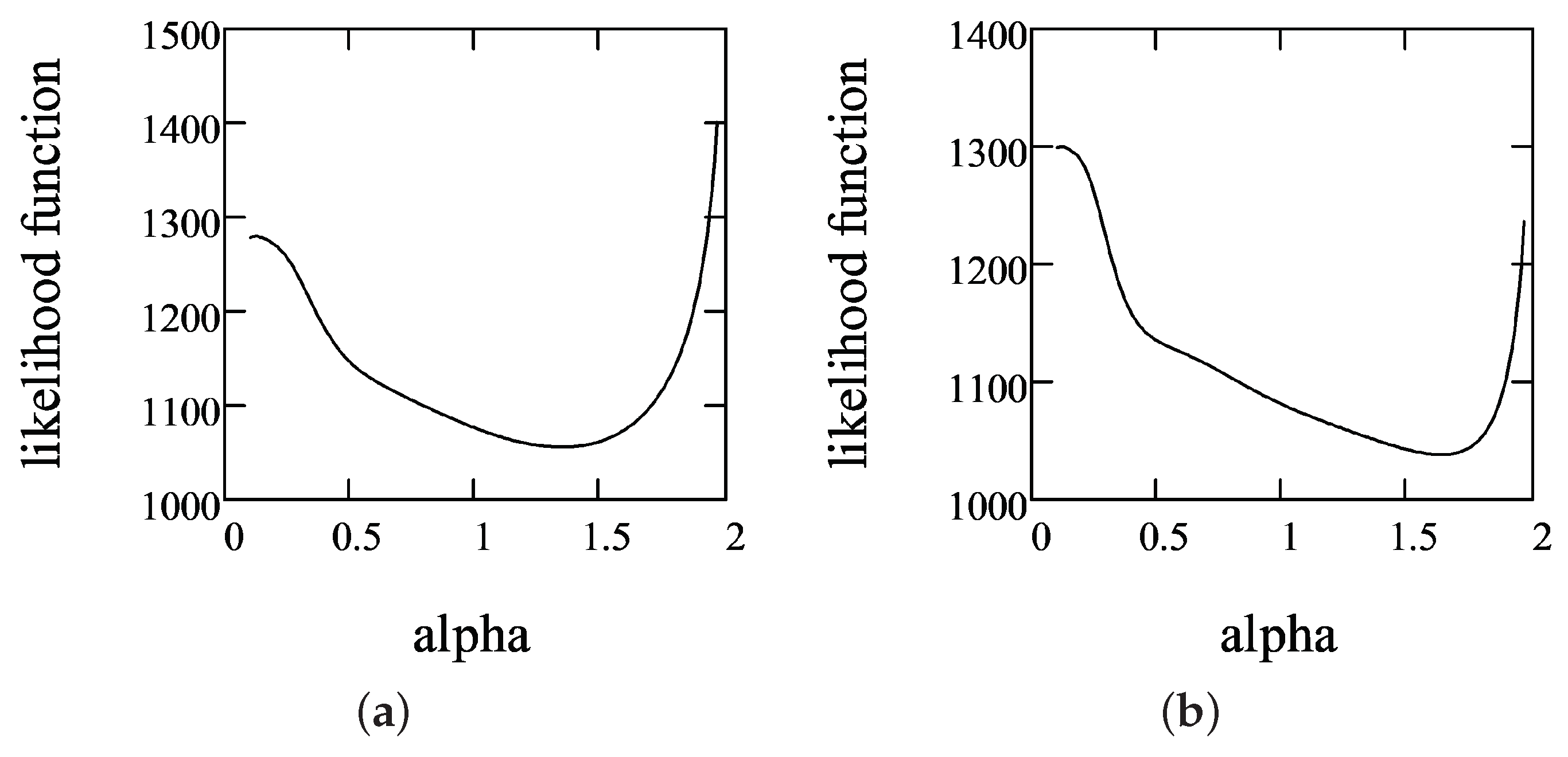
Figure 2 shows that the LLF for fixed $\mathbf{\mu }$ and $\mathbf{\Omega }$ is unimodal with respect to the tail parameter $\alpha$. Moreover, this property was observed in all iterations.

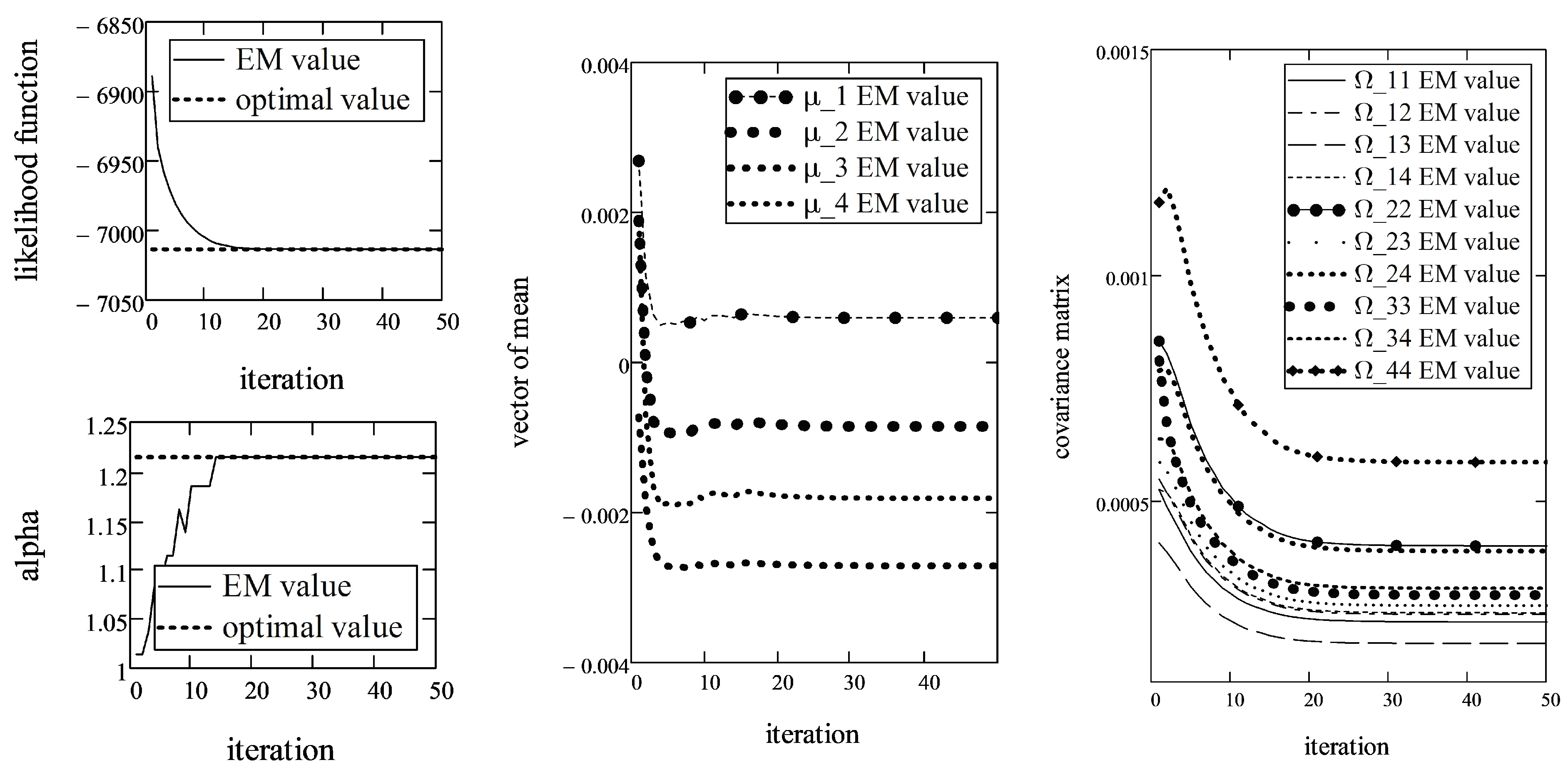
Therefore, the application of the golden section search method is reasonable in order to minimize LLF with respect to $\alpha$. In this case, the EM algorithm converged in fewer than 30 iterations. Figure 3 shows the dependence of the id of iterations and LLF and the estimates of parameters $\alpha$, $\mu$ and $\mathbf{\Omega }$.

As it may be observed, the convergence is slightly slower in the stock data case compared with the simulated datasets. Such behavior might be due to the fact that the real datasets are asymmetric and have different marginal parameters $\alpha$. However, this assumption is not supported by any kind of experiments yet.

According to results of the EM algorithm, the parameter estimates of the multivariate $\alpha$-stable distribution for stock data are as follows:

${\widehat{\alpha }}^{14}=1.51459$,

$${\widehat{\mathbf{\mu }}}^{27}=\left(\begin{array}{c}0.0024\\ 0.0044\\ 0.0012\\ 0.0007\end{array}\right)\mathrm{and}{\widehat{\mathbf{\Omega }}}^{28}=\left(\begin{array}{cccc}0.000083& 0.00007& 0.000024& 0.000011\\ 0.00007& 0.000351& 0.000035& 0.000015\\ 0.000024& 0.000035& 0.00014& 0.000034\\ 0.000011& 0.000015& 0.000034& 0.000041\end{array}\right),$$

while the terminal value of the LLF${}^{29}$ function was equal to $-5193.62$. The subscript above indicates the iteration at which the parameter estimate converged. As we can see, the LLF converged after 29 iterations so we say that the algorithm converged after 29 iterations too. The estimate ${\widehat{\alpha }}^{14}=1.51459$ confirms the assumption (from literature) that $\alpha$ for stock returns from developed markets is above 1.5.

We demonstrated that, even if the data are not purely symmetrically distributed, EM converges quickly and allows us to obtain ML estimates of parameters of multivariate $\alpha$-stable random variables. However, it was not shown yet how good the the estimation is. Now, let us show the likelihood ratio test as a goodness-of-fit test.

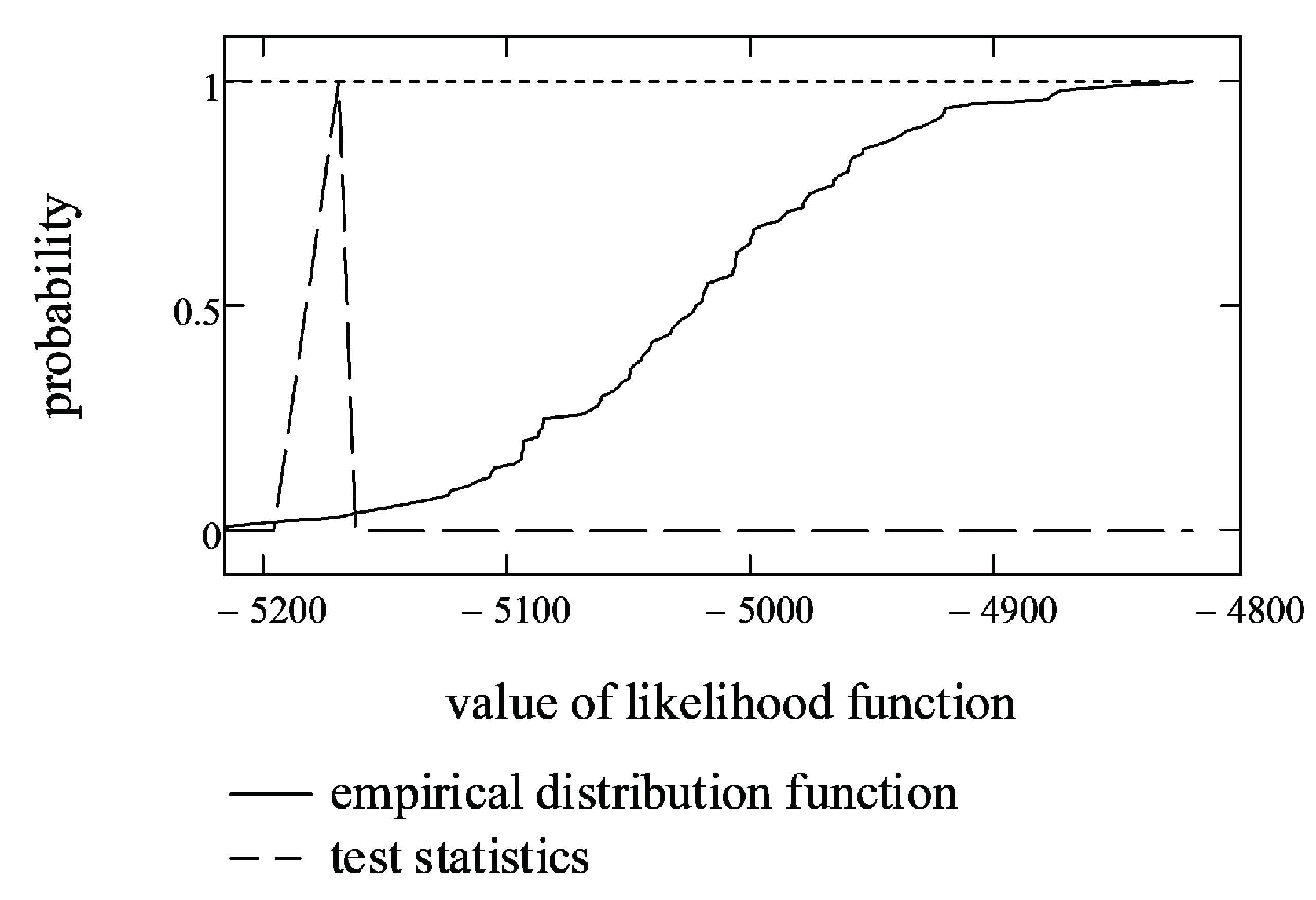
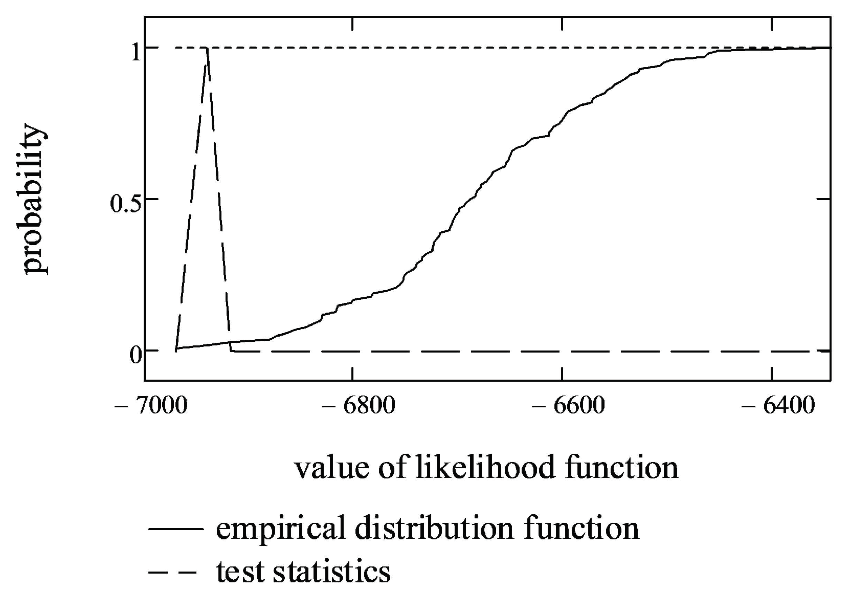
First, $M=100$ four-dimensional testing samples with estimated parameters ${\widehat{\alpha }}^{14}$, ${\widehat{\mathbf{\mu }}}^{27}$ and ${\widehat{\mathbf{\Omega }}}^{28}$ were generated, and LLF values for each sample were calculated. Then, the empirical distribution function from LLF values was constructed (shown as a solid line in Figure 4).

Secondly, the empirical probability that the random value of LLF is less than or equal to the terminal value of $LLF=-5193.62$ (test statistics) was calculated (shown as a dashed line in Figure 4). In the case of stock market data, the empirical probability of the test statistics was equal to 0.020927.

Finally, if we set the significance level to 0.01, according to the likelihood ratio test, this probability is within the interval (0.005, 0.995). This means that we cannot reject the hypothesis that the data fit a multivariate, symmetric, $\alpha$-stable distribution with parameters ${\widehat{\alpha }}^{14}$, ${\widehat{\mathbf{\mu }}}^{27}$ and ${\widehat{\mathbf{\Omega }}}^{28}$.

3.3. AIS Data Modeling

In a similar manner, we give an example of the analysis of data from the Australian Institute of Sport (AIS), examined in [47] (the database is often used for statistical calculations). This dataset contains various biomedical measurements (body fat (Bfat, %), lean body mass (LBM, kg), height (Ht, cm) and total weight (Wt, kg)) of a group of female Australian athletes [48]. In this experiment, the data consisted of a four-dimensional vector of length $K=100$.

Table 3. Marginal characteristics of Australian Institute of Sport (AIS) data.

Characteristics		Bfat, %	LBM, kg	Ht, cm	Wt, kg
	mean ${\mathbf{\mu }}^0$	17.85	54.89	174.59	67.34
	median	17.94	54.92	175	68.05
	std	5.45	6.92	8.24	10.92
empirical	min	8.07	34.36	148.9	37.8
	max	35.52	72.98	195.9	96.3
	skewness	0.35	−0.31	−0.57	−0.17
	kurtosis	−0.04	0.54	1.32	0.20
	$\alpha$	1.9358	1.9145	1.6858	1.9999
	$\beta$	0.9999	−0.9999	−0.5211	−0.9993
$\alpha$-stable	$\mathbf{\mu }$	17.54	55.39	175.67	67.34
	$\sigma$	3.716	4.692	4.873	7.679
	A-D	0.563	0.554	0.180	0.395

gives the empirical characteristics and estimates of marginal $\alpha$-stable distributions for female athletes.

As shown in Table 3, the data are not leptokurtic (kurtosis < 3), which means that the data are light-tailed or lack outliers. Moreover, the negative kurtosis of Bfat indicates that its distribution has a lighter tail than the normal distribution. Bfat, LBM and Wt are fairly symmetrical, because their skewness is between −0.5 and 0.5. All mentioned observations indicate that Bfat, LBM and Wt could be normally distributed. This assumption is supported by goodness-of-fit statistics (A-D statistics), which, being less that 2, indicate that Bfat, LBM and Wt are $\alpha$-stable distributed with $\alpha \to 2$ (normal distribution). However, the marginal estimate of parameter $\alpha$ for Ht is equal to 1.6858, and we cannot state that the four-dimensional vector is distributed by a multivariate normal distribution anymore. That is why we proceed with the estimation of parameters of the multivariate $\alpha$-stable distribution. If the terminal $\alpha$ of the EM algorithm turned out to be close to 2, then we would run a test for multivariate normality.

Next, we give estimates of correlation and covariance matrices for AIS data (see

Table 4. Correlation and covariance of AIS data.

	Correlation				Covariance, ${\mathbf{\Omega }}^0$
	Bfat, %	LBM, kg	Ht, cm	Wt, kg	Bfat, %	LBM, kg	Ht, cm	Wt, kg
Bfat, %	1	0.4062	0.4431	0.7249	29.73	15.33	19.91	43.15
LBM, kg	0.4062	1	0.7083	0.9208	15.33	47.92	40.41	69.57
Ht, cm	0.4431	0.7083	1	0.7087	19.91	40.41	67.93	63.76
Wt, kg	0.7249	0.9208	0.7087	1	43.15	69.57	63.76	119.15

).

As shown in Table 4, AIS data are strongly correlated, with the exception of Bfat, which correlates weakly with LBM and Ht. When we initiated the EM algorithm (in the same vein as in previous section), we used the vector of means as the initial value of ${\mathbf{\mu }}^0$ and the covariance matrix as the initial value of ${\mathbf{\Omega }}^0$. Similar to Figure 2, in Figure 5, we show that the LLF for a fixed $\mathbf{\mu }$ and $\mathbf{\Omega }$ is unimodal with respect to the stability parameter $\alpha$.

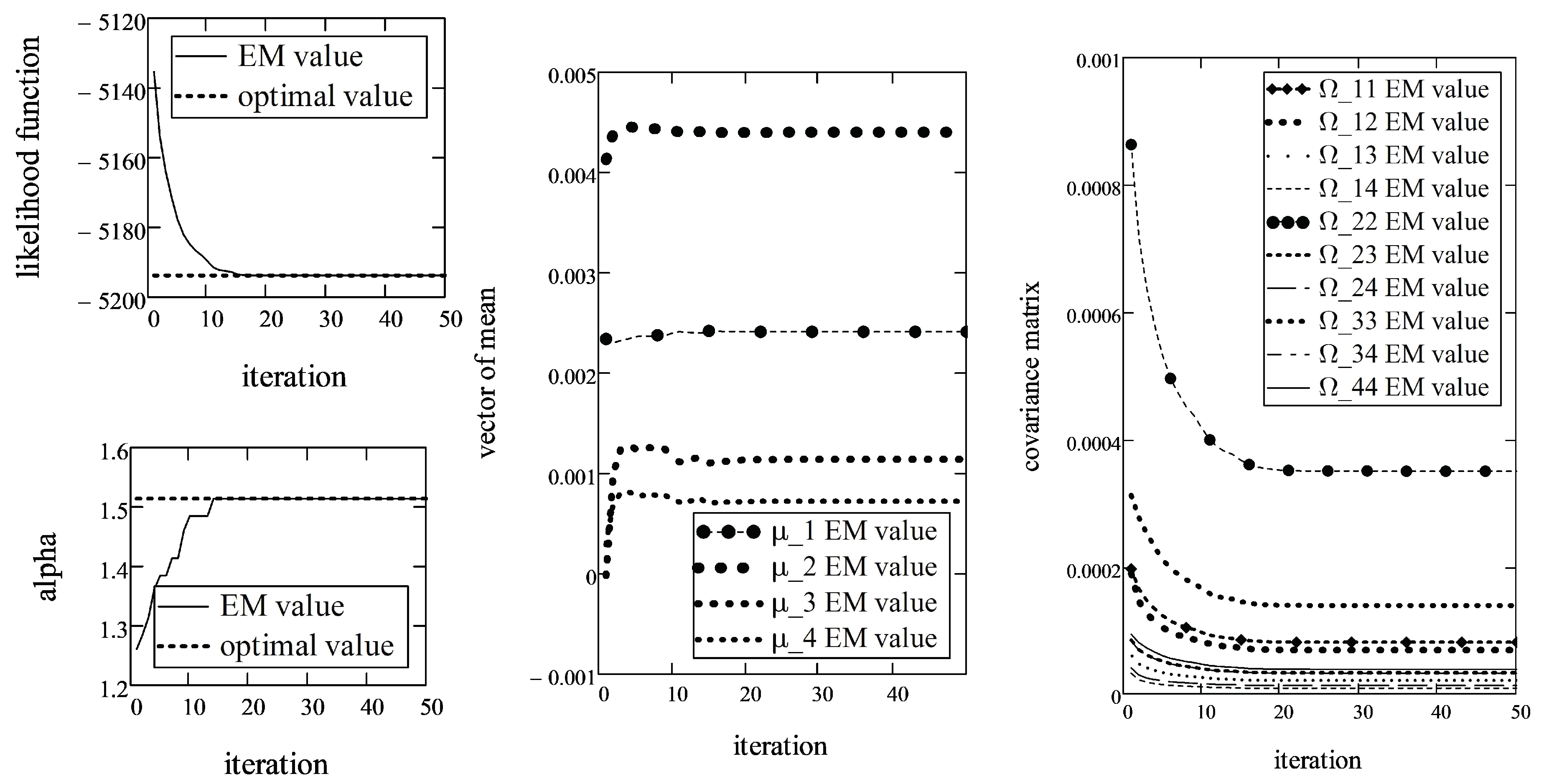
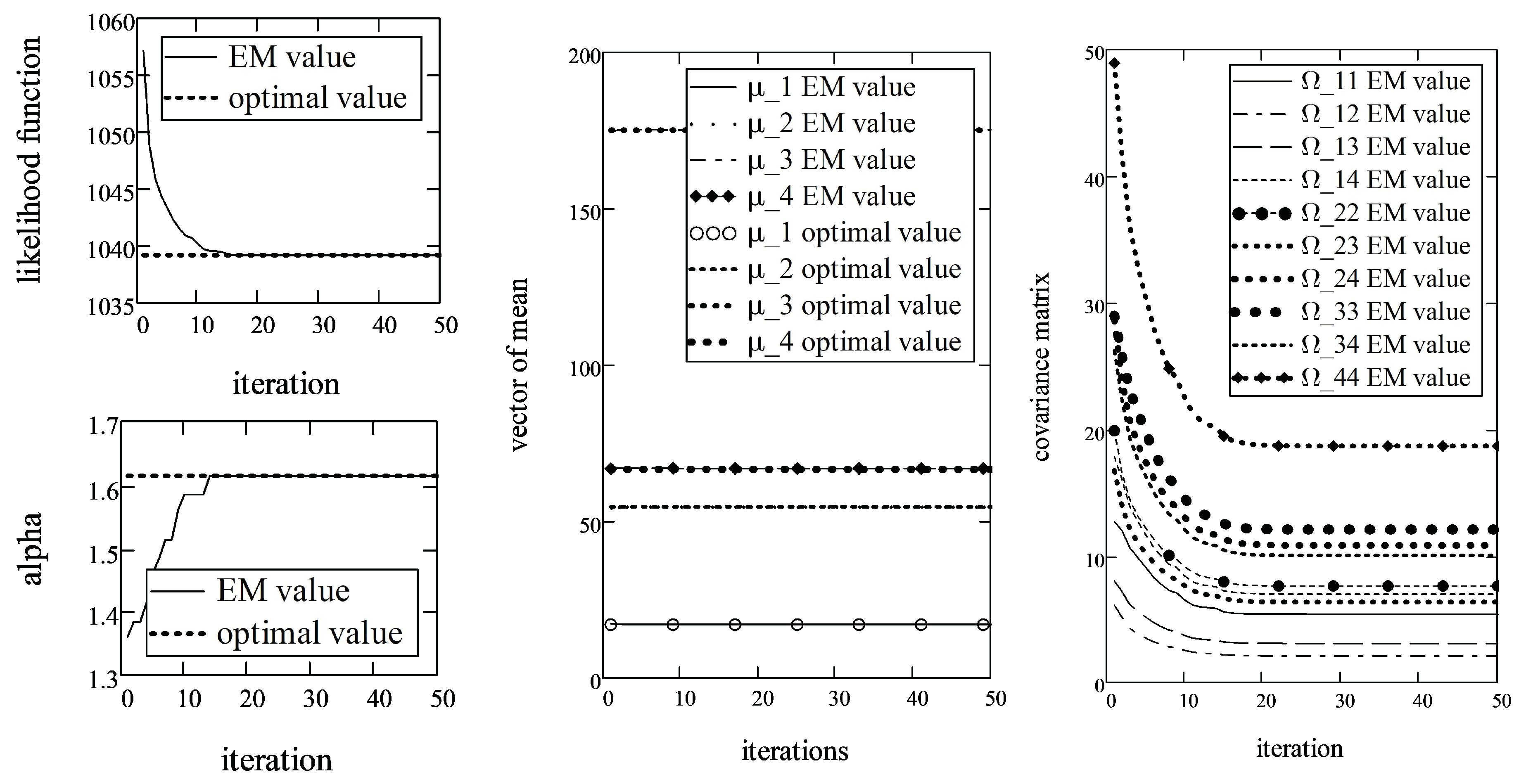
Using the EM algorithm described in this paper, the LLF value and parameter estimates were registered during 100 iterations (see Figure 6).

The optimal value of the parameter $\alpha$ was obtained after 14 iterations. However, the EM algorithm converged with respect to the mean and covariance matrix, respectively, after 40 and 47 (slightly more than in stock case) iterations. From the figure of parameters $\mathbf{\mu }$ (middle column in Figure 6), it may appear that the convergence of the location parameter was achieved very early; however, as the initial value of $\mathbf{\mu }$ was luckily selected very close to true value, the oscillations were very small. The greatest absolute deviation of $\mathbf{\mu }$ in sequential iterations was in the interval $[-0.00071,0.00339]$ and visually cannot be seen. According to the EM algorithm, the estimates of the parameters of the multivariate $\alpha$-stable distribution for AIS data are as follows:

${\widehat{\alpha }}^{14}=1.61459$,

$${\widehat{\mathbf{\mu }}}^{40}=\left(\begin{array}{c}17.61\\ 55.24\\ 175.33\\ 67.38\end{array}\right)\mathrm{and}{\widehat{\mathbf{\Omega }}}^{47}=\left(\begin{array}{cccc}5.49& 2.19& 3.17& 7.07\\ 2.19& 7.69& 6.44& 10.91\\ 3.17& 6.44& 12.16& 10.12\\ 7.07& 10.91& 10.12& 18.76\end{array}\right),$$

while the terminal value of the LLF${}^{27}$ function is equal to $1039.22$. It is interesting to note that the sample size in the AIS data case was five times smaller than that of the stock data; however, the number of iterations was nearly double.

As we can see again, terminal $\widehat{\alpha }=1.61459$ is not very different form the smallest marginal $\alpha =1.685812$. Furthermore, the estimated $\widehat{\alpha }$ was different from two, which is why we can reject the hypothesis about the multivariate normality of AIS data.

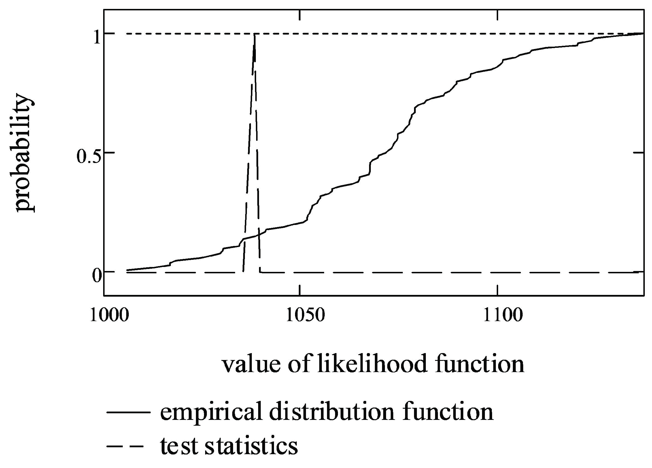
Now, let us show a likelihood ratio test in the same manner as in the previous section. First, we constructed empirical distribution function from LLF values with parameters ${\widehat{\alpha }}^{14}$, ${\widehat{\mathbf{\mu }}}^{40}$ and ${\widehat{\mathbf{\Omega }}}^{47}$ (shown as a solid line in Figure 7).

Secondly, we calculated the empirical probability that a random value of LLF is less than or equal to the terminal value $LLF=1039.22$ (shown as a dashed line in Figure 7). In the case of AIS data, the empirical probability is equal to 0.3662.

Finally, we cannot reject the hypothesis that AIS data fit a symmetric multivariate $\alpha$-stable distribution with parameters ${\widehat{\alpha }}^{14}$, ${\widehat{\mathbf{\mu }}}^{40}$ and ${\widehat{\mathbf{\Omega }}}^{47}$ because this probability is within the interval (0.005, 0.995).

3.4. Cryptocurrency Data

Finally, we show how the EM algorithm can be applied to estimate the parameters of a four-dimensional cryptocurrency dataset. As an example, Bitcoin, Ethereum, Ripple and ADA (during 2019–2021 [46]) were used. Hence, the length of the vector is $K=791$ (exchanges operate 24/7 the whole year).

Table 5. Marginal characteristics of cryptocurrency returns.

Characteristics		Bitcoin	ETH	XRP	ADA
	mean ${\mathbf{\mu }}^0$	0.0024	0.0017	−0.0013	0.0026
	median	0.0018	0.0017	−0.0007	0.0027
	std	0.0409	0.0523	0.0574	0.0586
empirical	min	−0.5771	−0.7281	−0.7286	−0.6546
	max	0.1580	0.2073	0.3556	0.2441
	skew	−3.53	−3.72	−2.86	−1.67
	kurtosis	52.01	49.05	43.20	20.94
	$\alpha$	1.3802	1.5239	1.3367	1.6013
	$\beta$	0.0827	0.0566	−0.0172	0.0904
$\alpha$-stable	$\mathbf{\mu }$	0.0019	0.0029	−0.0001	0.0019
	$\sigma$	0.0159	0.0231	0.0190	0.0298
	A-D	0.698	0.799	0.447	0.599

gives empirical characteristics and estimates of marginal $\alpha$-stable distributions of four cryptocurrencies.

There is no big surprise that the characteristics of cryptocurrency data are different from those analyzed in Section 3.2 and Section 3.3. The first obvious things that are very different from the previous sections are the skewness and kurtosis. The negative skewness is nearly twice greater than for stocks and AIS data, while the kurtosis is extremely large and exceeds 20. Such a composition indicates that we should expect fat left tails, i.e., $\alpha \to 1$ and $\beta \to -1$. However, marginal estimates of the $\alpha$-stable distribution show that such an assumption is not completely true. Parameter $\beta$ is mainly close to 0, which indicates fair symmetry of the tails. Moreover, marginal $\alpha$s are not as extreme as expected, but they are significantly different from stocks and AIS data.

Next, in

Table 6. Correlation and covariance of cryptocurrency returns.

	Correlation				Covariance, ${\mathbf{\Omega }}^0$
	Bitcoin	ETH	XRP	ADA	Bitcoin	ETH	XRP	ADA
Bitcoin	1	0.8531	0.5667	0.7081	0.00172	0.00183	0.00133	0.00169
ETH	0.8532	1	0.6344	0.8103	0.00183	0.00274	0.00191	0.00249
XRP	0.5666	0.6344	1	0.5892	0.00133	0.00191	0.00330	0.00198
ADA	0.7081	0.8103	0.5892	1	0.00169	0.00249	0.00198	0.00344

, we check for empirical correlation and covariance.

As we can see, cryptocurrencies are average (above 0.5) to strongly (above 0.8) correlated, which indicates that there are high chances that the prices of underlying assets will move in the same direction. Such a portfolio would have a higher risk than a less correlated one.

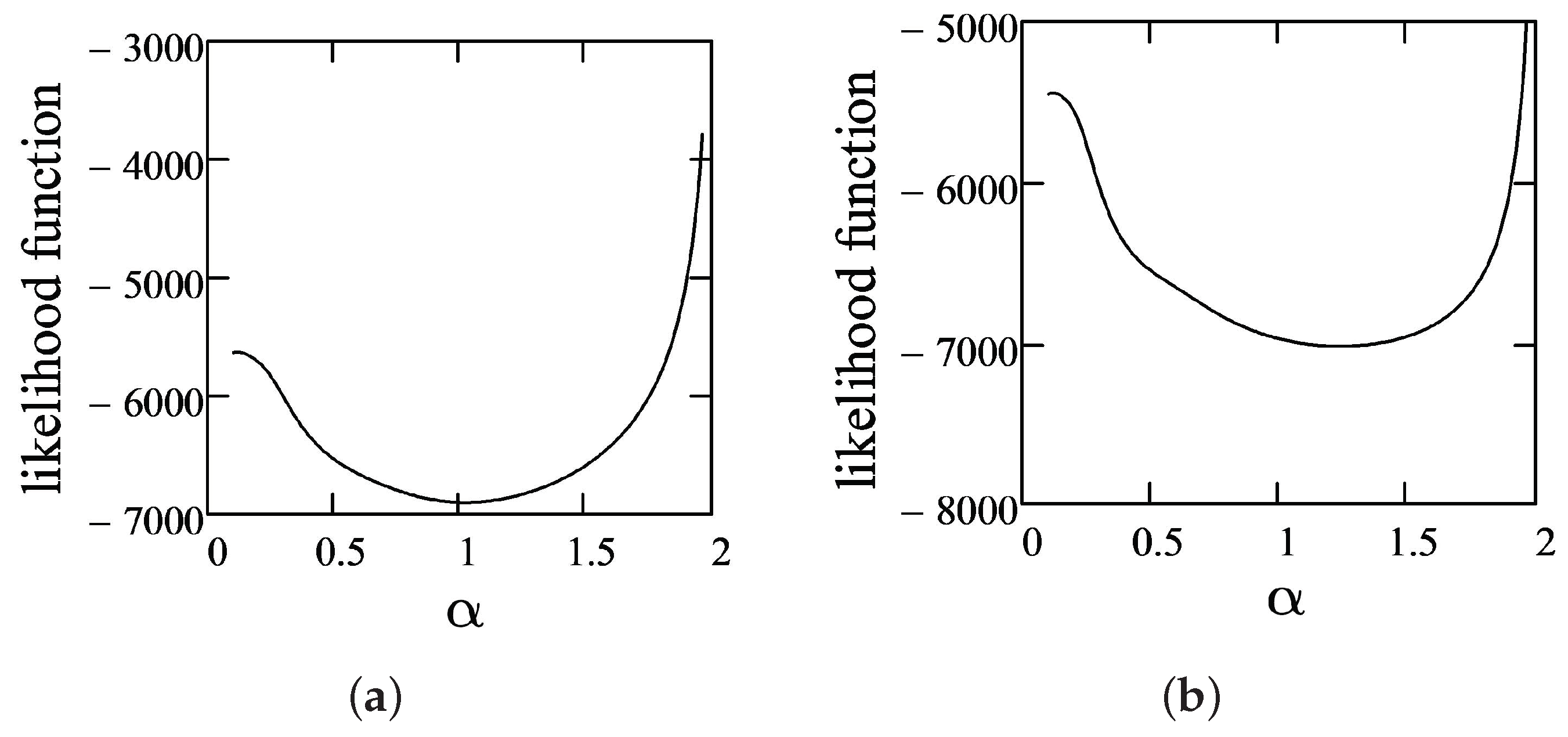
Next, we ran the EM algorithm to estimate the parameters of the multivariate $\alpha$-stable distribution. There is no surprise that the LLF for fixed $\mathbf{\mu }$ and $\mathbf{\Omega }$ is unimodal with respect to the stability parameter $\alpha$ (see Figure 8).

Using the EM algorithm, the LLF value and parameter estimates were registered for the first 100 iterations. However, the convergence conditions were reached much more quickly (see Figure 9).

Figure 9 shows that LLF and parameter estimates by the EM algorithm converge to the optimal maximum likelihood value after 50 iterations. The number of iterations is similar to the case of the AIS data case.

The estimates of parameters of a multivariate $\alpha$-stable distribution for cryptocurrency data are as follows: ${\widehat{\alpha }}^{14}=1.21459$,

$${\widehat{\mathbf{\mu }}}^{39}=\left(\begin{array}{c}0.00060\\ -0.00084\\ -0.00269\\ -0.00179\end{array}\right)\mathrm{and}{\widehat{\mathbf{\Omega }}}^{36}=\left(\begin{array}{cccc}0.000236& 0.000252& 0.000188& 0.000256\\ 0.000252& 0.000404& 0.000273& 0.000392\\ 0.000188& 0.000273& 0.000295& 0.000310\\ 0.000256& 0.000392& 0.000310& 0.000589\end{array}\right),$$

while the terminal value of the LLF${}^{50}$ function is equal to $-7013.09$. By contrast to the stock market, the estimate of parameter $\alpha$ for cryptocurrency is below 1.5, which is not a surprise.

Now, let us show a likelihood ratio test in the same manner as in the two previous sections. First, we constructed an empirical distribution function from LLF values with parameters ${\widehat{\alpha }}^{14}$, ${\widehat{\mathbf{\mu }}}^{39}$ and ${\widehat{\mathbf{\Omega }}}^{36}$ (shown as a solid line in Figure 10).

Secondly, we calculated the empirical probability that a random value of LLF is less than or equal to the terminal value $LLF=-7013.09$ (shown as dashed line in Figure 10). In the case of cryptocurrency data, the empirical probability is equal to 0.08119 and is near the lower bound of non-rejection (0.005, 0.995) region. However, we cannot reject hypothesis that cryptocurrency data fits multivariate symmetric $\alpha$-stable distribution with parameters ${\widehat{\alpha }}^{14}$, ${\widehat{\mathbf{\mu }}}^{39}$ and ${\widehat{\mathbf{\Omega }}}^{36}$.

3.5. Recommendations

In the previous three sections, we demonstrate examples of how to estimate parameters of a multivariate $\alpha$-stable distribution using an analytical EM algorithm. In the case of stock data, the estimated tail parameter $\widehat{\alpha }$ of the multivariate case was very close to the smallest marginal $\alpha$ estimate (given in Table 1). Moreover, a similar situation was observed in AIS and cryptocurrency data. This gives us an idea of how to chose the initial ${\alpha }^0$ for applications of the EM algorithm in the future.

Furthermore, the estimate $\widehat{\mathbf{\mu }}$ in the case of stock data was more similar to the vector of medians or vector $\mathbf{\mu }$ of marginal estimates rather than the vector of empirical means. However, for AIS data, marginal empirical distributions were symmetrical (all empirical location parameters were very similar) so there was no difference if we chose a vector of empirical means, medians or marginal parameters $\mathbf{\mu }$ as the initial value for ${\mathbf{\mu }}^0$.

By summarizing two latest assumptions, we can recommend one to chose the smallest marginal $\alpha$, vector of marginal $\mathbf{\mu }$ parameters (or medians) and covariance matrix as initial values for the EM algorithm. This could increase efficiency and reduce the number of iterations required to converge.

By summarizing the findings from the last four sections, we can give the following recommendations for the implementation of an analytical EM algorithm:

• Check for empirical characteristics of datasets. The vectors of means or medians can be used as initial values for ${\mathbf{\mu }}^0$, and the covariance matrix as an input parameter for ${\mathbf{\Omega }}^0$.
• If estimates of a marginal $\alpha$-stable distribution are available, then choose the minimal $\alpha$ as the initial value of ${\alpha }^0$ and the vector of location parameters as ${\mathbf{\mu }}^0$.
• Run the EM algorithm and check for convergence.
• (Optional) When one or more parameter estimates converge, stop updating them and optimize only with respect to parameters that did not converge. However, such a modification may cause the algorithm to get stuck in a local minimum.
• Use the likelihood ratio test to check the goodness-of-fit.

4. Discussion and Conclusions

Today, the research of distributions related to $\alpha$-stable ones, including sub-Gaussian vectors, is more relevant, because they often occur in the analysis of economic data, information flows along computer networks, cryptocurrency markets, etc. The statistical maximum likelihood approach is constructed by the analytical EM algorithm in this paper, which allows us to estimate the parameters of the symmetric multivariate $\alpha$-stable distribution with high precision. Computational experiments showed that multivariate $\alpha$-stable distribution parameter estimates, obtained by the developed numerical method, are statistically adequate, because, after a certain number of iterations, the value of the likelihood function and estimates of the parameters converged to their corresponding (“true”) values. However, due to the fact that real data are often asymmetric, it is very important to perform goodness-of-fit tests. The proposed likelihood ratio test (for assessment of the goodness-of-fit) showed that the data fit a multivariate $\alpha$-stable model well with obtained estimates in all three cases analyzed (stock market data, biomedical measurements data and cryptocurrency data). In future research, this test could be compared with other multivariate goodness-of-fit tests, e.g., the one proposed in [34] or based on characteristic functions [32].

Moreover, it is more important to make sure that the methodology is robust with respect to the asymmetry and the fact that marginal $\alpha$s in real data are different. This is also the future trend of our research.

Furthermore, in the Results Section, we emphasized that the number of iterations is nearly independent of sample size; however, the duration of calculations (real CPU time) is highly dependent on that. This is due to the fact that the likelihood function is sample dependent. We plan (in the near future) to implement parallel summation in LLF and parallel quadrature integration to reduce overall processing time.

Finally, it must be noted that the analytical EM algorithm is 30 times faster than the regular ML algorithm and could be very useful in practice. However, it is currently not available in R or Python, where the stochastic EM algorithm is already implemented.

References

- Janicki, A.; Weron, A. Simulation and Chaotic Behavior of α-Stable Stochastic Processes; Marcel Dekker: New York, NY, USA, 1993. [Google Scholar]
- Rachev, S.T.; Mittnik, S. Stable Paretian Models in Finance; Wiley: New York, NY, USA, 2000. [Google Scholar]
- Samorodnitsky, G.; Taqqu, M.S. Stable Non-Gaussian Random Processes. Stochastic Models with Infinite Variance; Chapman & Hall: New York, NY, USA, 1994. [Google Scholar]
- Belov, I.; Kabašinskas, A.; Sakalauskas, L. A study of stable models of stock markets. Inf. Technol. Control. 2006, 35, 34–56. [Google Scholar]
- Kabasinskas, A.; Rachev, S.; Sakalauskas, L.; Sun, W.; Belovas, I. Stable Paradigm in Financial Markets. J. Comput. Anal. Appl. 2009, 11, 642–688. [Google Scholar]
- Bertocchi, M.; Giacometti, R.; Ortobelli, S.; Rachev, S.T. The impact of different distributional hypothesis on returns in asset allocation. Financ. Lett. 2005, 3, 17–27. [Google Scholar]
- Hoechstoetter, M.; Rachev, S.Z.; Fabozzi, F.J. Distributional Analysis of the Stocks Comprising the DAX 30. Probab. Math. Stat. 2005, 25, 363–383. [Google Scholar]
- Fielitz, B.D.; Smith, E.W. Asymmetric stable distributions of stock price changes. J. Am. Stat. Assoc. 1972, 67, 813–814. [Google Scholar] [CrossRef]
- Kabasinskas, A.; Sakalauskas, L.; Sun, E.W.; Belovas, I. Mixed-stable models for analyzing high-frequency financial data. J. Comput. Appl. 2012, 14, 1210–1226. [Google Scholar]
- Sakalauskas, L.; Kalsyte, Z.; Vaiciulyte, I.; Kupciunas, I. The application of stable and skew t-distributions in predicting the change in accounting and governance risk ratings. In Proceedings of the 8th International Conference Electrical and Control Technologies, Kaunas, Lithuania, 2–3 May 2013; pp. 53–58. [Google Scholar]
- Pele, D.T.; Wesselhöfft, N.; Härdle, W.K.; Kolossiatis, M.; Yatracos, Y.G. Phenotypic Convergence of Cryptocurrencies. IRTG 1792 Discussion Paper 2019–018. Available online: https://ssrn.com/abstract=3658082 (accessed on 21 January 2021).
- Kopa, M.; Kabašinskas, A.; Šutienė, K. A stochastic dominance approach to pension-fund selection. IMA J. Manag. Math. 2021, dpab002. [Google Scholar] [CrossRef]
- Nolan, J.P. Stable Distributions–Models for Heavy Tailed Data; Birkhäuser: Boston, MA, USA, 2007. [Google Scholar]
- Rachev, S.T.; Mittnik, S. Modeling asset returns with alternative stable distributions. Econom. Rev. 1993, 12, 261–330. [Google Scholar]
- Ravishanker, N.; Qiou, Z. Monte Carlo EM estimation for multivariate stable distributions. Stat. Probab. Lett. 1999, 45, 335–340. [Google Scholar] [CrossRef]
- Sakalauskas, L.; Vaiciulyte, I. Estimation of sub-Gaussian vector distribution by the Monte-Carlo Markov chain approach. J. Young Sci. 2014, 41, 104–107. [Google Scholar]
- Applebaum, D. L´evy Processes and Stochastic Calculus, 2nd ed.; Cambridge University Press: Cambridge, UK, 2009. [Google Scholar]
- Rachev, S.T.; Xin, H. Test for association of random variables in the domain of attraction of multivariate stable law. PRobability Math. Stat. 1993, 14, 125–141. [Google Scholar]
- Davydov, Y.; Paulauskas, V. On the estimation of the parameters of multivariate stable distributions. Acta Appl. Math. 1999, 58, 107–124. [Google Scholar] [CrossRef]
- Kring, S.; Rachev, S.T.; Höchstötter, M.; Fabozzi, F.J. Estimation of α-stable sub-Gaussian distributions for asset returns. In Risk Assessment: Decisions in Banking and Finance, Bol, G., Rachev, S.T., Würth, R., Eds.; Springer/Physika: Heidelberg, Germany, 2009; pp. 111–152. [Google Scholar]
- Nolan, J.P. Multivariate stable distributions: Approximation, estimation, simulation and identification. In A Practical Guide to Heavy Tails; Adler, R., Feldman, R.E., Taqqu, M., Eds.; Birkhäuser: Boston, MA, USA, 1998; pp. 509–525. [Google Scholar]
- Ogata, H. Estimation for multivariate stable distributions with generalized empirical likelihood. J. Econom. 2013, 172, 248–254. [Google Scholar] [CrossRef]
- Press, S.J. Estimation in univariate and multivariate stable distributions. J. Am. Stat. Assoc. 1972, 67, 842–846. [Google Scholar] [CrossRef]
- Daul, S.; DeGiorgi, E.; Lindskog, F.; McNeil, A. The grouped t-copula with an application to credit risk. RISK 2003, 16, 73–76. [Google Scholar] [CrossRef] [Green Version]
- Nolan, J.P. Multivariate elliptically contoured stable distributions: Theory and estimation. Comput. Stat. 2013, 28, 2067–2089. [Google Scholar] [CrossRef] [Green Version]
- Kouaissah, N.; Ortobelli, S.L. Multivariate Stochastic Dominance: A Parametric Approach. Econ. Bull. AccessEcon 2020, 40, 1380–1387. [Google Scholar]
- Teimouri, M.; Rezakhah, S.; Mohammadpur, A. Parameter Estimation Using the EM Algorithm for Symmetric Stable Random Variables and Sub-Gaussian Random Vectors. J. Stat. Theory Appl. 2018, 17, 439–461. [Google Scholar] [CrossRef] [Green Version]
- Fasano, G.; Franceschini, A. A multidimensional version of the Kolmogorov–Smirnov test. Mon. Not. R. Astron. Soc. 1987, 225, 155–170. [Google Scholar] [CrossRef]
- Justel, A.; Peña, D.; Zamar, R. A multivariate Kolmogorov-Smirnov test of goodness of fit. Stat. Probab. Lett. 1997, 35, 251–259. [Google Scholar] [CrossRef] [Green Version]
- Anderson, T.W.; Darling, D.A. Asymptotic theory of certain “goodness of fit” criteria based on stochastic processes. Ann. Math. Stat. 1952, 2, 193–212. [Google Scholar] [CrossRef]
- Matsui, M.; Takemura, A. Goodness-of-fit tests for symmetric stable distributions–Empirical characteristic function approach. TEST 2007, 17, 546–566. [Google Scholar] [CrossRef] [Green Version]
- Meintanis, S.G.; Ngatchou, W.J.; Taufer, E. Goodness-of-fit tests for multivariate stable distributions based on the empirical characteristic function. J. Multivar. Anal. 2015, 140, 171–192. [Google Scholar] [CrossRef]
- Sürücü, B. Goodness-of-Fit Tests for Multivariate Distributions. Commun. Stat. Theory Methods 2006, 35, 1319–1331. [Google Scholar] [CrossRef]
- McAssey, M.P. An empirical goodness-of-fit test for multivariate distributions. J. Appl. Stat. 2013, 40, 1120–1131. [Google Scholar] [CrossRef] [Green Version]
- Wilks, S.S. The Large-Sample Distribution of the Likelihood Ratio for Testing Composite Hypotheses. Ann. Math. Statist. 1938, 9, 60–66. [Google Scholar] [CrossRef]
- Sakalauskas, L. On the empirical Bayesian approach for the Poisson-Gaussian model. Methodol. Comput. Appl. Probab. 2010, 12, 247–259. [Google Scholar] [CrossRef]
- Le Cam, L.; Yang, G.L. Asymptotics in Statistics: Some Basic Concepts; Springer: New York, NY, USA, 2000. [Google Scholar]
- Bogdan, K.; Byczkowski, T.; Kulczycki, T.; Ryznar, M.; Song, R.; Vondracek, Z. Potential Analysis of Stable Processes and its Extensions; Springer: New York, NY, USA, 2009. [Google Scholar]
- Magnus, J.R.; Neudecker, H. Matrix Differential Calculus with Applications in Statistics and Econometrics; John Wiley & Sons Ltd.: New York, NY, USA, 1999. [Google Scholar]
- Burden, R.L.; Faires, J.D. Numerical Analysis; Brooks/Cole Cengage Learning: Boston, MA, USA, 2011. [Google Scholar]
- Stoer, J.; Bulirsch, R. Introduction to Numerical Analysis; Springer: New York, NY, USA, 2002. [Google Scholar]
- Casio Computer Co. Available online: http://keisan.casio.com/exec/system/1281279441 (accessed on 15 October 2019).
- Ehrich, S. On stratified extensions of Gauss-Laguerre and Gauss-Hermite quadrature formulas. J. Comput. Appl. Math. 2002, 140, 291–299. [Google Scholar] [CrossRef] [Green Version]
- Kovvali, N. Theory and Applications of Gaussian Quadrature Methods; Morgan & Claypool Publishers: San Rafael, CA, USA, 2012. [Google Scholar]
- Casella, G.; Berger, R.L. Statistical Inference, 2nd ed.; Duxbury Press: Pacific Grove, CA, USA, 2002. [Google Scholar]
- Yahoo Finance. Available online: http://finance.yahoo.com (accessed on 21 January 2021).
- Cook, R.D.; Weisberg, S. An Introduction to Regression Graphics; Wiley: New York, NY, USA, 1994. [Google Scholar]
- Smyth, G.K. Australasian Data and Story Library (OzDASL). Available online: http://www.statsci.org/data/oz/ais.txt (accessed on 12 June 2015).
Figure 1.
Average log-likelihood function (LLF) and average estimates of parameters in the case of : (a); and (b).
Figure 2.
LLF dependence on : (a) at the first iteration; and (b) at the last iteration for stock data.
Figure 3.
Dependence of the LLF, , and parameters on the number of iterations for and .
Figure 4.
The empirical distribution function of LLF and test statistics of the stock market data.
Figure 5.
LLF dependence on : (a) at the first iteration; and (b) at the last iteration for AIS data.
Figure 6.
Dependence of the LLF and parameters’ MLE on the number of EM iterations, , .
Figure 7.
The empirical distribution function of LLF and test statistics of AIS data.
Figure 8.
LLF dependence on : (a) at the first iteration; and (b) at the last iteration.
Figure 9.
Dependence of the LLF, , and parameters on the numbers of iterations with and .
Figure 10.
The empirical distribution function of LLF and test statistics of cryptocurrency data.