1. Introduction
In December 2019, the Chinese public health authorities informed the world about several cases of acute respiratory syndrome in Wuhan. By 7 Jan 2020, scientists had isolated a novel coronavirus from these patients not previously identified in humans, referred to as severe acute respiratory syndrome coronavirus 2 (SARS-CoV-2), the agent responsible for the later designated coronavirus disease 2019 (COVID-19) in February 2020, and the World Health Organization (WHO) declared a pandemic [
1,
2].
So far, we have been buying time looking for a balance between the overload of the hospitals and the economy until antivirals and vaccines are available. Every time stronger population restrictions are applied, a new wave appears because the trend of the disease is to infect people until most of them have been infected or vaccinated. In this sense, mathematical models have been remarkable tools for knowing in advance the appropriate time to enforce the population restrictions and distribute the hospital resources to face the new waves.
Several approaches have tried to mathematically model the transmission dynamics of COVID-19 using SIR and SEIR-type models [
3,
4,
5,
6,
7,
8,
9]. Other references, such as [
10,
11,
12,
13], moreover, consider asymptomatic infected individuals, most of the infected population, who play an important role in spreading the virus. One of the main advantages of these mathematical models is that different simulations can be carried out, allowing the study of a different variety of complex scenarios, although with limitations due to the many uncertainties regarding the disease.
One of the main parameters in the epidemiological models is the reproductive number (
), which quantifies the average of secondary cases generated from each infected person in a susceptible environment during an outbreak. Different studies have estimated that the
value in China at the beginning of the pandemic was between 2 and
. This means that, following [
14], the pandemic is not going to be controlled until we reach herd immunity, and it will be possible when the percentage
of the population will be immune, that is, recovered plus vaccinated. Thus,
for
and
for
. It has also been observed that
value drops sharply after the implementation of control measures against COVID-19 [
15] reducing the percentage to reach herd immunity.
Under a demographic point of view, Granada is a province in southern Spain with a population of
inhabitants, around 30% of the population live in the capital and the province has a population density of 73.5 people per km
2 [
16]. Compared with the province of Madrid with 829.6 people per km
2, the province of Granada has a low population density. Also, the percentage of accumulated infected between 1 May 2020 and 1 June 2020 was [2.3%–4.8%] in Granada and [10.3%–13.3%] in Madrid [
17,
18]. Therefore, the province of Granada had a low prevalence at the end of the first wave.
In this paper, we propose a mathematical model to study the transmission dynamics of SARS-CoV-2. It is a SEIR model in which the circuit of patients moving throughout the hospital dependencies is also considered, returning a more precise portrait of the use of hospital resources with the aim of predicting hospitals’ overloads. To our knowledge, this is a novelty that our model provides, thanks to the data retrieved from Granada’s hospitals. We also consider the asymptomatic infectious individuals who transmit the disease but are not reported by the health system. Furthermore, two main seasons, September–April (virulence season) and May–August (non-virulence season) are considered. In these seasons, the hospital pressure is significantly different and, consequently, so are admissions and deaths. Once the model is implemented and calibrated, we validate it, analyze the results and perform calculations simulating possible future scenarios to evaluate the effect of the COVID-19 vaccination, which allow us to provide some public health recommendations.
In the whole process of calibration-validation-prediction, we consider the data uncertainty. Then, we are able to obtain model parameter values with mean and 95% confidence intervals (CI95%) and, consequently, the predictions will also be represented using means and CI95%.
2. Materials and Methods
2.1. Model Building
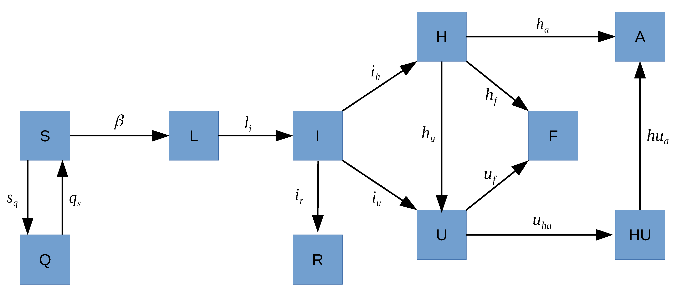
With respect to COVID-19, an individual can be considered as:
(S) susceptible, when the individual is healthy;
(Q) in lockdown, when the individual is at home to avoid the spread of the virus. In our model, lockdown only considers the March’s lockdown time;
(L) latent or exposed, when the individual has been infected but it is not infectious yet;
(I) infectious, when the individual is capable of spreading SARS-CoV-2;
(R) recovered, when the individual recovers from the disease being asymptomatic or having mild symptoms;
(H) hospitalized at ward, when the individual has severe symptoms and needs to be hospitalized;
(U) in intensive care unit (ICU), when the individual has severe symptoms and needs to be treated in the intensive care unit;
(F) deceased, when the individual dies because of the disease;
(HU) after ICU, when an individual is transferred from ICU to other non-ICU department due to improvement in the evolution but still requires hospitalization;
(A) discharged, when the individual gets better and is discharged from hospital.
We are going to use data from patients hospitalized, in ICU, discharges and deaths in the Spanish province of Granada provided by the hospital H.U. Virgen de las Nieves and we scale these data in order to generate an inclusive model that represents the whole province. The province of Granada has inhabitants, and we consider the value as constant during the simulation time. Our simulations begin on 1 March 2020 and the time step t is one day.
When the alarm state is decreed and most of the people have to be in lockdown, that is, move from
S to
Q, it is modeled by the term
, where the model parameter
determines the transit of people from
S to
Q.
takes the value 0 except for 16 March 2020 and 31 March 2020, when the lockdown and the strict lockdown began in Spain, and 700,000 and 150,000 more individuals in Granada, respectively, move from S to Q [
19].
When the lockdown finishes, the transit of individuals from Q to S is modeled by the term where the model parameter is 0 except for 13 April 2020 when the strict lockdown finishes and 150,000 individuals move from Q to S, and from 5 May to 21 June 2020, leaving the lockdown 8750 people every day due to the gradual end of the confinement.
An individual moves to latent state (L) if he/she gets infected by contact with an infectious individual. People in the hospital are isolated and controlled and, therefore, discarded for contagions. The transit is modeled by the non-linear term , where the transmission rate parameter has to be calibrated. Furthermore, this parameter will change over time due to the global public health interventions.
A latent individual transits to infectious state after a while and this is modeled by the linear term
, where the latency period
is the time from the moment in which an individual is infected until the moment in which is able to transmit the virus,
. This period is different to the typical incubation period time from infection to onset, and according to [
20], it takes from 2 to 7 days. Even though there is limited evidence about the possibility of infection one or two days before onset [
21], let us consider that
may take values from 1 to 6 days, and
.
An infectious individual may become hospitalized (H), admitted to the Intensive Care Unit (U) or recover (R), and these transits are modeled by the linear terms , and , respectively. Here, we have three possible statuses for infectious individuals. Every one takes its time and has its probability, that is, , and .
is the percentage of infected who become hospitalized and days the time it takes; is the percentage of infected people admitted directly at ICU and days the time it takes. Then, the parameters of the transition from I to H and from I to U are and , respectively.
Those infected but are not hospitalized require around
days to recover [
22]. Thus, the transition from
I to
R is governed by the parameter
.
Hospitalized people may move to ICU (U) if they get worse, may die (F) or may be discharged (A). These transits are modeled by the linear terms , and , respectively. As before, here we have three possible statuses for hospitalized individuals and each one takes its time and its probability.
is the percentage of hospitalized people who need to be admitted to ICU and days the time it takes. Hence, the people in H move to U governed by the parameter .
is the percentage of hospitalized people who die after an average of days. Then, the transition parameter from H to F is .
is the percentage of hospitalized people who are discharged after an average of days in the hospital. Hence, the transition parameter from H to A is .
People in ICU (U) may decease (F) or may get better and be transferred to other non-ICU department (HU). These transits are modeled by the linear terms and , respectively. Here we have 2 possible ways for individuals in ICU, die or get better and each one takes its time.
The transition parameter from U to F is , where is the probability to die after days (in average) if the individual is in the ICU.
The parameter that governs the transition from U to is , where days is the average time an individual needs to leave the ICU because he/she gets better.
Finally, an individual in may get better and be discharged. This transit is modeled by the linear term , where , where is the average time to be discharged after leaving ICU.
Taking into account the above description of the populations and the model parameters, the following system of difference Equation (
1) describes the transmission dynamics of COVID-19 in the province of Granada (Spain) over time.
Figure 1 shows a flow diagram of how individuals may move throughout the different states with respect to the disease. Note that the right part of
Figure 1 (H, U, F, A, HU) represents the flow of patients within hospital departments. There is no movement between infectious (I) to deceased (F) as there are no data available and, because, in Spain, most of the people who die by COVID do it in the hospital. Even though it seems that there is evidence of COVID re-infections [
23,
24], they are very few and we are not going to consider it in our model.
Since other known coronaviruses have seasonal behaviour [
25], as a hypothesis, two main periods have been considered: virulence season (September to April) and non-virulence season (May to August). This division is supported by the available data related to number of hospitalizations and deaths. Due to this, some model parameter values will vary depending on the season.
2.2. Model Calibration with Uncertainty
As we have mentioned before, we obtained hospitalization data from the Spanish province of Granada with the aim of calibrating the model parameters in such a way that the model may describe the evolution of the pandemic in this area. Known parameters values are shown in
Table 1.
Hence, the model parameters
,
,
,
,
,
,
,
,
,
,
,
,
,
and
have to be calibrated in the intervals described in
Table 2. Most of these intervals are established using the available data. The initial number of latent and infectious are also established to determine an appropriate initial condition on 1 March 2020. According to the data, on 1 March there were five people in the hospital circuit and none at ICU or recovered.
To calibrate the model, we consider four different transmission rates : (1) before the lockdown; (2) after the lockdown; once the confinement has finished, (3) non-virulence season and (4) virulence season. We also take into account that the basic reproductive number of our model is consistent with real values as t goes on, time t in days.
Our main source data (hospital’s data) collect the number of daily hospitalizations, daily people in ICU, accumulated deaths and accumulated discharges in the hospitals of the province of Granada from 1 March to 22 September 2020. These data allow us to determine intervals of where to search the model parameter values during the calibration. In order to obtain suitable numerical values of the model parameters, the 10 and 90 percentiles of the stay time in each state of the hospital circuit (H, U, F, A, HU) are obtained and settled as the calibration range where looking for the proper values of the parameters. The intervals to determine the parameter values, those given by the hospital’s data and the others, can be seen in
Table 2 under the column Calibration range.
We also use the seroprevalence study [
17,
18], which determines the percentage of accumulated infected people from the whole population. According to the prevalence study of COVID-19 in Spain, carried out between May and June 2020, the accumulated infected population in the province of Granada from the 27 April to 11 May is in the range
, the range from 18 May to 1 June is
and the range from 8 June to 22 June is
.
The model calibration with uncertainty is carried out, applying the bootstrapping technique described in [
26]. This technique mainly consists of performing a deterministic calibration using the optimization algorithm NS for PSO [
27], to find a model parameter value, in their corresponding calibration ranges in
Table 2, in such a way that the model output is as close as possible to the data of hospitalized at ward, ICU, deceases and discharges, and the model output for recovered are inside the prevalence confidence interval provided by [
17,
18]. The closeness is measured using the following fitting function:
where
measures the distance from a point to an interval,
,
,
,
,
are the model output corresponding to the number of recovered, hospitalized at ward, at ICU, discharges and deaths, respectively, at the day
t, and
,
,
,
are the data of hospitalized at ward, at ICU, discharges and deaths, respectively, at the day
t.
The first three terms of the fitting function (
2) guarantee that the model prevalence fits the data of the prevalence study [
17,
18]. The last term of (
2) guarantees that the number of hospitalized at ward, at ICU, discharges and deaths returned by the model are close to their corresponding data.
Once the model is calibrated, we calculate the difference between the model output and the data for each time instant (residuals). Then, we estimate a probability distribution of the residuals. Thus, we sample 1000 times the residuals’ probability distribution, we sum up the data generating 1000 sets of perturbed data, describing the data uncertainty. Then, the model is deterministically calibrated, using NS for PSO, for the 1000 sets of perturbed data. For all the model parameter values obtained we calculate the mean and the percentiles and ( confidence interval) describing the uncertainty of the model parameters. For the model outputs, calculating the mean and the confidence intervals for each time instant, we obtain the confidence bands of the evolution of the subpopulations over time.
2.3. Vaccination
In Spain, the vaccinations started on 27 December 2020. On 23 February 2021, 3 million doses have been administered and 1.2 million people have received the two doses [
28]. In Granada, these figures correspond to an average of 526 people vaccinated every day from the beginning of the vaccination campaign. The Spanish government expect to vaccinate
of people before the end of summer 2021 [
29]. This implies an increase by six of the number vaccinated daily.
In order to simulate the effect of the vaccine in the population of the Spanish region of Granada, a new state has to be considered in the mathematical model:
We suppose that only susceptible people are vaccinated. We assume that the vaccine protects against the most dangerous symptoms of the COVID-19 and blocks the spread of the disease. The transit from S to V is modeled by the term and the transit from V to S, it is modeled by the term . Both parameters describe the number of people who are moving from one state to other, at time t.
The system of difference equations, which includes the vaccination of the population is shown in (
3). In black, the new terms.
Not every vaccinated person acquires protection against the disease. We consider the vaccine’s effectiveness as the percentage of vaccinated people who acquire immunity. The duration effect of the vaccine is also unknown, and we will assume a permanent immunity for effective vaccinations, then
for all
t. In [
30], the authors say that the vaccine’s effectiveness is
. However, in order to take into account possible mutations that may affect the effectiveness, we will consider
vaccine effectiveness. Furthermore, the first vaccination dose provides
effectiveness [
31].
Here, we are going to perform three simulations. The simulations were carried out on 10 March 2021. In the three, we vaccinate at the current pace, with effectiveness, from 27 December 2020 until 31 March. From 1 April,
- (1)
we keep vaccinating at the same pace and no new population restrictions are applied;
- (2)
the same as (1) applying stronger restrictions from 1 to 15 April;
- (3)
the same as (2) and the vaccination pace increases to fulfill coverage the 31 August 2021.
3. Results
3.1. Calibration
For calibration with uncertainty, a bootstrapping technique [
26] is applied. Technical details can be seen in
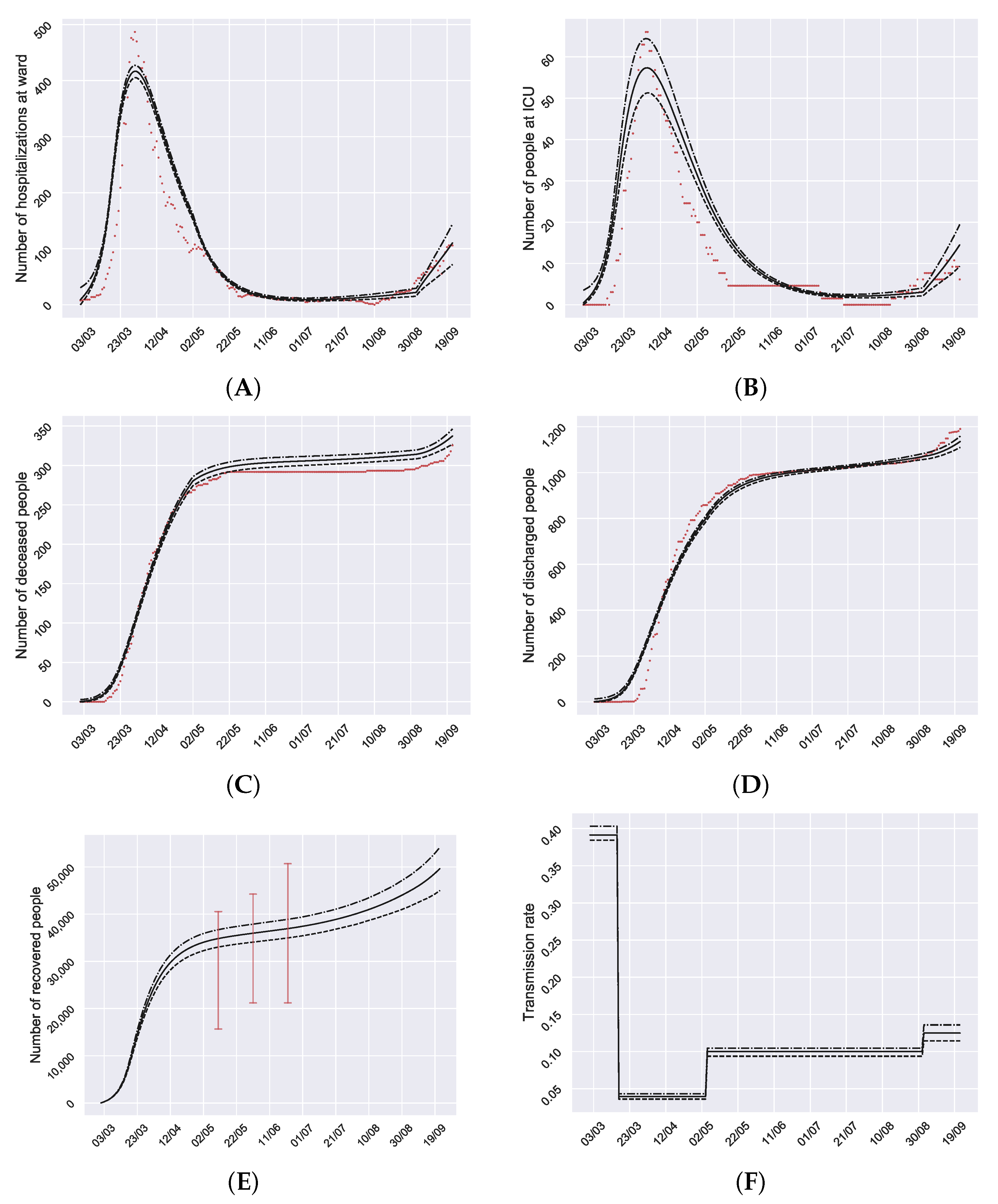
Appendix A. This way, we are able to capture and quantify the uncertainty in the evolution of the disease. The results of the calibration are good enough to represent the effects of the pandemic in Granada during the 1 March–22 September 2020 period (
Figure 2).
The mean and confidence interval of all the obtained calibrated parameters are shown in
Table 3. The availability of reliable hospital data allows us to provide realistic intervals to calibrate the model parameters and, once the model is calibrated, meaningful model parameter values describing the transitions among states of the disease.
On 1 March 2020 (initial condition) the calibrated number of infectious is 1192, CI95% 1166–1226, (
, CI95% 0.125%–0.133%) and latent 574, CI95% 559–589, (
, CI95% 0.060%–0.064%). Data provided by the hospitals in the province of Granada, from 1 March to 15 March, compared with the registry of the previous years, did not show an increase of respiratory disease cases that could be attributable to COVID-19, which is in accordance with our estimation of the low number of COVID-19 patients at the beginning of the pandemic (1 March 2020). Later, the number of infected patients experienced a great increase, which supports that the effective reproductive number
was initially very high, (
, CI95% 5.34–5.61), value which is in accordance with Sanche et al. [
32].
After the beginning of the lockdown declared by the Spanish government in 16 March, the number of infected kept growing as a consequence of the contagions produced in the previous weeks with high transmission rate
. Nevertheless, the basic reproductive number
decreased to
, CI95% 0.50–0.60, not only because of lockdown but also the social distancing, the use of face-masks and other population measures, reducing the
, as can be seen in
Figure 2F.
During the non-virulence season after the lockdown is finished, May–August, the incidence of the disease kept low, with a stabilization of the number of hospitalizations and deaths. The
value was low,
, CI95% 1.31–1.46, but it increases until slightly higher values than at the beginning of the virulence season (
, CI95% 1.59–1.89). This can be observed with the increase of hospitalized and intensive care unit people, together with the end of the stagnation in the number of deceased and discharged in September on
Figure 2 (leftmost part of the figure).
Different calibrated model parameter values can be seen in
Table 3 for virulence and non-virulence seasons. More precisely, the percentage of infected people who needed hospitalization (hospitalization at ward
, or ICU treatment
). During the virulence season, about
of the infected people needed hospitalization, and
of the infected people entered the ICU directly without passing through the hospitalization ward. During the non-virulence season, about
of the infected people need hospitalization at ward, and
of the infected people enter the ICU directly without passing through the hospitalization ward. Analogous differences can be seen in probability parameters
and
where in the non-virulence season the probability to get worse is significantly lower.
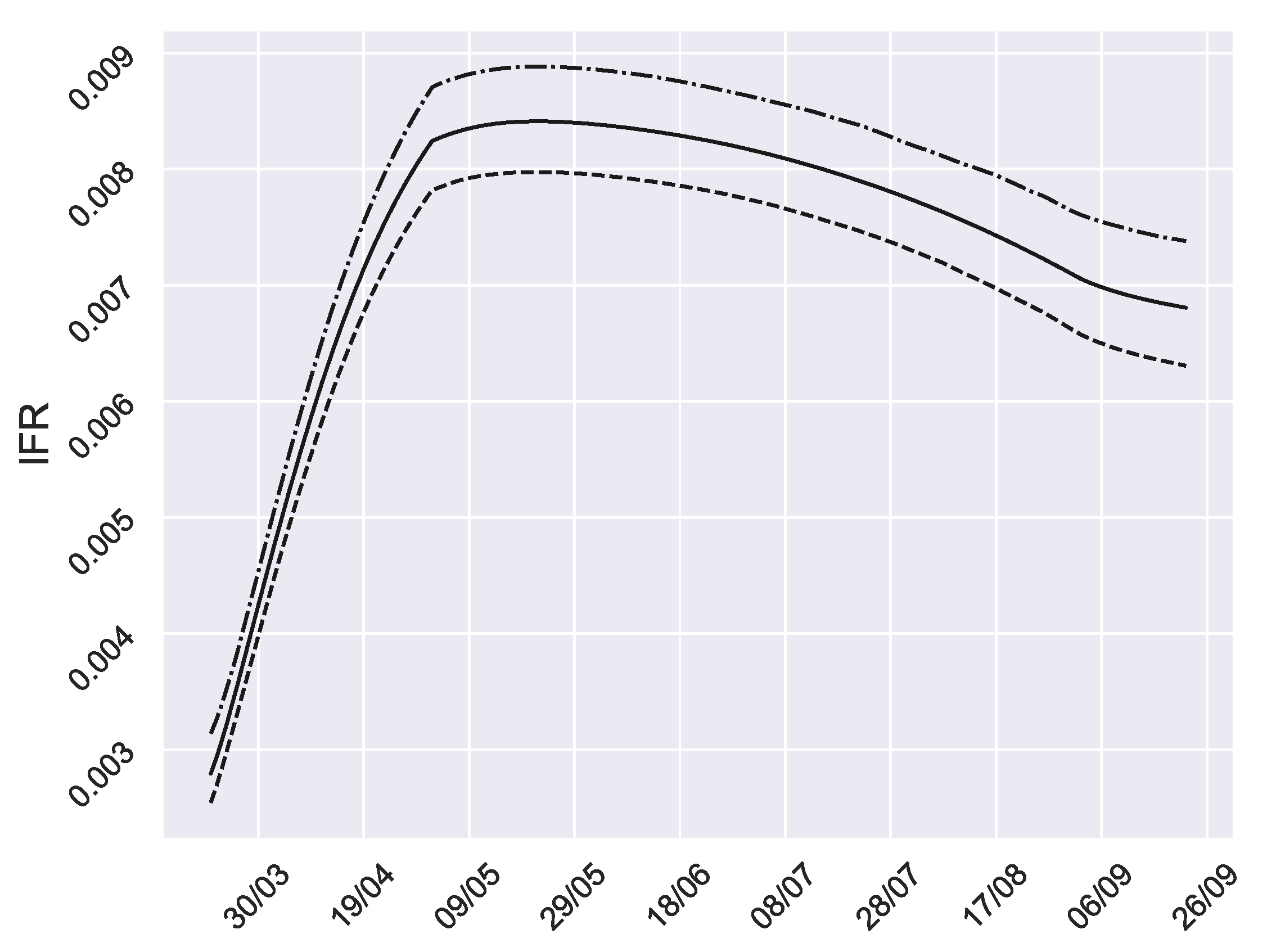
Furthermore, in
Figure 3, we can see the evolution of the infection fatality ratio (IFR), that is, the proportion of infected people who die (accumulated). This is a measure of the disease severity [
33]. After April 2020, the IFR decreased until October, corresponding to the non-virulence season.
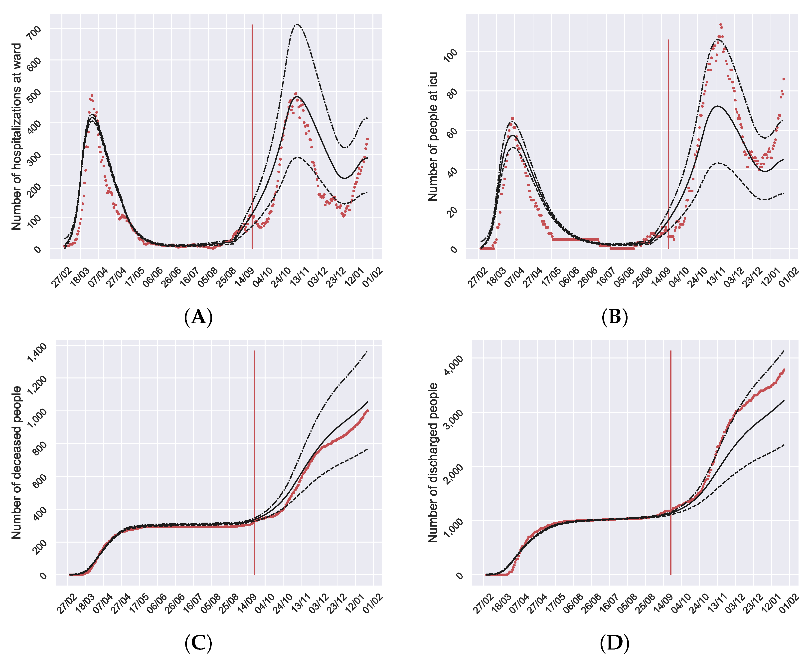
3.2. Model Validation
In order to validate the calibration of the model, data from 23 September 2020 until 26 January 2021 have been collected with the aim of comparing the error between the model evolution and the real data not used for calibration. The results can be seen in
Figure 4. The model
confidence bands capture most of the data after 23 September (red vertical line) taking into account that this is the infectious disease most intervened in history with interventions whose actual effect is unknown or contains a lot of uncertainty. In fact, the model is able to predict the evolution of the second and the beginning of the third wave.
3.3. Vaccination Simulation
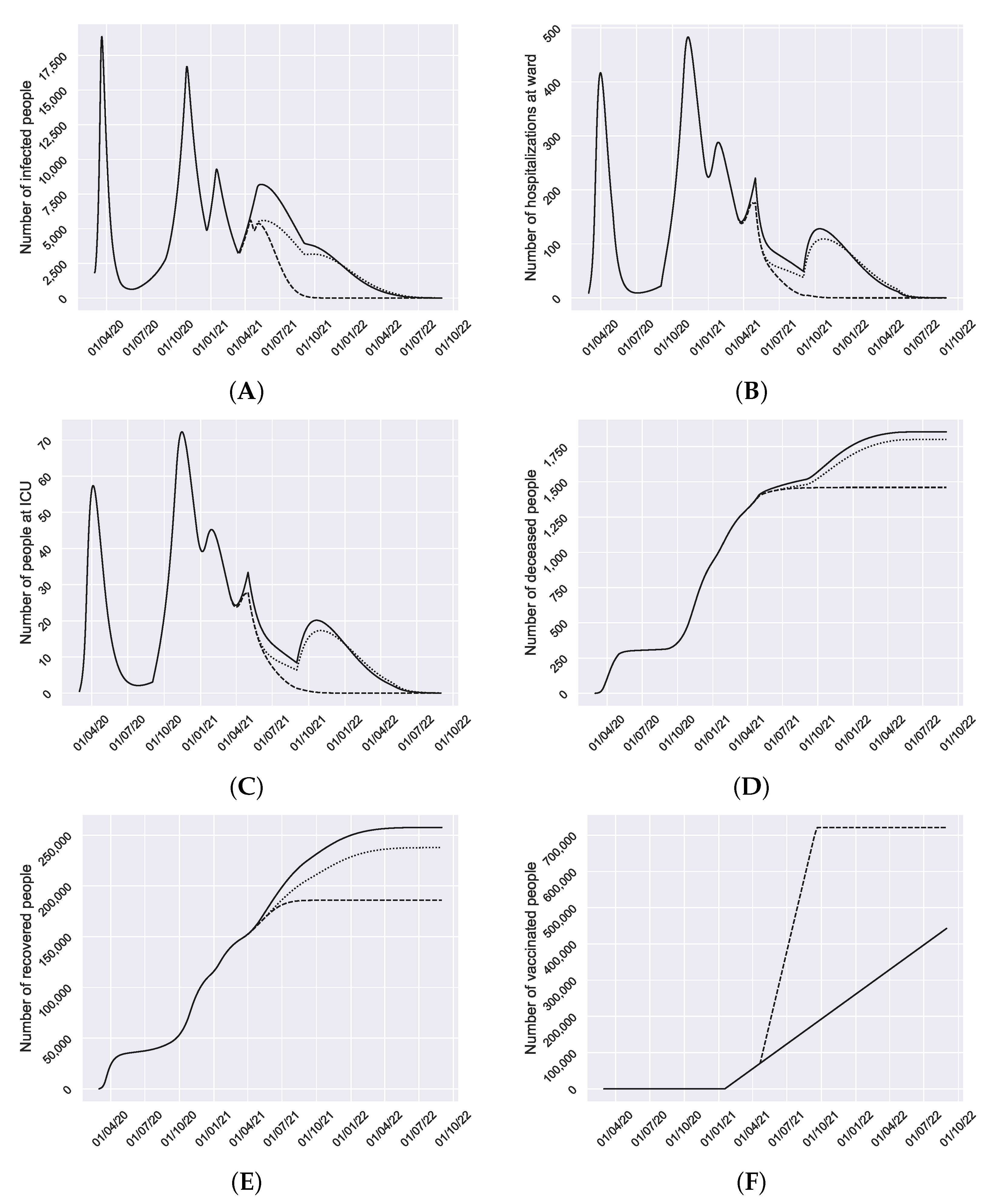
Once the model has been calibrated and validated, we can simulate with reliability possible scenarios for the future. In
Figure 5 we can see the result of the simulation scenarios: (1) the current situation does not change; (2) scenario (1) with stronger restrictions from 1–15 April; (3) scenario (2) and
of population is vaccinated at the end of Summer with an effectiveness of
.
Figure 5 shows that the 3rd wave is finishing and the 4th wave will start soon because at the beginning of March the restrictions have been relaxed. However, the peak of this 4th wave may be high if we are not careful satisfying the population measures (solid black line in
Figure 5). The application of strong restrictions again or the increase of the pace of vaccination are the strategies to avoid a new high wave (dotted and dashed lines in
Figure 5) and quickly starts to decline the number of infected. Similar effects can be seen in hospitalizations and ICU graphs. In
Figure 5D, a stabilization in the deaths can be seen around May.
As we can see, in the three cases, when next May starts, we enter the non-virulence season and the number of infected people declines. In the scenarios (1) and (2) where the vaccination pace does not increase, the decline may have new waves for hospitalized at ward and ICU next October. Although this wave is very low for infected, as we are in the virulence season, the transition parameters to subpopulations H and U are significantly higher, explaining why a very small wave in infected people produce noticeable waves in hospitalized at ward and ICU. In the scenario (3) the decline is very fast, keeping it low without new waves.
This general decline happens because the percentage of immunized people (recovered + vaccinated), appearing in the last row (% immunized) of each scenario in
Table 4, is close or greater than the percentage of immunized people required for the herd immunity, given by
, rows
H in
Table 4.
It is noticeable that in September, starting the next virulence season, the percentage of immunized people is high enough to avoid a new infected wave (see
Figure 5) if we are careful and we satisfy non-pharmaceutical measures as the use of face-masks, social distancing, etc. Especial mention deserves the scenario 3, because on 1 September the percentage of immunized people is so high that the return to normal life may be very likely.
Although these results seem to be optimistic, the social distancing, face-masks and other non-pharmaceutical measures cannot be removed suddenly. Otherwise, the transmission rate increases, also , and a new outbreak (wave) may arise when virulence season comes again, except, maybe, in scenario 3 where most of the people is immunized, mainly, because the increase of the vaccinated pace.
The simulations shown in
Figure 5 may help policy makers in hospitals and public health to plan the use and distribution of resources to face the coming months.
4. Discussion
Explanatory mathematical models of infectious diseases are intended to allow to predict the evolution of the disease considering a wide range of possible scenarios. They should be able to estimate the healthcare demands that will have to be covered by hospitals early enough as to implement management and operative adaptations regarding multiple aspects, including the extension of ICU to other places that could be equipped and be used for the management of the COVID-19 patients, as well as the reservation of out-of-hospital stays, such as hotels, for health personnel or even for patients with low severity who must be lockdown in a controlled environment [
34].
In this paper we propose a mathematical model to study the current transmission dynamics of SARS-CoV-2. It is a SEIR model where the circuit of patients moving inside the hospital dependencies, the particular features of the disease and the asymptomatic infectious, a principal source of contagiousness [
35], are considered, returning a more precise portrait of the use of hospital resources, taking into account the uncertainty of the phenomenon and the data. We tested the model using registered cases and population data from the hospitals of the Spanish province of Granada that represent a size of near 1 million citizens. In this province, there is low density of population and there was a low prevalence of COVID-19 on the spring 2020 outbreak. The model is able to predict the third and the fourth wave of the pandemic.
A direct and permanent line of communication is important for the transmission of data in real time between the heads of hospital centres and the teams in charge of analysing the epidemiological evolution of the disease, especially through tools such as the one presented in this paper. This will ensure the optimization of future predictions on the basis of the augmentation of the knowledge database, contributing to face the fluctuations that may appear in the transmission of the virus depending on variables that are not sufficiently clarified at the moment.
One of the strong aspects of our model is that it is possible to calibrate and validate from data collected and reported through an informative protocol agreed at the province of Granada, which ensures homogeneity as well as prevents biases that may appear on the count of each type of subject, consideration of infected by diagnostic, etc. Also, the model has been fed regularly with new data to update the predictions.
Good planning supported by models like the one we propose permits better distribution of the hospital resources, preparing a COVID-19 area without reducing the care attention to patients with other diseases, preventing the collapse of the health services, as happened last March-April 2020 and January-February 2021.
Our simulations show that we have to keep population measures and/or increase the vaccination pace in order to control the pandemic and avoid new concerning outbreaks. However, a decline in the number of infectious is expected to start in May without a new increase in September when the virulence season arrives if we are able to maintain population non-pharmaceutical measures as the use of face-masks, social distancing, etc.
The transmission capacity of the virus at the beginning of the pandemic was very high, with
greater than 5. Numerous studies have stated the effectiveness of non-pharmaceutical measures in reducing the transmission of respiratory virus [
36,
37,
38,
39,
40,
41,
42,
43,
44,
45]. Then,
decreased significantly, reaching an average of
and making it possible to control the pandemic by approaching to 1. The return to normal life as it was before the pandemics, is not to be expected in the short term, because our simulations assume low transmission rates due to the social distancing, face-masks, restricted schedules, curfew and other non-pharmaceutical measures. However, we expect these non-pharmaceutical measures will be relaxed as the immunized people increases. Nevertheless, if the rate of vaccination grows sufficiently, it is possible that the return to normal life becomes very likely.
5. Conclusions
Mathematical models allow us to make predictions that may provide enough time for the health systems to establish the appropriate measures to face outbreaks that could collapse human and material resources. Moreover, future pharmaceutical and non-pharmaceutical interventions, as well as aspects related to SARS-CoV-2 biology and behaviour, can be represented through the model parameters to act as modulator of the transmission rate what provide the required flexibility to adapt the model throughout the time.
The modified SEIR model presented in this paper can be a useful tool for providing insight into the transmission dynamics of SARS-CoV-2. It considers the circuit of patients moving inside the hospital dependencies, returning a more precise portrait of the use of hospital resources to foresee future needs.
Once the model is calibrated and validated, three scenarios are simulated to evaluate the evolution of COVID-19 in Granada. The simulations show that we are finishing the 3rd wave but the 4th wave is around the corner reaching the peak in May 2021. In the worst case, the 4th wave seems to be a bit lower than the previous ones.
In any case, a decline in the number of infected people is expected in all the simulated scenarios, starting in May and maintained when we change to the virulence season next September. This is possible if we keep lower transmission rates, and consequently low , due to the social distancing and other non-pharmaceutical measures. That is, we will not be out of danger yet. Nevertheless, we will be able to resume the life as we knew it before the pandemic relaxing measures of social situation and face-masks in a gradual and controlled way to avoid new outbreaks as the percentage of immunized people increases.
Limitations of the Model
The proposed model is a classical system of difference equations. For its building, we assume usual hypotheses as the homogeneous mixing of the population (any individual may infect any individual). No age groups are considered, and the hospitalization and decease rate may vary depending on the age of the individuals. Also, we assume that all lockdown people are susceptible, when latent, asymptomatic infectious and recovered may also be in lockdown. Furthermore, mobility and other spatial aspects are not considered.
Furthermore, we assume that there is no re-infection or is not significant and the vaccine blocks the transmission of COVID-19. Furthermore, we assume a permanent protection for those who the vaccine is effective. If these hypotheses were eventually not true, an increase in the number of cases could be seen next autumn.
Transitions from infected (I) or latent (L) to quarantine (Q) may be included in the model as infected individuals that are quarantined after tested positive or via contact tracing. However, it turns the model more complex as mentioned in [
46,
47] where the authors say that in a standard ODE, to incorporate additional heterogeneities, as household structure, requires a considerable degree of model complexity and large computational expense. And, also, the transitions should be fed with data, not always available.
It is clear that the tests are being an important tool with the aim at controlling the pandemics and quarantining the positive people. However, when a person is tested and the test is positive, he/she may have been previously a period of time (unknown) infecting others and it may reduce the global transmission rate. However, a high percentage of the infections are due to the asymptomatic infected people, which percentage is still unknown but it seems to be high (“the proportion of symptomatic cases is low, ranging from 13 to 18%” [
48]) and their control may be reduced.
The not consideration of the above details in the model and others, may increase a bit the transmission rate beta respect the real one and it may affect the estimation or and the periods where herd immunity is reached will be a bit later.
It is important to consider that the model must be particularized for each population, either provincial or larger, since the transmission rate must respond to the effect of health policy measures and the response of the population to the recommendations, such as opening educational centers, social distancing, use of face-masks, adaptation of public and private services to establish physical barriers that hinder the spread of the virus, etc.
Author Contributions
Data retrieval and curation, COVID_19 Granada Study Group; Conceptualization; J.M.G. and F.R.-S.; Modeling, J.M.G., D.M.-R., F.R.-S., S.-M.S., R.-J.V.; Methodology, D.M.-R., S.-M.S. and R.-J.V.; Software, D.M.-R.; validation, J.M.G., F.R.-S.; writing, J.M.G., D.M.-R., R.-J.V. All authors have read and agreed to the published version of the manuscript.
Funding
This research was funded by the Spanish Ministerio de Economía, Industria y Competitividad (MINECO), the Agencia Estatal de Investigación (AEI) and Fondo Europeo de Desarrollo Regional (FEDER UE) grant MTM2017-89664-P and the European Union through the Operational Program of the [European Regional Development Fund (ERDF)/European Social Fund (ESF)] of the Valencian Community 2014–2020. Files: GJIDI/2018/A/010 and GJIDI/2018/A/009 and the Ramón Areces Foundation, Madrid, Spain (CIVP18A3920).
Institutional Review Board Statement
The study has been accepted by the ethical committee of the Regional Government of Andalusia. The acceptance document may be available on request.
Informed Consent Statement
Patient consent was waived due to the fact that this study only involves anonymized data of the number of patients being admitted at the hospital. This study had not access to data of any particular patient.
Data Availability Statement
Data from hospitals may be available on request. Prevalence data can be obtained from [
17,
18].
Acknowledgments
We acknowledge COVID-19_Granada Study Group, composed by José Manuel Garrido Jiménez, Antonio Cansino Osuna, Juan Carlos Carrillo Santos, Cristina Carvajal Pedrosa, Mª Angeles García Rescalvo, Francisco José Guerrero García, Sebastián Manzanares Galán, Francisco Marti Jiménez, Manuel Enrique Reyes Nadal, Pedro Manuel Ruiz Lorenzo, José Luis Salcedo Lagullón, Indalecio Sánchez-Montesinos García, Fernando Rodríguez-Serrano, for data retrieval and curation.
Conflicts of Interest
The authors declare no conflict of interest.
Appendix A
Taking into account the general procedure presented in [
26], we study error terms for the estimated parameters and resample these error terms using bootstrapping. Then, we obtain new data by adding the resampled error to the output model. For each new data, we estimate the parameters.
This is based on the bootstrapping method, more specifically in residual bootstrapping, which is a commonly used and robust method, that can deal fitly dynamical systems, which in turn often violate the standard assumptions for residuals of traditional methods such as normality, independence, homoscedasticity and not autocorrelation.
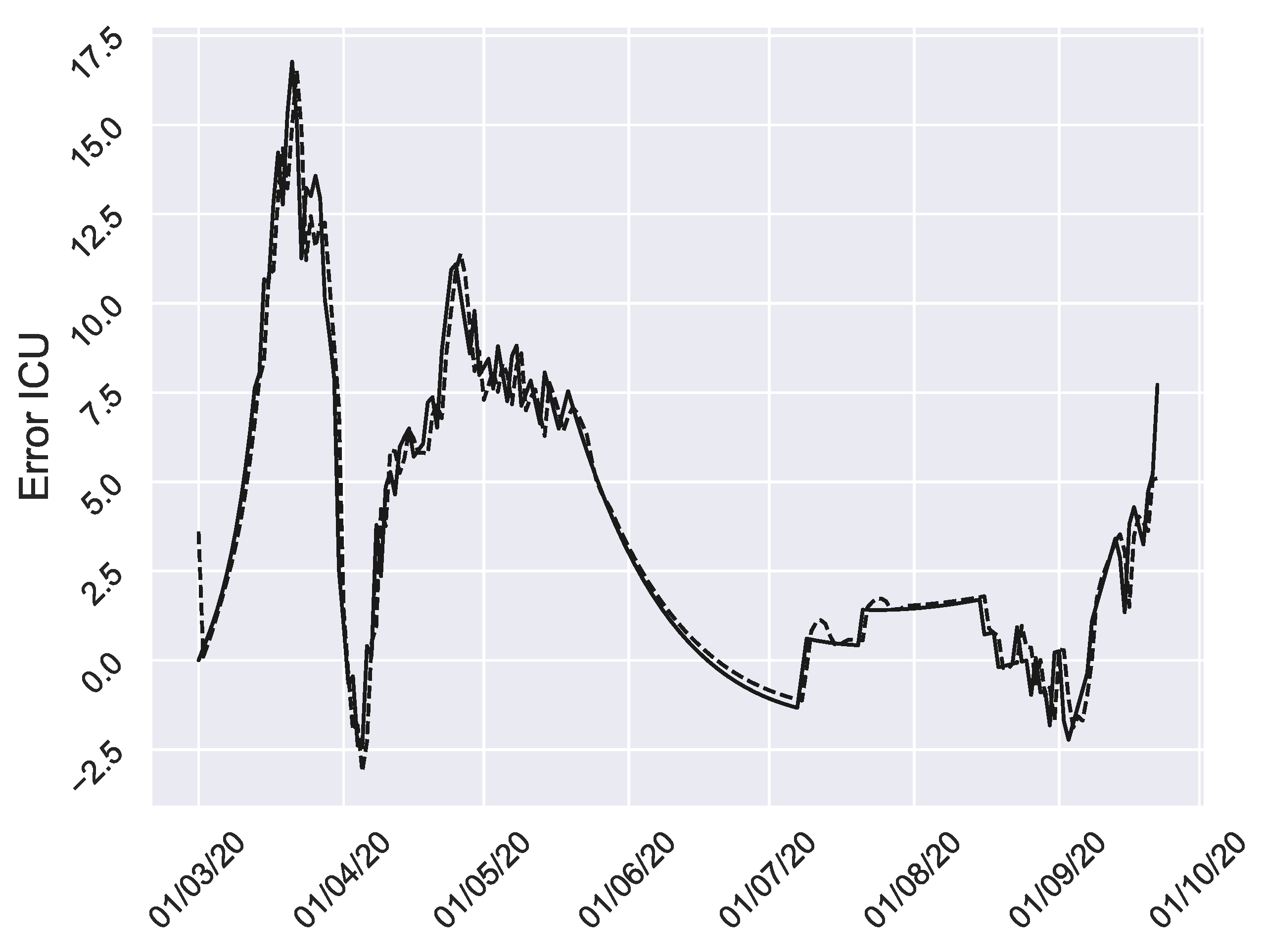
To do this, we implement the following steps. First we calibrate the model to the data, thus obtaining a first estimate of the parameters. Then, residuals are obtained from the difference of the outputs of the model fitted to the data and the real ones. In
Figure A1 we can see the residuals for ICU (solid line).
Now, we apply the Pearson correlation coefficient in order to analyze the correlation between the error terms. The results appear in
Table A1. We reject the null hypothesis if the p-value is less than
.
Table A1.
Pearson correlation coefficient and the corresponding p-values.
Table A1.
Pearson correlation coefficient and the corresponding p-values.
| | Coefficient | p-Value | | Coefficient | p-Value |
|---|
| 0.693 | 0 | | 0.019 | 0.782 |
| −0.213 | 0.00215 | | −0.122 | 0.08 |
| −0.115 | 0.00769 | | 0.3164 | 0 |
We would like to comment about the correlation coefficient
in
Table A1. It denotes a moderate correlation, however, in order to simplify the analysis and assuming the corresponding errors, we are going to ignore this moderate correlation.
In the next step, we check the assumptions for residuals of asymptotic methods by computing a hypothesis test, where the purpose of it is whether the autocorrelation values are significantly different from zero or not. In other words, this non-parametric test is used to check the hypothesis that the elements of a sequence are mutually independent. For that, we figure out the autocorrelation function values and their variances in the residual terms for different lags
k, according to the formulas in [
26]. In all the cases (people hospitalized at ward, people at ICU, discharged people and deceased people) there is significant autocorrelation for lags
,
,
and
, respectively.
Accordingly, the auto-dependency of residuals can be described using autoregressive model (AR) for each residual term. Hence, we can estimate the underlying white noise by subtracting the autocorrelation from the errors. In
Figure A1 (dashed line) we can see the AR for ICU.
Figure A1.
Residuals of ICU. Solid line are the actual residuals and the dashed line is the AR approximation.
Figure A1.
Residuals of ICU. Solid line are the actual residuals and the dashed line is the AR approximation.
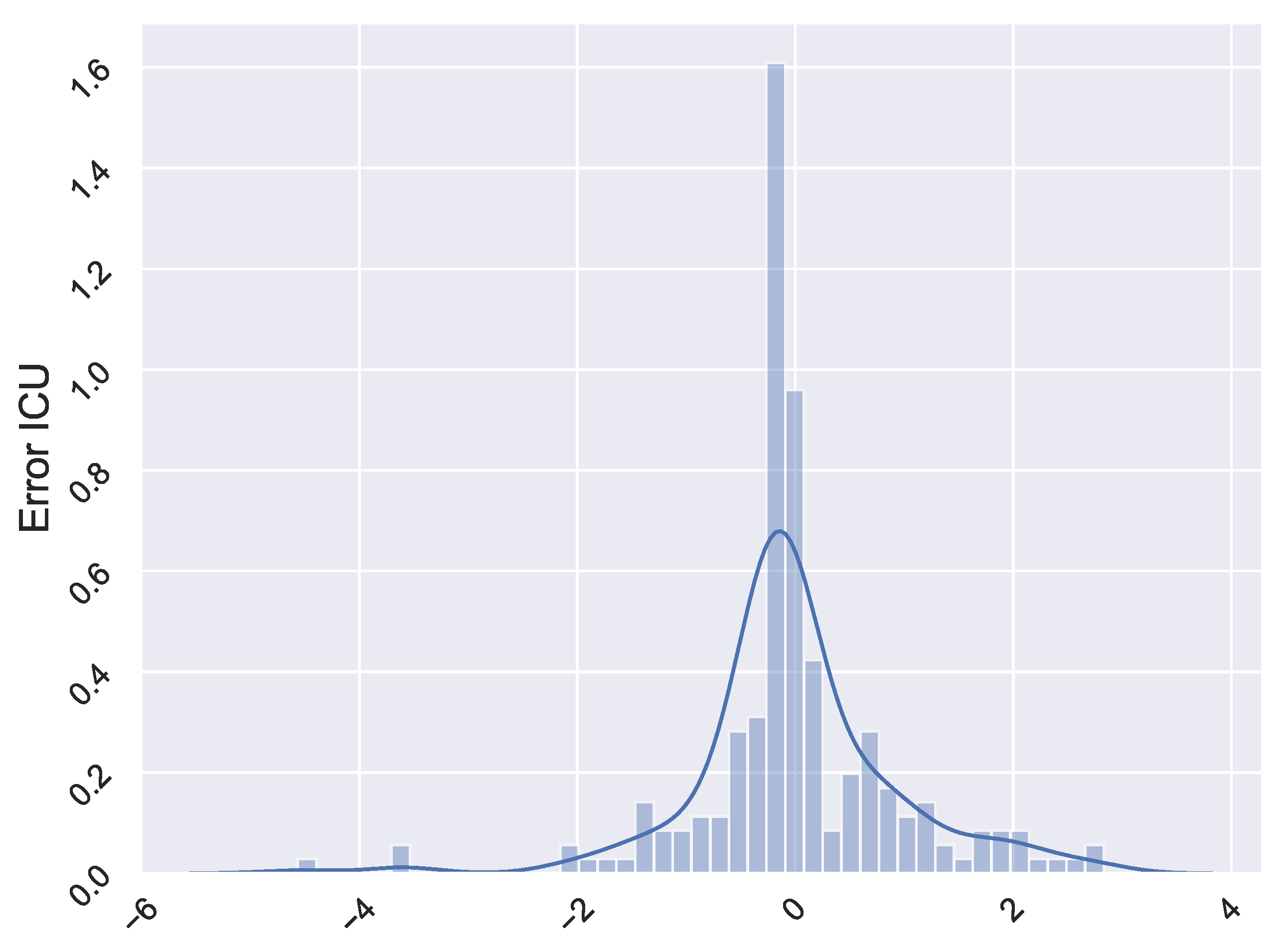
In the following step, we assess the independence of the underlying white noise by autocorrelation and normality test. With regard to the former, we implement the same procedure as before and the test statistic is not significant for all lags in the four cases. This means that there is no significant autocorrelation in the underlying noise, that is, independence. Regarding the normality test, Kolmogorov-Smirnov test is used to make a determination as to whether the distribution of underlying white noise matches the characteristics of a normal distribution. In all cases, the underlying error terms are not normally distributed. This fact is reflected in the
Figure A2.
In the next step we resample this white noise using a nonparametric bootstrapping, since it is not normally distributed, to obtain new residual values for each time instant. In this technique, each new set of residuals is generated by resampling randomly, with replacement, from the original white noise dataset. In total, we use 1000 bootstraps. These sets are added to the data, thereby creating 1000 new data sets. Then, new model parameter values are obtained by calibrating the model to each one of the 1000 new data sets. At the end of the process, we have 1000 estimates for the parameters, which can be used to construct the empirical distribution.
Figure A2.
White noise histogram of AR model for ICU residual terms.
Figure A2.
White noise histogram of AR model for ICU residual terms.
References
- Zhang, T.; Wu, Q.; Zhang, Z. Probable Pangolin Origin of SARS-CoV-2 Associated with the COVID-19 Outbreak. Curr. Biol. 2020, 30, 1346–1351.e2. [Google Scholar] [CrossRef] [PubMed]
- Zhou, F.; Yu, T.; Du, R.; Fan, G.; Liu, Y.; Liu, Z.; Xiang, J.; Wang, Y.; Song, B.; Gu, X.; et al. Clinical course and risk factors for mortality of adult inpatients with COVID-19 in Wuhan, China: A retrospective cohort study. Lancet 2020, 395, 1054–1062. [Google Scholar] [CrossRef]
- Barmparis, G.D.; Tsironis, G. Estimating the infection horizon of COVID-19 in eight countries with a data-driven approach. Chaos Solitons Fractals 2020, 135, 109842. [Google Scholar] [CrossRef] [PubMed]
- Gatto, M.; Bertuzzo, E.; Mari, L.; Miccoli, S.; Carraro, L.; Casagrandi, R.; Rinaldo, A. Spread and dynamics of the COVID-19 epidemic in Italy: Effects of emergency containment measures. Proc. Natl. Acad. Sci. USA 2020, 117, 10484–10491. [Google Scholar] [CrossRef] [Green Version]
- Tang, B.; Wang, X.; Li, Q.; Bragazzi, N.L.; Tang, S.; Xiao, Y.; Wu, J. Estimation of the Transmission Risk of the 2019-nCoV and Its Implication for Public Health Interventions. J. Clin. Med. 2020, 9, 462. [Google Scholar] [CrossRef] [Green Version]
- Liu, Z.; Magal, P.; Seydi, O.; Webb, G. A COVID-19 epidemic model with latency period. Infect. Dis. Model. 2020, 5, 323–337. [Google Scholar] [CrossRef]
- Prem, K.; Liu, Y.; Russell, T.W.; Kucharski, A.J.; Eggo, R.M.; Davies, N.; Jit, M.; Klepac, P.; Flasche, S.; Clifford, S.; et al. The effect of control strategies to reduce social mixing on outcomes of the COVID-19 epidemic in Wuhan, China: A modelling study. Lancet Public Health 2020, 5, e261–e270. [Google Scholar] [CrossRef] [Green Version]
- Grauer, J.; Löwen, H.; Liebchen, B. Strategic spatiotemporal vaccine distribution increases the survival rate in an infectious disease like Covid-19. Sci. Rep. 2020, 10, 1–10. [Google Scholar] [CrossRef] [PubMed]
- Hou, C.; Chen, J.; Zhou, Y.; Hua, L.; Yuan, J.; He, S.; Guo, Y.; Zhang, S.; Jia, Q.; Zhao, C.; et al. The effectiveness of quarantine of Wuhan city against the Corona Virus Disease 2019 (COVID-19): A well-mixed SEIR model analysis. J. Med. Virol. 2020, 92, 841–848. [Google Scholar] [CrossRef] [Green Version]
- Serhani, M.; Labbardi, H. Mathematical modeling of COVID-19 spreading with asymptomatic infected and interacting peoples. J. Appl. Math. Comput. 2020. [Google Scholar] [CrossRef]
- Avila-Ponce de León, U.; Pérez, A.G.; Avila-Vales, E. An SEIARD epidemic model for COVID-19 in Mexico: Mathematical analysis and state-level forecast. Chaos Solitons Fractals 2020, 140, 110165. [Google Scholar] [CrossRef]
- Sarkar, K.; Khajanchi, S.; Nieto, J.J. Modeling and forecasting the COVID-19 pandemic in India. Chaos Solitons Fractals 2020, 139, 110049. [Google Scholar] [CrossRef] [PubMed]
- Giordano, G.; Blanchini, F.; Bruno, R.; Colaneri, P.; Filippo, A.D.; Matteo, A.D.; Colaneri, M. Modelling the COVID-19 epidemic and implementation of population-wide interventions in Italy. Nat. Med. 2020, 26, 855–860. [Google Scholar] [CrossRef]
- Brauer, F.; Castillo-Chavez, C. Mathematical Models in Population Biology and Epidemiology; Springer: New York, NY, USA, 2012. [Google Scholar] [CrossRef]
- Shim, E.; Tariq, A.; Choi, W.; Lee, Y.; Chowell, G. Transmission potential and severity of COVID-19 in South Korea. Int. J. Infect. Dis. 2020, 93, 339–344. [Google Scholar] [CrossRef] [PubMed]
- Instituto de Estadistica y Cartografia de Andalucia. Available online: http://www.juntadeandalucia.es/institutodeestadisticaycartografia (accessed on 11 March 2021).
- Pollán, M.; Pérez-Gómez, B.; Pastor-Barriuso, R.; Oteo, J.; Hernán, M.A.; Pérez-Olmeda, M.; Sanmartín, J.L.; Fernández-García, A.; Cruz, I.; de Larrea, N.F.; et al. Prevalence of SARS-CoV-2 in Spain (ENE-COVID): A nationwide, population-based seroepidemiological study. Lancet 2020, 396, 535–544. [Google Scholar] [CrossRef]
- Informe Final del Estudio Nacional de Sero-Epidemiología de la Infección por SARS-COV-2 en España (Sero-Epidemiology National Study of the Infection for SARS-COV-2 in Spain. Final Report (in Spanish)). Available online: https://www.mscbs.gob.es/ciudadanos/ene-covid/docs/ESTUDIO_ENE-COVID19_INFORME_FINAL.pdf (accessed on 6 July 2020).
- Google. Google Local Mobility Reports about COVID-19. Available online: https://www.google.com/covid19/mobility/ (accessed on 11 March 2021).
- Guan, W.J.; Ni, Z.Y.; Hu, Y.; Liang, W.H.; Ou, C.Q.; He, J.X.; Liu, L.; Shan, H.; Lei, C.L.; Hui, D.S.; et al. Clinical Characteristics of Coronavirus Disease 2019 in China. N. Engl. J. Med. 2020, 382, 1708–1720. [Google Scholar] [CrossRef] [PubMed]
- Anderson, R.M.; Heesterbeek, H.; Klinkenberg, D.; Hollingsworth, T.D. How will country-based mitigation measures influence the course of the COVID-19 epidemic? Lancet 2020, 395, 931–934. [Google Scholar] [CrossRef]
- World Health Organization (WHO). Q&A on Coronaviruses (COVID-19). Available online: https://www.who.int/emergencies/diseases/novel-coronavirus-2019/question-and-answers-hub/q-a-detail/q-a-coronaviruses (accessed on 11 March 2021).
- Iwasaki, A. What reinfections mean for COVID-19. Lancet Infect. Dis. 2021, 21, 3–5. [Google Scholar] [CrossRef]
- Centers for Disease Control and Prevention. Reinfection with COVID-19. Available online: https://www.cdc.gov/coronavirus/2019-ncov/your-health/reinfection.html (accessed on 11 March 2021).
- Edridge, A.W.D.; Kaczorowska, J.; Hoste, A.C.R.; Bakker, M.; Klein, M.; Loens, K.; Jebbink, M.F.; Matser, A.; Kinsella, C.M.; Rueda, P.; et al. Seasonal coronavirus protective immunity is short-lasting. Nat. Med. 2020. [Google Scholar] [CrossRef] [PubMed]
- Dogan, G. Bootstrapping for confidence interval estimation and hypothesis testing for parameters of system dynamics models. Syst. Dyn. Rev. 2007, 23, 415–436. [Google Scholar] [CrossRef]
- Martínez-Rodríguez, D.; Colmenar, J.M.; Hidalgo, J.I.; Villanueva Micó, R.J.; Salcedo-Sanz, S. Particle swarm grammatical evolution for energy demand estimation. Energy Sci. Eng. 2020, 8, 1068–1079. [Google Scholar] [CrossRef]
- Ministerio de Sanidad. Telegram. COVID-19 Vaccination in Spain. Available online: https://t.me/sanidadgob/1047 (accessed on 23 February 2021).
- El País. The Pace Expected by the Health Ministry: A Million Vaccinated per Week. Available online: https://elpais.com/sociedad/2021-01-07/el-ritmo-que-preve-sanidad-un-millon-de-vacunados-por-semana.html (accessed on 8 January 2021).
- Polack, F.P.; Thomas, S.J.; Kitchin, N.; Absalon, J.; Gurtman, A.; Lockhart, S.; Perez, J.L.; Marc, G.P.; Moreira, E.D.; Zerbini, C.; et al. Safety and Efficacy of the BNT162b2 mRNA Covid-19 Vaccine. N. Engl. J. Med. 2020, 383, 2603–2615. [Google Scholar] [CrossRef]
- Mallapaty, S. Are COVID vaccination programmes working? Scientists seek first clues. Nature 2021, 589, 504–505. [Google Scholar] [CrossRef] [PubMed]
- Sanche, S.; Lin, Y.T.; Xu, C.; Romero-Severson, E.; Hengartner, N.; Ke, R. High Contagiousness and Rapid Spread of Severe Acute Respiratory Syndrome Coronavirus 2. Emerg. Infect. Dis. 2020, 26. [Google Scholar] [CrossRef] [PubMed]
- Centers for Disease Control and Prevention. COVID-19 Pandemic Planning Scenarios. Available online: https://www.cdc.gov/coronavirus/2019-ncov/hcp/planning-scenarios.html (accessed on 11 March 2021).
- Weissman, G.E.; Crane-Droesch, A.; Chivers, C.; Luong, T.; Hanish, A.; Levy, M.Z.; Lubken, J.; Becker, M.; Draugelis, M.E.; Anesi, G.L.; et al. Locally Informed Simulation to Predict Hospital Capacity Needs During the COVID-19 Pandemic. Ann. Intern. Med. 2020, 173, 21–28. [Google Scholar] [CrossRef] [Green Version]
- Bai, Y.; Yao, L.; Wei, T.; Tian, F.; Jin, D.Y.; Chen, L.; Wang, M. Presumed Asymptomatic Carrier Transmission of COVID-19. JAMA 2020, 323, 1406–1407. [Google Scholar] [CrossRef] [Green Version]
- Chen, S.C.; Liao, C.M. Modelling control measures to reduce the impact of pandemic influenza among schoolchildren. Epidemiol. Infect. 2007, 136, 1035–1045. [Google Scholar] [CrossRef]
- Cui, J.; Zhang, Y.; Feng, Z.; Guo, S.; Zhang, Y. Influence of asymptomatic infections for the effectiveness of facemasks during pandemic influenza. Math. Biosci. Eng. 2019, 16, 3936. [Google Scholar] [CrossRef]
- Chen, S.C.; Liao, C.M. Cost-effectiveness of influenza control measures: A dynamic transmission model-based analysis. Epidemiol. Infect. 2013, 141, 2581–2594. [Google Scholar] [CrossRef]
- Arinaminpathy, N.; Raphaely, N.; Saldana, L.; Hodgekiss, C.; Dandridge, J.; Knox, K.; McCaarthy, N.D. Transmission and control in an institutional pandemic influenza A(H1N1) 2009 outbreak. Epidemiol. Infect. 2011, 140, 1102–1110. [Google Scholar] [CrossRef] [Green Version]
- Cowling, B.J.; Ali, S.T.; Ng, T.W.Y.; Tsang, T.K.; Li, J.C.M.; Fong, M.W.; Liao, Q.; Kwan, M.Y.; Lee, S.L.; Chiu, S.S.; et al. Impact assessment of non-pharmaceutical interventions against coronavirus disease 2019 and influenza in Hong Kong: An observational study. Lancet Public Health 2020, 5, e279–e288. [Google Scholar] [CrossRef]
- Tracht, S.M.; Del Valle, S.Y.; Hyman, J.M. Mathematical Modeling of the Effectiveness of Facemasks in Reducing the Spread of Novel Influenza A (H1N1). PLoS ONE 2010, 5, e9018. [Google Scholar] [CrossRef]
- Aiello, A.E.; Murray, G.F.; Perez, V.; Coulborn, R.M.; Davis, B.M.; Uddin, M.; Shay, D.K.; Waterman, S.H.; Monto, A.S. Mask use, hand hygiene, and seasonal influenza-like illness among young adults: A randomized intervention trial. J. Infect. Dis. 2010, 201, 491–498. [Google Scholar] [CrossRef] [PubMed] [Green Version]
- Lee, S.A.; Grinshpun, S.A.; Reponen, T. Respiratory Performance Offered by N95 Respirators and Surgical Masks: Human Subject Evaluation with NaCl Aerosol Representing Bacterial and Viral Particle Size Range. Ann. Occup. Hyg. 2008, 52, 177–185. [Google Scholar] [CrossRef] [PubMed] [Green Version]
- Brienen, N.C.J.; Timen, A.; Wallinga, J.; Van Steenbergen, J.E.; Teunis, P.F.M. The Effect of Mask Use on the Spread of Influenza During a Pandemic. Risk Anal. 2010, 30, 1210–1218. [Google Scholar] [CrossRef] [PubMed]
- Sim, S.; Moey, K.; Tan, N. The use of facemasks to prevent respiratory infection: A literature review in the context of the Health Belief Model. Singap. Med. J. 2014, 55. [Google Scholar] [CrossRef] [Green Version]
- House, T.; Keeling, M.J. Deterministic epidemic models with explicit household structure. Math. Biosci. 2008, 213, 29–39. [Google Scholar] [CrossRef] [PubMed]
- Hilton, J.; Keeling, M.J. Incorporating household structure and demography into models of endemic disease. J. R. Soc. Interface 2019, 16, 20190317. [Google Scholar] [CrossRef] [Green Version]
- Subramanian, R.; He, Q.; Pascual, M. Quantifying asymptomatic infection and transmission of COVID-19 in New York City using observed cases, serology, and testing capacity. Proc. Natl. Acad. Sci. USA 2021, 118, e2019716118. [Google Scholar] [CrossRef]
| Publisher’s Note: MDPI stays neutral with regard to jurisdictional claims in published maps and institutional affiliations. |
© 2021 by the authors. Licensee MDPI, Basel, Switzerland. This article is an open access article distributed under the terms and conditions of the Creative Commons Attribution (CC BY) license (https://creativecommons.org/licenses/by/4.0/).


 ,
, 


