An Operator-Based Scheme for the Numerical Integration of FDEs

Abstract

An operator-based scheme for the numerical integration of fractional differential equations is presented in this paper. The generalized differential operator is used to construct the analytic solution to the corresponding characteristic ordinary differential equation in the form of an infinite power series. The approximate numerical solution is constructed by truncating the power series, and by changing the point of the expansion. The developed adaptive integration step selection strategy is based on the controlled error of approximation induced by the truncation. Computational experiments are used to demonstrate the efficacy of the proposed scheme.

1. Introduction

Fractional differential equations (FDEs) play an important role in many research fields. From classical applications of FDEs in modeling viscoelasticity [1,2], to engineering problems [3,4], to more novel fields for the subject such as medical research [5,6] and economics [7,8], FDEs are becoming increasingly widespread. It is natural that a wider usage of fractional-order models has led to a growing interest in numerical integration of FDEs. Some examples of recent research are given below.

A numerical integration technique based on converting the FDE into a set consisting of integral and algebraic equations is presented in [9]. A recursive algorithm based on the Laplace decomposition is used to construct semi-analytical solutions to a Ray-tracing equation in [10]. A new scheme for the construction of numerical solutions that can be applied to several types of fractional derivatives is discussed in [11]. The Ritz approximation is applied to construct numerical solutions to the fractional Fokker–Planck equation in [12]. An approach based on Chebyshev polynomials with time-dependent coefficients is employed to construct numerical solutions to Caputo-type time–space fractional partial differential equations with variable coefficients in [13].

Müntz polynomials are used in conjunction with the collocation to develop a scheme for the numerical integration of FDEs in [14]. Chebyshev polynomials are used in a similar scheme in [15]. The infinite state representation of the Caputo derivative is used in [16] to develop an algorithm for the numerical integration of FDEs. A number of approaches applying wavelets to obtain numerical solutions to FDEs have been considered in [17,18]. A survey of current methods and a collection of software for the integration of FDEs, including explicit, implicit and predictor–corrector methods can be found in [19].

The main objective of this paper is to present a novel FDE integration scheme based on the generalized differential operator technique. The presented technique consists of constructing piecewise-polynomial approximations to the solutions of FDEs via power series. Using these approximations, integration with an adaptive step-size is performed to construct the numerical solution.

Riccati-type equations have recently been discussed in a number of publications concerned with presenting novel FDE integration schemes. He’s variational method is applied to the fractional Riccati equation in [20]. A novel homotopy perturbation technique is applied to fractional Riccati models in [21]. A modification of the homotopy perturbation method is used in [22] to construct numerical solutions to the Riccati-type FDEs.

As an example, the following form of the fractional Riccati equation is considered in developing the numerical FDE integration strategy:

$$x{\left({}^C{\mathrm{D}}^{1/2}\right)}^{2}y=a_0+a_{1}y+a_2{y}^2;a_0,a_1,a_2\in \mathbb{R},$$

(1)

where ${}^C{\mathrm{D}}^{1/2}$ denotes the Caputo fractional differentiation operator.

The paper is outlined as follows. Preliminary results and motivation are discussed in Section 2. The numerical integration scheme is described and validated by comparing the numerical solution with a known solution in Section 3. The integration scheme is applied to an FDE with no known analytical solution in Section 4. Concluding remarks are given in Section 5.

2. Preliminaries and Motivation

2.1. The Generalized Differential Operator Scheme for ODEs

The main point of the proposed numerical scheme for FDEs is based on the transformation of the considered FDE into a corresponding ODE [23]. The solutions to the obtained ODEs can be constructed via the generalized differential operator technique. A short outline of this technique is given in this section. An in-depth review for n-th-order differential equations is presented in [24], and for systems of differential equations in [25].

2.1.1. The Construction of Analytic Solutions to ODEs in the Series Form

Consider the following explicit n-th-order ODE initial value problem with respect to function $z=z\left(x\right)$:

$$\begin{array}{cc}\hfill & \frac{{\mathrm{d}}^{n}z}{\mathrm{d}{x}^n}=P\left(x,\frac{\mathrm{d}z}{\mathrm{d}x},\cdots ,\frac{{\mathrm{d}}^{n-1}z}{\mathrm{d}{x}^{n-1}}\right);\hfill \end{array}$$

(2)

$$\begin{array}{cc}\hfill & z\left(c\right)=s_0;{\frac{{\mathrm{d}}^{k}z}{\mathrm{d}{x}^k}|}_{x=c}=s_k;k=1,\cdots ,n-1.\hfill \end{array}$$

(3)

The generalized differential operator respective to (2), (3) reads:

$$\mathrm{D}={\mathrm{D}}_c+\sum _{k=0}^{n-2}{s}_{k+1}{\mathrm{D}}_{s_k}+P\left(c,s_0,\cdots ,s_{n-1}\right){\mathrm{D}}_{s_{n-1}},$$

(4)

where ${\mathrm{D}}_{\alpha }$ denotes the partial differentiation operator with respect to variable $\alpha$.

Let

$$p_j=p_j\left(c,s_0,\cdots ,s_{n-1}\right)={\mathrm{D}}^j{s}_0.$$

(5)

The series solution to (2), (3) reads:

$$z=\sum _{j=0}^{+\infty }\frac{{(x-c)}^j}{j!}{p}_j\left(c,s_0,\cdots ,s_{n-1}\right).$$

(6)

2.1.2. The Construction of Closed-Form Solutions to ODEs

Necessary and sufficient conditions when the analytic series solution can be transformed into a closed-form solution are given in [24] and are briefly described in this sub-section.

Let us define $q_j=\frac{p_j}{j!};j=0,1,\cdots$ and consider the following sequence of Hankel determinants:

$$d_n=det{\left(q_{j+k-2}\right)}_{1\le j,k\le n+1};n=1,2,\cdots$$

(7)

The sequence of series coefficients $q_j,j=0,1,\cdots$ is an m-th-order linear recurring sequence if and only if the following conditions hold true for the sequence of Hankel determinants [26]:

$$d_m\ne 0;d_{m+k}=0,k=1,2,\cdots ;m\in \mathbb{N}.$$

(8)

If the above conditions do hold true, the coefficients $q_j$ can be expressed as:

$$q_j=\sum _{k=1}^m{\lambda }_k{\rho }_k^j,$$

(9)

where ${\lambda }_k$ are constants and ${\rho }_k$ are roots of the characteristic polynomial [26]:

$$\left|\begin{array}{cccc}{q}_0& q_1& \cdots & q_m\\ q_1& q_2& \cdots & q_{m+1}\\ ⋮& ⋮& \ddots & ⋮\\ q_{m-1}& q_m& \cdots & q_{2m-1}\\ 1& \rho & \cdots & {\rho }^m\end{array}\right|=0.$$

(10)

Combining the series solutions (6) and (10) and using the geometric progression sum formula ${\sum }_{j=0}^{+\infty }{q}^j=\frac{1}{1-q},\left|q\right|<1$, the solution to (2), (3) can be expressed in the closed form:

$$z=\sum _{j=0}^{+\infty }{\left(x-c\right)}^j{q}_j=\sum _{k=1}^m{\lambda }_k\sum _{j=0}^{+\infty }{\rho }_k^j{\left(x-c\right)}^j=\sum _{k=1}^m\frac{{\lambda }_k}{1-{\rho }_k(x-c)}.$$

(11)

As shown in [24], (11) can be transformed into a solitary solution with a particular substitution. However, this transformation can be performed if and only if the sequence of coefficients ${\lambda }_k,k=0,1,\cdots$ is a linear recurring sequence.

2.1.3. Truncated Series and Shifted Centers of the Expansion

The solution to a given ODE can be approximated by a truncated series when it is not possible to transform the series solution into the closed form. Note that this is a straightforward operation since the analytic expressions of the coefficients $p_j(c,s_0,\cdots ,s_{n-1})$ can be produced by the generalized differential operator.

Consider a first-order ODE:

$$z^{\prime }=P(x,z);z\left(c\right)=s.$$

(12)

The derivations described in previous sections yield the series solution to (12):

$$z(x,c,s)=\sum _{j=0}^{+\infty }\frac{{(x-c)}^j}{j!}{p}_j(c,s).$$

(13)

Let us set $c_0=c,s_0=s$ and consider $z_N(x,c_0,s_0)$ a truncated power series (13) by limiting the highest-order terms to $x^N;N\in \mathbb{N}$:

$$z_N(x,c_0,s_0)=\sum _{j=0}^N\frac{{(x-c_0)}^j}{j!}{p}_j(c_0,s_0).$$

(14)

Naturally, (14) is an approximation to (13) and generally decreases in accuracy as x moves further away from the expansion center $c_0$. However, a new approximation $z_N(x,c_1,s_1)$ at center $x=c_1=c_0+h_1$ can be derived from (13). The parameter $s_1$ is chosen as $s_1=z_N(c_1,c_0,s_0)$ in order to ensure that $z_N(c_1,c_0,s_0)=z_N(c_1,c_1,s_1)$. The described steps can be repeated for a new center, yielding a piecewise-polynomial approximation $\widehat{z}\left(x\right)$ of the solution to (12):

$$\widehat{z}\left(x\right)=z_N\left(x,c_k,s_k\right),c_k\le x<c_{k+1},k=0,1,\cdots ,$$

(15)

where $c_0=c<c_1<\cdots <c_k<\cdots$ and $s_0=s,s_k=z_N\left(c_k,c_{k-1},s_{k-1}\right)$. The difference $h_k=c_k-c_{k-1}>0$ is denoted as the step-size of the k-th step. The selection of this step-size to maintain a chosen level of error between the real solution $z\left(x\right)$ and the approximation $\widehat{z}\left(x\right)$ is a non-trivial problem, which is considered in the remainder of the paper.

2.2. The Ordinary Riccati Equation and Its Solution

As this paper deals with the fractional Riccati Equation (1), it is important to state the main results concerning its ordinary counterpart.

Consider the Riccati differential equation [27]:

$$\frac{\mathrm{d}z}{\mathrm{d}x}=A_0+A_{1}z+A_2{z}^2;z\left(c\right)=s.$$

(16)

It is well-known that this equation admits kink solitary solutions [25,27]. However, they cannot be directly obtained using the generalized differential operator technique. The generalized differential operator with respect to (16) reads:

$$\mathrm{D}={\mathrm{D}}_c+\left(A_0+A_{1}s+A_2{s}^2\right){\mathrm{D}}_s.$$

(17)

The solution to (16) is then given by (6).

Let $p_j={\mathrm{D}}^{j}s$ and define the sequence of coefficients $\frac{p_j}{j!};j=0,1,\cdots$. Because this sequence does not satisfy the condition (8) for any m, the sequence is not a linear recurring sequence and the solution to the Riccati equation cannot be constructed using the algorithm described above. However, the following independent variable substitution

$$\widehat{x}=exp\left(\eta x\right);\widehat{z}\left(\widehat{x}\right)=z\left(\frac{1}{\eta }ln\widehat{x}\right)=z\left(x\right),$$

(18)

where $\eta \in \mathbb{R},\eta \ne 0$, yields the transformed Riccati equation:

$$\eta \widehat{x}\frac{\mathrm{d}\widehat{z}}{\mathrm{d}\widehat{x}}=A_0+A_1\widehat{z}+A_2{\widehat{z}}^2;\widehat{z}\left(\widehat{c}\right)=s,$$

(19)

where $\widehat{c}=exp\left(\eta c\right)$.

The generalized differential operator for (19) reads:

$$\widehat{\mathrm{D}}={\mathrm{D}}_{\widehat{c}}+\frac{1}{\eta \widehat{c}}\left(A_0+A_{1}s+A_2{s}^2\right){\mathrm{D}}_s.$$

(20)

Defining ${\widehat{p}}_j={\widehat{\mathrm{D}}}^{j}s;j=0,1,\cdots$ now yields the sequence ${\widehat{q}}_j=\frac{{\widehat{p}}_j}{j!}$, which becomes a linear recurring sequence of order 2 at $\eta =A_2\left(z_1-z_2\right)$, where $z_1,z_2$ are roots of the polynomial $A_2{z}^2+A_{1}z+A_0=0$ [28].

This result yields the closed-form kink solitary solution to the Riccati equation [28]:

$$z\left(x\right)=\frac{z_2(s-z_1)exp\left(\eta \left(x-c\right)\right)-y_1\left(s-y_2\right)}{(s-z_1)exp\left(\eta \left(x-c\right)\right)-\left(s-y_2\right)}$$

(21)

2.3. The Fractional Power Series and Caputo Differentiation

Analytic solutions to fractional differential equations can be represented in the form of the fractional power series [23]:

$$f\left(x\right)=\sum _{j=0}^{+\infty }{\nu }_j{\omega }_j^{\left(n\right)}\left(x\right),$$

(22)

where $n\in \mathbb{N}$ denotes the order of the basis of fractional power series, ${\nu }_j\in \mathbb{R}$ are the coefficients of the series, and ${\omega }_j^{\left(n\right)}$ are the base functions defined as follows [23]:

$${\omega }_j^{\left(n\right)}\left(x\right)=\frac{x^{\frac{j}{n}}}{\Gamma \left(\frac{j}{n}+1\right)};n\in \mathbb{N};j=0,1,\cdots ,$$

(23)

where $\Gamma \left(x\right)$ denotes the Gamma function [29].

The Caputo differentiation operator ${}^C{\mathrm{D}}^{1/n}$ is defined for the base functions [30]:

$${}^C{\mathrm{D}}^{1/n}{\omega }_0^{\left(n\right)}\left(x\right)=0;{}^C{\mathrm{D}}^{1/n}{\omega }_j^{\left(n\right)}\left(x\right)={\omega }_{j-1}^{\left(n\right)},j=1,2,\cdots$$

(24)

Subsequently, the order $k/n$ Caputo derivative of (22) reads:

$${\left({}^C{\mathrm{D}}^{1/n}\right)}^{k}f\left(x\right)=\sum _{j=0}^{+\infty }{\nu }_{j+k}{\omega }_j^{\left(n\right)}\left(x\right).$$

(25)

Note that this definition of the Caputo differentiation operator is congruent with the classical integral-based definition [31].

2.4. Motivation: The Fractional Riccati Equation

Note that the closed-form solution to the Riccati ODE (16) cannot be constructed directly using the generalized differential operator technique. The substitution (18) is needed to map the Riccati ODE to (19), which in turn can be solved via the method described in the previous section.

Due to these reasons, we consider the Riccati fractional differential equation in the form (1) as a generalization of (19) rather than directly considering the fractional analogue of the Riccati Equation (16). As shown in [32], closed-form solutions to equations of the form (1) can be constructed, which is of vital importance to assess the efficacy of the numerical scheme presented in this paper.

2.5. Transformation of the FDE into the Characteristic ODE

Consider the following fractional differential equation:

$$\begin{array}{cc}\hfill & {\left({}^C{\mathrm{D}}^{1/n}\right)}^{n}y=Q\left(y\right);\hfill \end{array}$$

(26)

$$\begin{array}{cc}\hfill & y\left(x_0\right)=u_0;{{\left({}^C{\mathrm{D}}^{1/n}\right)}^{k}y|}_{x=0}=v_k,k=1,2,\cdots ,n-1.\hfill \end{array}$$

(27)

As demonstrated in detail in [23], setting $\widehat{y}=y\left(t^n\right)$ and rearranging transforms (26) into the following ODE:

$${\widehat{y}}_t^{\prime }=n\left(t^{n-1}Q\left(\widehat{y}\right)+\sum _{j=1}^{n-1}\frac{v_j}{\Gamma \left(\frac{j}{n}+1\right)}{t}^{j-1}\right);\widehat{y}\left(\sqrt[n]{x_0}\right)=u_0.$$

(28)

The analytic solution to (28) yields the solution to (26) [23]:

$$y\left(x\right)=\widehat{y}\left(\sqrt[n]{x}\right).$$

(29)

Thus, (26) and (28) are equivalent: if an analytical or numerical solution to (28) can be constructed, it immediately yields the FDE solution via (29).

3. The Development of the Numerical FDE Integration Scheme

3.1. Adaptive Step-Size Selection Strategy for the FDE Integration Scheme

As discussed in Section 2.1.3, the development of the step-size selection strategy for the numerical FDE integration scheme is necessary to ensure a chosen level of computational errors between the real and the approximated solutions. A fractional differential equation with the known analytic closed-form solution is investigated in this section.

Consider the following fractional Riccati equation:

$$\begin{array}{cc}\hfill & x{\left({}^C{\mathrm{D}}^{1/2}\right)}^{2}y=1-2y+y^2;\hfill \end{array}$$

(30)

$$\begin{array}{cc}\hfill & y\left(1\right)=1;{{}^C{\mathrm{D}}^{1/2}y|}_{x=0}=-1.\hfill \end{array}$$

(31)

Transforming (30)–(31) into the characteristic ODE (see Section 2.5) yields:

$$\begin{array}{cc}\hfill & \frac{\mathrm{d}\widehat{y}}{\mathrm{d}x}=\frac{2\left(1-2\widehat{y}+{\widehat{y}}^2\right)}{x}-\frac{2}{\sqrt{\pi }};\hfill \end{array}$$

(32)

$$\begin{array}{cc}\hfill & \widehat{y}\left(1\right)=1;\widehat{y}=\widehat{y}\left(x\right);\widehat{y}\left(\sqrt{x}\right)=y\left(x\right).\hfill \end{array}$$

(33)

The initial-value problem (32)–(33) has the following analytic closed-form solution [32]:

$$\widehat{y}\left(x\right)=\frac{{\gamma }_1\left(Y_1\left({\gamma }_1\right)J_1\left({\gamma }_2\right)-J_1\left({\gamma }_1\right)Y_1\left({\gamma }_2\right)\right)}{4\left(Y_0\left({\gamma }_1\right)J_1\left({\gamma }_2\right)-J_0\left({\gamma }_1\right)Y_1\left({\gamma }_2\right)\right)}+1,$$

(34)

where ${\gamma }_1=4\sqrt{-\frac{x}{\sqrt{\pi }}}$, ${\gamma }_2=4\sqrt{-\frac{1}{\sqrt{\pi }}}$; $J_{\beta }\left(x\right)$ and $Y_{\beta }\left(x\right)$ are Bessel functions of the first and second kind respectively.

Alternatively, the numerical solution to (32)–(33) can be obtained via the technique presented in Section 2.1.3. Let ${\widehat{y}}_N(x,c,s)$ denote the truncated power series approximation to (32)–(33):

$${\widehat{y}}_N(x,c,s)=\sum _{j=0}^N\frac{{(x-c)}^j}{j!}{p}_j\left(c,s\right),N\in \mathbb{N}.$$

(35)

The analytical expressions of coefficients $p_j(c,s),j=0,\cdots ,7$ are given in Appendix A.

Let us execute the following steps:

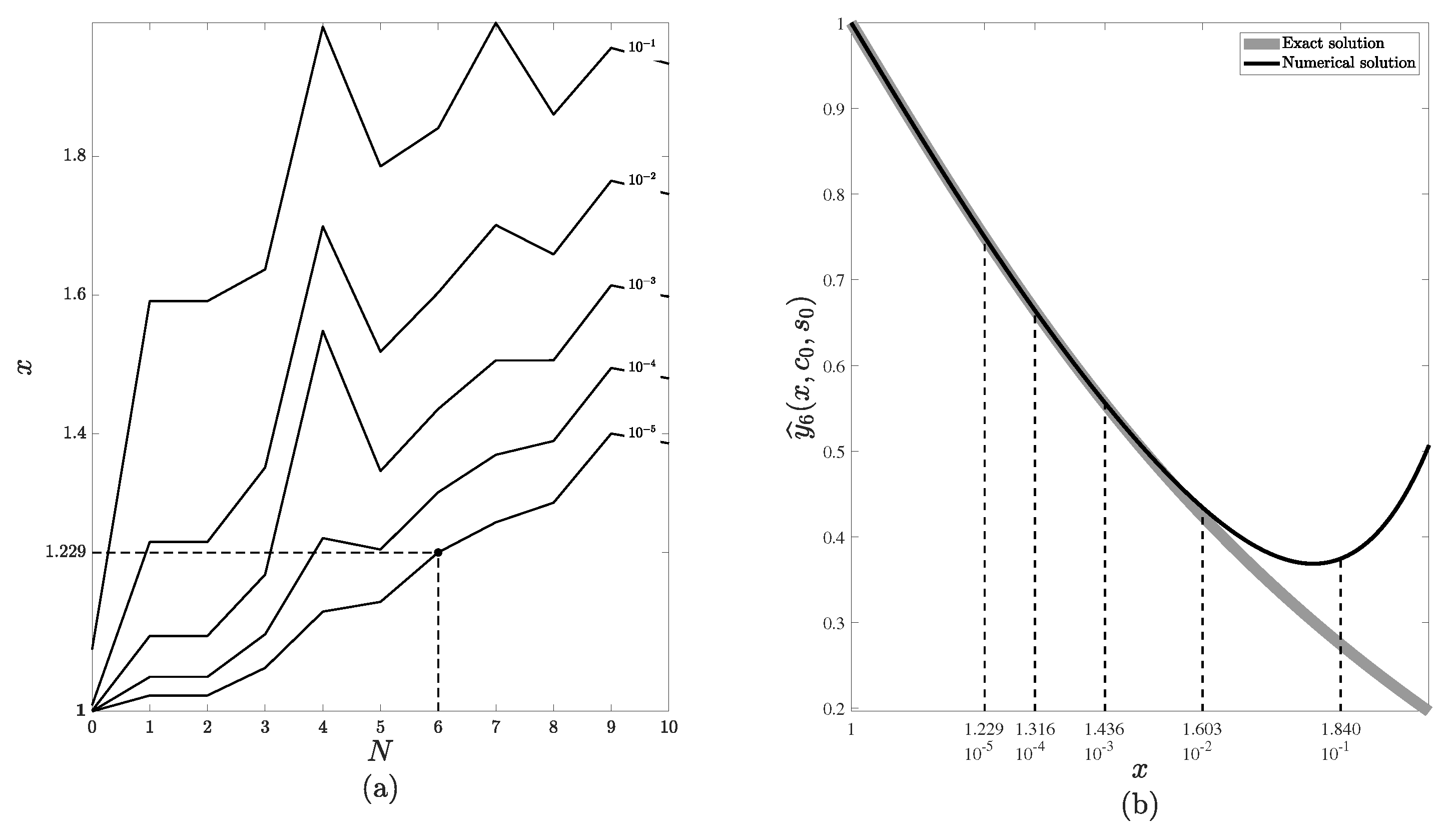
• Step 1. Let $c_0=s_0=1$. The absolute differences ${\Delta }_N(x,c_0,s_0)=|\widehat{y}\left(x\right)-{\widehat{y}}_N(x,c_0,s_0)|$ are computed for $N=0,\cdots ,10$ and $x\in [1,L]$, where L is the upper bound of x. The contour plot depicting various levels of ${\Delta }_N(x,c_0,s_0)$ is presented in Figure 1a. It can be observed that for a fixed value of N the value of ${\Delta }_N(x,c_0,s_0)$ increases as x increases. New initial values $c_1$, $s_1$ for the next approximation are computed as follows:

  $$c_1=\underset{x}{arg\; max}{\Delta }_N(x,c_0,s_0)\le \delta ;s_1={\widehat{y}}_N(c_1,c_0,s_0),$$

  (36)

  where $\delta$ is the maximal allowed error of the numerical solution. Naturally, higher values of N result in larger values of $c_1$ at a cost of greater computation time. Let $N=6$. Then, the resulting values of $c_1$ for different levels of $\delta$ are displayed in Figure 1b (denoted as black dashed lines, while the thick gray line denotes the analytical solution and the black solid line denotes the numerical solution). Figure 1 part (a) contains a contour plot with various levels of ${\Delta }_N(x,c_0,s_0)$ (absolute differences between the exact and numerical solutions to (32)–(33)). Parameter $\delta$ is set to ${10}^{-5}$ for the remainder of this computational experiment, as shown by the point in Figure 1a.
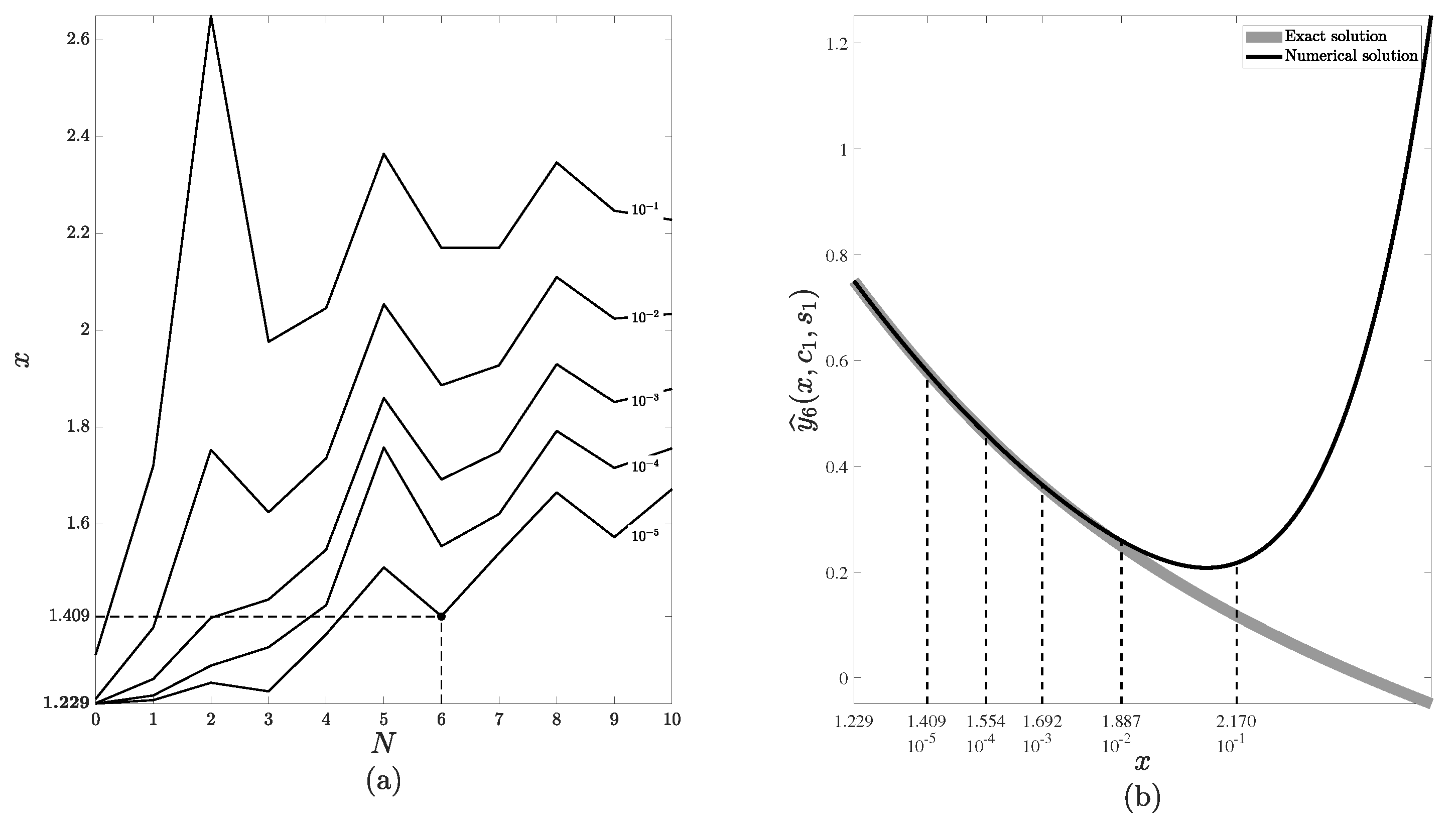
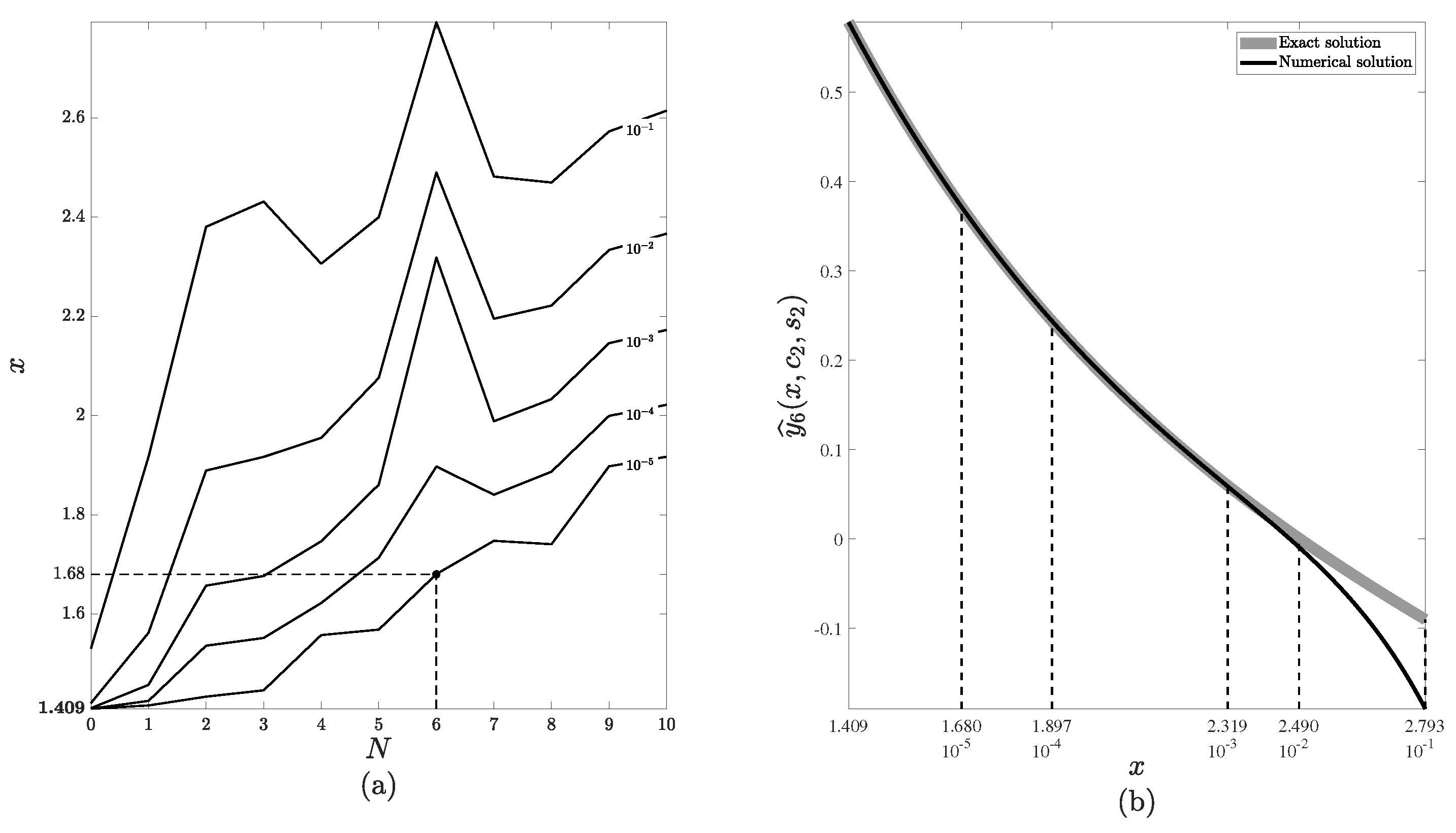
• Step $k=2,3,\cdots ,K$. Analogous computations are performed for steps $k=2,3,\cdots ,K$. Firstly, differences ${\Delta }_N(x,c_{k-1},s_{k-1})=|\widehat{y}\left(x\right)-{\widehat{y}}_N(x,c_{k-1},s_{k-1})|$ are evaluated for $N=0,\cdots ,10$ and $x\in [c_{k-1},L]$ and then new initial values $c_k$, $s_k$ are computed:

  $$c_k=\underset{x}{arg\; max}{\Delta }_N(x,c_{k-1},s_{k-1})\le \delta ;s_1={\widehat{y}}_N(c_k,c_{k-1},s_{k-1}).$$

  (37)
  Results of the steps $k=2,3$ are displayed in Figure 2 and Figure 3.

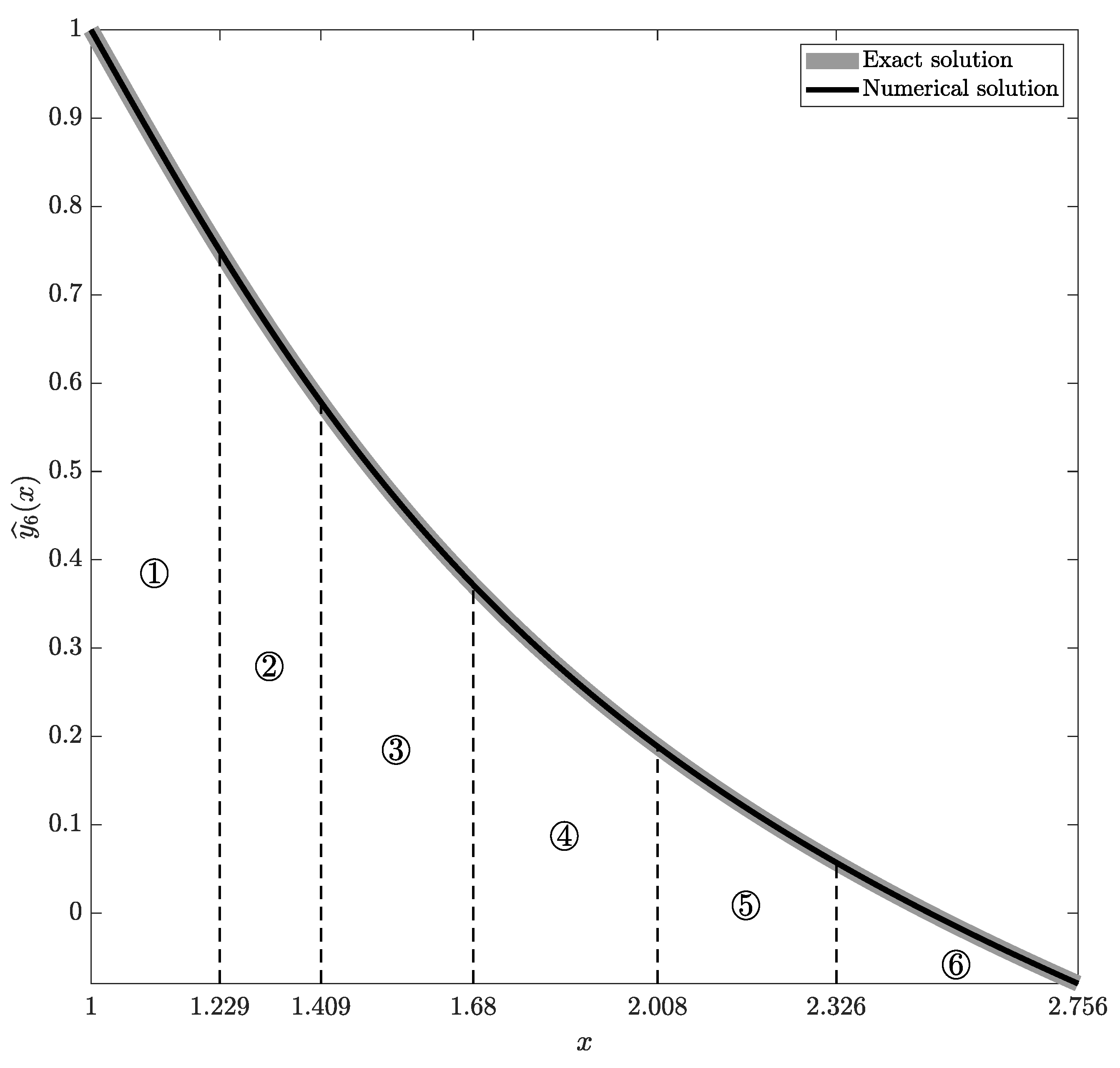
The number of steps K is set to $K=6$ in this study. The final piecewise-polynomial approximation ${\widehat{y}}_N\left(x\right)$ to (32)–(33) is depicted in Figure 4. Let the change in the numerical solution ${\widehat{y}}_N\left(x\right)$ at each step be denoted as

$$\Delta {\widehat{y}}_N^{\left(k\right)}=\underset{c_{k-1}\le x\le c_k}{max}{\widehat{y}}_N(x,c_{k-1},s_{k-1})-\underset{c_{k-1}\le x\le c_k}{min}{\widehat{y}}_N(x,c_{k-1},s_{k-1});k=1,\cdots ,K.$$

(38)

The relationship between $\Delta {\widehat{y}}_N^{\left(k\right)}$ and the step-size $h_k$ can be approximated via the following linear regression line:

$$\Delta {\widehat{y}}_N={\kappa }_0^{\left(N\right)}+{\kappa }_1^{\left(N\right)}h,$$

(39)

where ${\kappa }_0^{\left(N\right)}$, ${\kappa }_1^{\left(N\right)}\in \mathbb{R}$ are regression coefficients. The constructions of linear regressions for $N=6$ and $N=7$ are illustrated in Figure 5 (parts (a) and (b), respectively). Black circles depict the values obtained from the final piecewise-polynomial approximation shown in Figure 4. The digits above the black circles denote the step number. The gray line corresponds to the linear regression (39). Regression equations for $N=6$ (part (a)) and $N=7$ (part (b)) read $\Delta {\widehat{y}}_N=0.26572-0.29293h$ and $\Delta {\widehat{y}}_N=0.27996-0.11987h$, respectively.

All computation steps performed for $N=6$ were also repeated for $N=7$ to obtain the regression depicted in Figure 5b. Note that while the coefficient of h decreases for a higher-order approximation, the overall trend remains unchanged.

The identification of the relationship between the change in the numerical solution and the step-size can be incorporated into the numerical FDE integration scheme that is described in the next section.

3.2. The Implementation of the Numerical FDE Integration Scheme

Let us consider the following fractional differential equation:

$$\begin{array}{cc}\hfill & {\left({}^C{\mathrm{D}}^{1/2}\right)}^{2}y=Q\left(y\right);\hfill \end{array}$$

(40)

$$\begin{array}{cc}\hfill & y\left(x_0\right)=u_0;{\left({}^C{\mathrm{D}}^{1/2}\right)y|}_{x=0}=v_0.\hfill \end{array}$$

(41)

The numerical solution to (40)–(41) can be obtained via the integration scheme presented below:

• Transform the FDE (40)–(41) into the characteristic ODE using the procedure described in Section 2.5:

  $$\begin{array}{cc}\hfill & \frac{\mathrm{d}\widehat{y}}{\mathrm{d}x}=P(\widehat{y},v_0);\hfill \end{array}$$

  (42)

  $$\begin{array}{cc}\hfill & \widehat{y}\left(c_0\right)=s_0.\hfill \end{array}$$

  (43)
• Obtain analytic expressions of coefficients $p_j(c,s)$ in the series solution (35) to the ODE (42)–(43) (see Section 2.1.1).
• Fix the values of the following parameters: the order of the approximation N, the upper bound of the independent variable L, the upper bound for the step-size $h^{\left(U\right)}$, the upper bound for the change in the numerical solution $\Delta {\widehat{y}}_N^{\left(U\right)}$. Note that the recommended values for the parameters $h^{\left(U\right)}$ and $\Delta {\widehat{y}}_N^{\left(U\right)}$ are derived from the study presented in the previous section (Figure 5). The value $h^{\left(U\right)}$ corresponds to the highest value of h on the regression line, while the value $\Delta {\widehat{y}}_N^{\left(U\right)}$ corresponds to the highest value of $\Delta {\widehat{y}}_N$ on the regression line.
• Repeat the following steps until the upper bound L is reached ($k=0,1,2\cdots$):
  • Evaluate coefficients $p_j(c_k,s_k),j=1,\cdots ,N$.
  • Find the lowest value of x at which at least one of the following conditions is violated:

    $$\begin{array}{cc}\hfill & h_k\left(x\right)=x-c_k\le h^{\left(U\right)};\hfill \end{array}$$

    (44)

    $$\begin{array}{cc}\hfill & \Delta {\widehat{y}}_N^{\left(k\right)}\left(x\right)=\underset{c_k\le \tilde{x}\le x}{max}{\widehat{y}}_N(\tilde{x},c_k,s_k)-\underset{c_k\le \tilde{x}\le x}{max}{\widehat{y}}_N(\tilde{x},c_k,s_k)\le \Delta {\widehat{y}}_N^{\left(U\right)};\hfill \end{array}$$

    (45)

    $$\begin{array}{cc}\hfill & \Delta {\widehat{y}}_N^{\left(k\right)}\left(x\right)\le {\kappa }_0^{\left(N\right)}+{\kappa }_1^{\left(N\right)}{h}_k\left(x\right),\hfill \end{array}$$

    (46)

    where ${\kappa }_0^{\left(N\right)}$, ${\kappa }_1^{\left(N\right)}\in \mathbb{R}$ are regression coefficients determined in Section 3.1. The maximum and minimum values in (45) are necessary to ensure that the change in the numerical solution is computed correctly for non-monotonous and periodic functions.
  • Assign new initial values:

    $$c_{k+1}=x-\epsilon ;s_{k+1}={\widehat{y}}_N(c_{k+1},c_k,s_k),$$

    (47)

    where $\epsilon$ is an arbitrary small number.
• Combine the obtained parts of the numerical solution to the ODE (42)–(43) into the piecewise-polynomial approximation ${\widehat{y}}_N\left(x\right)$:

  $${\widehat{y}}_N\left(x\right)={\widehat{y}}_N\left(x,c_k,s_k\right),c_k\le x<c_{k+1},k=0,1,\cdots$$

  (48)
• Construct the numerical solution to the FDE (40)–(41) by applying $y_N\left(x\right)={\widehat{y}}_N\left(\sqrt{x}\right)$.

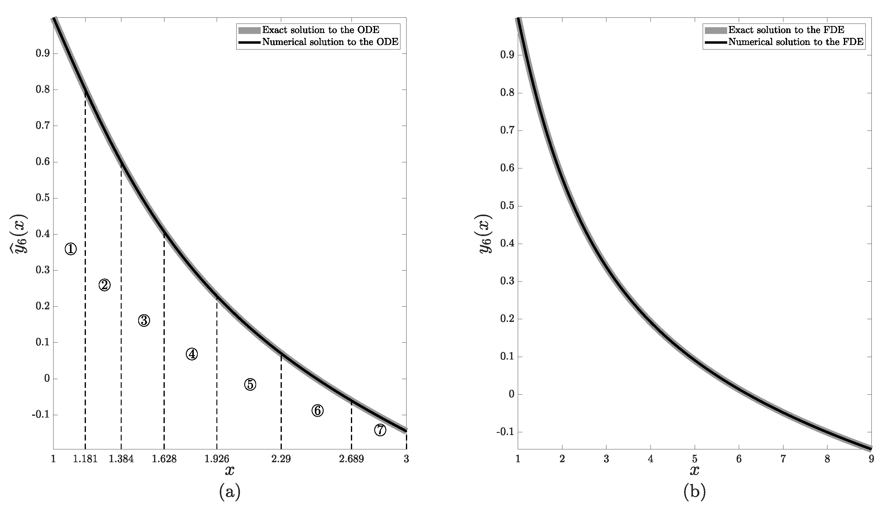
In order to validate the proposed numerical FDE integration scheme, it is applied to the FDE (30)–(31) presented in the previous section. The resulting piecewise-polynomial approximations ${\widehat{y}}_N\left(x\right)$ and $y_N\left(x\right)$ are depicted in Figure 6. Part (a) depicts the exact (gray solid line) and the numerical (black solid line) solutions to the characteristic ODE (32)–(33) ($N=6$, $L=3$, $\delta ={10}^{-5}$). Black dashed lines separate the parts of the numerical solution obtained at different steps. Circled digits denote the step number. Part (b) displays the exact solution (solid gray line) and piecewise-polynomial approximation (black solid line) to the initial FDE (30)–(31).

4. The Application of the Proposed Numerical FDE Integration Scheme

Consider the following fractional Riccati-type equation:

$$\begin{array}{cc}\hfill & x{\left({}^C{\mathrm{D}}^{1/2}\right)}^{2}y=1-2y+y^2-y^3;\hfill \end{array}$$

(49)

$$\begin{array}{cc}\hfill & y\left(1\right)=1;{{}^C{\mathrm{D}}^{1/2}y|}_{x=0}=-1.\hfill \end{array}$$

(50)

Transforming (49)–(50) into the characteristic ODE (see Appendix B for a detailed derivation) yields:

$$\begin{array}{cc}\hfill & \frac{\mathrm{d}\widehat{y}}{\mathrm{d}x}=\frac{2\left(1-2\widehat{y}+{\widehat{y}}^2-{\widehat{y}}^3\right)}{x}-\frac{2}{\sqrt{\pi }};\hfill \end{array}$$

(51)

$$\begin{array}{cc}\hfill & \widehat{y}\left(1\right)=1;\widehat{y}=\widehat{y}\left(x\right);\widehat{y}\left(\sqrt{x}\right)=y\left(x\right).\hfill \end{array}$$

(52)

Note that the FDE (49)–(50) does have a solution (the existence of the solution follows from (26)–(28)). However, the solution to (51)–(52) cannot be expressed in a closed form, because the coefficients $p_j$, as defined in (5), do not form a linear recurring sequence. Furthermore, (51) cannot be transformed via such an independent variable substitution if the coefficients would form a linear recurring sequence. The analytical expressions of coefficients $p_j(c,s),j=0,\cdots ,6$ can be found in Appendix C.

The numerical FDE integration scheme presented in the previous section is used in order to obtain the piecewise-polynomial approximations ${\widehat{y}}_N\left(x\right)$ and $y_N\left(x\right)$ to (51)–(52) and (49)–(50), respectively. The linear regression equation approximating the relationship between the step-size $h_k$ and the change in the numerical solution $\Delta {\widehat{y}}_N^{\left(k\right)}$ derived in Section 3.1 for $N=6$ (Figure 5 part (a)) is used in order to adaptively select the optimal step-size. The resulting numerical solutions ${\widehat{y}}_N\left(x\right)$ and $y_N\left(x\right)$ are displayed in the Figure 7. Part (a) depicts the numerical solution to the characteristic ODE (51)–(52) ($N=6$, $L=3$, $\delta ={10}^{-5}$). Black dashed lines separate the parts of the numerical solution obtained at different steps. Circled digits denote the step number. Part (b) displays the piecewise-polynomial approximation to the initial FDE (49)–(50). The values of $h_k$ and $\Delta {\widehat{y}}_N^{\left(k\right)}$ at each step are presented in

Table 1. The values of the step-size $h_k$ and the variation $\Delta {\widehat{y}}_N^{\left(k\right)}$ in the numerical solution to (51)–(52) at each step $k=1,\cdots ,8$.

Step k	${\mathit{h}}_{\mathit{k}}$	$\Delta {\widehat{\mathit{y}}}_6^{\left(\mathit{k}\right)}$
1	0.080	0.1992
2	0.128	0.1990
3	0.217	0.2000
4	0.311	0.1743
5	0.393	0.1500
6	0.399	0.1185
7	0.399	0.1006
8	0.073	0.0170

.

5. Concluding Remarks

A novel semi-analytical scheme for the numerical integration of fractional differential equations was presented in this paper. The proposed integration scheme is adaptive: the approximation error can be selected arbitrarily, and the algorithm is adapted by using a higher-order piecewise-polynomial approximation. Furthermore, the scheme can easily be extended into higher-order fractional differential equations, since the generalized differential operator technique is applicable to differential systems of any order.

All computational experiments in this paper were performed on fractional Riccati-type nonlinear differential equations. Riccati equations play the central role in nonlinear dynamics because solutions to ordinary Riccati equations do represent soliton-type solutions [28,33]. Without doubt, the proposed scheme can be used for numerical integration of any other class of fractional differential equations.

While the FDEs analyzed in this paper have all had a base derivative order of $\alpha =\frac{1}{2}$ for simplicity, the scheme remains valid for any fractional derivative base order $\alpha =\frac{1}{k}$. This change is implemented by replacing the operator ${}^C{\mathrm{D}}^{1/2}$ with ${}^C{\mathrm{D}}^{1/k}$, while the algorithm to obtain the characteristic ODE remains unchanged except for a higher number of initial conditions.

The presented integration scheme cannot advance past a singularity point. The size of the integration step becomes arbitrarily small as the solution nears the singularity point. This fact can be considered the limitation of the scheme. However, this feature allows the description of the solution in the surrounding of the singularity point with a predefined accuracy.

The extension of the proposed integration scheme to singularity points remains a definite objective for future research. Since the presented scheme is semi-analytical, there are possibilities to adapt it in such a way that singularity points could be detected automatically. Other avenues of future works include adapting the scheme so that any numerical integration technique could be used while solving the characteristic ODE. While this would make the scheme purely numerical and pose challenges in changing the timescale (since the approximation would no longer be a polynomial function), it could potentially open up new possibilities in applying already existing results.

References

- Heymans, N. Fractional calculus description of non-linear viscoelastic behaviour of polymers. Nonlinear Dyn. 2004, 38, 221–231. [Google Scholar] [CrossRef]
- Li, X.; Tian, X. Fractional order thermo-viscoelastic theory of biological tissue with dual phase lag heat conduction model. Appl. Math. Model. 2021, 95, 612–622. [Google Scholar] [CrossRef]
- Dubey, V.P.; Dubey, S.; Kumar, D.; Singh, J. A computational study of fractional model of atmospheric dynamics of carbon dioxide gas. Chaos Solitons Fractals 2021, 142, 110375. [Google Scholar] [CrossRef]
- Acay, B.; Inc, M. Fractional modeling of temperature dynamics of a building with singular kernels. Chaos Solitons Fractals 2021, 142, 110482. [Google Scholar] [CrossRef]
- Chen, Y.; Liu, F.; Yu, Q.; Li, T. Review of fractional epidemic models. Appl. Math. Model. 2021, 97, 281–307. [Google Scholar] [CrossRef]
- Biala, T.A.; Khaliq, A. A fractional-order compartmental model for the spread of the COVID-19 pandemic. Commun. Nonlinear Sci. Numer. Simul. 2021, 98, 105764. [Google Scholar] [CrossRef] [PubMed]
- Rezaei, M.; Yazdanian, A.; Ashrafi, A.; Mahmoudi, S. Numerical pricing based on fractional Black–Scholes equation with time-dependent parameters under the CEV model: Double barrier options. Comput. Math. Appl. 2021, 90, 104–111. [Google Scholar] [CrossRef]
- Tarasov, V.E. Fractional econophysics: Market price dynamics with memory effects. Phys. A Stat. Mech. Appl. 2020, 557, 124865. [Google Scholar] [CrossRef]
- Betancur-Herrera, D.E.; Muñoz-Galeano, N. A numerical method for solving Caputo’s and Riemann-Liouville’s fractional differential equations which includes multi-order fractional derivatives and variable coefficients. Commun. Nonlinear Sci. Numer. Simul. 2020, 84, 105180. [Google Scholar] [CrossRef]
- Alchikh, R.; Khuri, S. Numerical solution of a fractional differential equation arising in optics. Optik 2020, 208, 163911. [Google Scholar] [CrossRef]
- Mendes, E.M.; Salgado, G.H.; Aguirre, L.A. Numerical solution of Caputo fractional differential equations with infinity memory effect at initial condition. Commun. Nonlinear Sci. Numer. Simul. 2019, 69, 237–247. [Google Scholar] [CrossRef]
- Firoozjaee, M.; Jafari, H.; Lia, A.; Baleanu, D. Numerical approach of Fokker–Planck equation with Caputo–Fabrizio fractional derivative using Ritz approximation. J. Comput. Appl. Math. 2018, 339, 367–373. [Google Scholar] [CrossRef]
- Kheybari, S. Numerical algorithm to Caputo type time–space fractional partial differential equations with variable coefficients. Math. Comput. Simul. 2021, 182, 66–85. [Google Scholar] [CrossRef]
- Esmaeili, S.; Shamsi, M.; Luchko, Y. Numerical solution of fractional differential equations with a collocation method based on Müntz polynomials. Comput. Math. Appl. 2011, 62, 918–929. [Google Scholar] [CrossRef] [Green Version]
- Han, W.; Chen, Y.M.; Liu, D.Y.; Li, X.L.; Boutat, D. Numerical solution for a class of multi-order fractional differential equations with error correction and convergence analysis. Adv. Differ. Equ. 2018, 2018, 1–22. [Google Scholar] [CrossRef]
- Hinze, M.; Schmidt, A.; Leine, R.I. Numerical solution of fractional-order ordinary differential equations using the reformulated infinite state representation. Fract. Calc. Appl. Anal. 2019, 22, 1321–1350. [Google Scholar] [CrossRef]
- Maleknejad, K.; Rashidinia, J.; Eftekhari, T. Numerical solutions of distributed order fractional differential equations in the time domain using the Müntz–Legendre wavelets approach. Numer. Methods Partial Differ. Equ. 2021, 37, 707–731. [Google Scholar] [CrossRef]
- Babaaghaie, A.; Maleknejad, K. Numerical solutions of nonlinear two-dimensional partial Volterra integro-differential equations by Haar wavelet. J. Comput. Appl. Math. 2017, 317, 643–651. [Google Scholar] [CrossRef]
- Garrappa, R. Numerical solution of fractional differential equations: A survey and a software tutorial. Mathematics 2018, 6, 16. [Google Scholar] [CrossRef] [Green Version]
- Jafari, H.; Tajadodi, H. He’s variational iteration method for solving fractional Riccati differential equation. Int. J. Differ. Equ. 2010, 2010, 764738. [Google Scholar] [CrossRef] [Green Version]
- Khan, N.A.; Ara, A.; Jamil, M. An efficient approach for solving the Riccati equation with fractional orders. Comput. Math. Appl. 2011, 61, 2683–2689. [Google Scholar] [CrossRef] [Green Version]
- Gohar, M. Approximate Solution to Fractional Riccati Differential Equations. Fractals 2019, 27, 1950128. [Google Scholar] [CrossRef]
- Timofejeva, I.; Navickas, Z.; Telksnys, T.; Marcinkevičius, R.; Yang, X.J.; Ragulskis, M.K. The extension of analytic solutions to FDEs to the negative half-line. AIMS Math. 2021, 6, 3257–3271. [Google Scholar] [CrossRef]
- Navickas, Z.; Bikulciene, L.; Ragulskis, M. Generalization of Exp-function and other standard function methods. Appl. Math. Comput. 2010, 216, 2380–2393. [Google Scholar] [CrossRef]
- Navickas, Z.; Marcinkevicius, R.; Telksnys, T.; Ragulskis, M. Existence of second order solitary solutions to Riccati differential equations coupled with a multiplicative term. IMA J. Appl. Math. 2016, 81, 1163–1190. [Google Scholar] [CrossRef]
- Kurakin, V.; Kuzmin, A.; Mikhalev, A.; Nechaev, A. Linear recurring sequences over rings and modules. J. Math. Sci. 1995, 76, 2793–2915. [Google Scholar] [CrossRef]
- Zaitsev, V.F.; Polyanin, A.D. Handbook of Exact Solutions for Ordinary Differential Equations; CRC Press: Boca Raton, FL, USA, 2002. [Google Scholar]
- Navickas, Z.; Ragulskis, M. How far one can go with the Exp-function method? Appl. Math. Comput. 2009, 211, 522–530. [Google Scholar] [CrossRef]
- Andrews, G.E.; Askey, R.; Roy, R. Special Functions; Number 71; Cambridge University Press: Cambridge, MA, USA, 1999. [Google Scholar]
- Navickas, Z.; Telksnys, T.; Timofejeva, I.; Marcinkevičius, R.; Ragulskis, M. An operator-based approach for the construction of closed-form solutions to fractional differential equations. Math. Model. Anal. 2018, 23, 665–685. [Google Scholar] [CrossRef]
- Zhou, Y.; Wang, J.; Zhang, L. Basic Theory of Fractional Differential Equations; World Scientific: Singapore, 2016. [Google Scholar]
- Navickas, Z.; Telksnys, T.; Marcinkevicius, R.; Ragulskis, M. Operator-based approach for the construction of analytical soliton solutions to nonlinear fractional-order differential equations. Chaos Solitons Fractals 2017, 104, 625–634. [Google Scholar] [CrossRef]
- Scott, A. Encyclopedia of Nonlinear Science; Routledge: Abingdon-on-Thames, UK, 2006. [Google Scholar]
Figure 1.
The determination of the second set of initial values for the numerical solution (35). The first set of initial values is , . Part (a) depicts a contour plot of the error for different values of N. Part (b) depicts the next initial points for different errors for .
Figure 2.
The determination of the third set of initial values for the numerical solution (35). The second set of initial values is , . Part (a) depicts a contour plot of the error for different values of N. Part (b) depicts the next initial points for different errors for .
Figure 3.
The determination of the fourth set of initial values for the numerical solution (35). The third set of initial values is , . Part (a) depicts a contour plot of the error for different values of N. Part (b) depicts the next initial points for different errors for .
Figure 4.
Gray and black solid lines correspond to the exact solution and the piecewise-polynomial approximation to (32)–(33), respectively (, ). Black dashed lines separate the parts of the numerical solution obtained at different steps. Circled digits denote the step number.
Figure 5.
The relationship between (the change in the numerical solution ) and the step-size h. Parts (a,b) correspond to and , respectively.
Figure 6.
The application of the numerical FDE integration scheme to (30)–(31). Part (a) depicts the exact and approximate solutions to the characteristic ODE, while part (b) depicts the exact and approximate solutions to the FDE.
Figure 7.
The application of the numerical FDE integration scheme to (49)–(50). Part (a) depicts the exact and approximate solutions to the characteristic ODE, while part (b) depicts the exact and approximate solutions to the FDE.
Publisher’s Note: MDPI stays neutral with regard to jurisdictional claims in published maps and institutional affiliations. |
© 2021 by the authors. Licensee MDPI, Basel, Switzerland. This article is an open access article distributed under the terms and conditions of the Creative Commons Attribution (CC BY) license (https://creativecommons.org/licenses/by/4.0/).
Share and Cite
MDPI and ACS Style
Timofejeva, I.; Navickas, Z.; Telksnys, T.; Marcinkevicius, R.; Ragulskis, M. An Operator-Based Scheme for the Numerical Integration of FDEs. Mathematics 2021, 9, 1372. https://doi.org/10.3390/math9121372
AMA Style
Timofejeva I, Navickas Z, Telksnys T, Marcinkevicius R, Ragulskis M. An Operator-Based Scheme for the Numerical Integration of FDEs. Mathematics. 2021; 9(12):1372. https://doi.org/10.3390/math9121372
Chicago/Turabian StyleTimofejeva, Inga, Zenonas Navickas, Tadas Telksnys, Romas Marcinkevicius, and Minvydas Ragulskis. 2021. "An Operator-Based Scheme for the Numerical Integration of FDEs" Mathematics 9, no. 12: 1372. https://doi.org/10.3390/math9121372
Note that from the first issue of 2016, this journal uses article numbers instead of page numbers. See further details here.