An Alternative Promotion Time Cure Model with Overdispersed Number of Competing Causes: An Application to Melanoma Data

Abstract

A cure rate model under the competing risks setup is proposed. For the number of competing causes related to the occurrence of the event of interest, we posit the one-parameter Bell distribution, which accommodates overdispersed counts. The model is parameterized in the cure rate, which is linked to covariates. Parameter estimation is based on the maximum likelihood method. Estimates are computed via the EM algorithm. In order to compare different models, a selection criterion for non-nested models is implemented. Results from simulation studies indicate that the estimation method and the model selection criterion have a good performance. A dataset on melanoma is analyzed using the proposed model as well as some models from the literature.

1. Introduction

The usual approach in models for time-to-event data is built on the assumption that all subjects will experience the event of interest if the follow-up time is long enough. In many studies in different areas, there are subjects insusceptible to the event of interest. We call cure rate the proportion of insusceptible subjects. Cure rate models, also known as long-term survival models, are capable to deal with this situation.

Cure rate models have had an intense research activity in last years. From the seminal contributions in [1,2] and the approach based on competing risks for cure rate models in [3], we find many papers in recent years on this research area. The competing risks approach is summarized as follows. Let M be an unobserved variable denoting the initial number of competing causes related to the occurrence of the event of interest. For instance, in cancer studies M represents the number of carcinogenic cells at the end of treatment that can produce a detectable cancer. For M following the Bernoulli or the Poisson distribution, we obtain the models in [2,3], respectively. The time for the j-th competing cause to produce the event of interest (that is, the promotion time) is denoted by $Z_j$, $j=1,\dots ,M$. We also assume that, conditional on M, the latent times $Z_1,\dots ,Z_M$ are independent and identically distributed with cumulative distribution function (cdf) $F(z;\mathbf{\lambda })$ and survival function $S(z;\mathbf{\lambda })=1-F(z;\mathbf{\lambda })$, where $\mathbf{\lambda }$ is the parameter vector. Under a competing risks setup, the time elapsed until the event of interest is given by $T=min(Z_0,Z_1,\dots ,Z_M)$, where $Z_0$ is a random variable degenerate at $+\infty$. Our paper is based on the competing risks approach for cure rate models.

Many cure rate models proposed in last years are formulated from different distributions for the number of competing causes M. This research line includes the negative binomial [4], COM-Poisson [5], power series [6], Yule-Simon [7], polylogarithm [8], modified power series [9], zero inflated power series [10] and zero-modified geometric [11] distributions, among many others. In this vein, we adopt the one-parameter Bell distribution recently proposed in [12], with probability mass function (pmf)

$$P(M=m;\theta )=\frac{B_m{\theta }^m{e}^{-e^{\theta }+1}}{m!},m=0,1,2,\dots ,$$

(1)

for $\theta >0$, where $B_m$ is the Bell number defined as $B_m=e^{-1}{\sum }_{k=0}^{\infty }{k}^m/k!$. The first few Bell numbers are $B_0=B_1=1,B_2=2,B_3=5,B_4=15,B_5=52,B_6=203,$ $B_7=877,B_8=4140,B_9=21147$ and $B_{10}=115975$. We denote $M\sim \mathrm{Bell}\left(\theta \right)$ to say that M follows a distribution with pmf in (1). Denoting the mean and the variance of M by $\mathbb{E}\left(M\right)$ and Var$\left(M\right)$, respectively, we have that $\mathbb{E}\left(M\right)=\theta e^{\theta }$ and Var$\left(M\right)=\theta (1+\theta )e^{\theta }$. Since Var$\left(M\right)>\mathbb{E}\left(W\right)$, the Bell distribution accommodates overdispersed counts. For cure rate models, this distribution is interesting due to some characteristics:

• The distribution has only one parameter, being an alternative to traditional discrete distributions such as Poisson and Geometric.
• The probability generating function (pgf) of the distribution has a simple expression. In fact, if $M\sim \mathrm{Bell}\left(\theta \right)$, then its pgf is given by $G(s;\theta )=exp(e^{\theta s}-e^{\theta })$, for $\left|s\right|<1$. See Proposition 1 in [12]. This fact is relevant from the point of view of cure rate models because the population survival function depends on this function.
• $P(M=0;\theta )=exp(-e^{\theta }+1)$ has a simple form. This fact is important because this probability is the cure rate of the model. The simplicity of this term allows, among other things, to reparameterize the model in terms of the cure rate.
• The distribution belongs to the power series family of distributions [13] with pmf $P(M=m;\theta )=a_m{\theta }^m/A\left(\theta \right)$, where $a_m=B_m/m!$, $m=0,1,2,\dots$, and $A\left(\theta \right)={\sum }_{m=0}^{\infty }{a}_m{\theta }^m=exp(e^{\theta }-1)$. Recently, ref. [14] proposed an EM-type algorithm for a class of cure rate models based on the power series family. The maximization (M) step of the EM algorithm is decomposed in two steps involving the distribution of the number of competing causes M and the distribution of the latent times Z.
• To the best of our knowledge, the Bell distribution has not yet been proposed to model the number of competing causes in a cure rate models context.

The remaining of the paper is organized as follows. In Section 2, we present the cure rate rate model. Inference methods are presented in Section 3. Section 4 is dedicated to a simulation study covering properties of the estimators and model selection. A dataset on melanoma is analyzed in Section 5. Closing remarks are given in Section 6.

2. Model

Let M be an unobserved variable denoting the initial number of competing causes related to the occurrence of an event of interest. We assume that $M\sim \mathrm{Bell}\left(\theta \right)$. Under the competing risks setup in Section 1, from Theorem 2 in [4], see also [15], we have that the (improper) population survival function of the Bell cure rate (Bellcr) model is given by

$$S_{pop}(t;\theta ,\mathbf{\lambda })=P(T>t;\theta ,\mathbf{\lambda })=G\left(S(t;\mathbf{\lambda });\theta \right)=exp[e^{\theta S(t;\mathbf{\lambda })}-e^{\theta }].$$

(2)

It is immediate that the cure rate of the model is given by $p={lim}_{t\to \infty }{S}_{pop}(t;\mathbf{\psi })=exp(1-e^{\theta })=P(M=0;\theta )$. Henceforth, we adopt the parameterization $p=exp(1-e^{\theta })$, i.e., $\theta =log[1-log(p\left)\right]$. In this way, covariates can be directly linked to the cure rate p, allowing to compare regression coefficients among different models parameterized in terms of the cure rate.

An interesting family of cure rate models parameterized in the cure rate is studied in [16]. Such family includes the Bernoulli cure rate (Berncr) model, also known as mixture cure model [1,2], the Poisson cure rate (Pocr) model, also known as the promotion time cure model [3,17], the logarithmic cure rate (Locr) model and the negative binomial cure rate (NBcr) model, noticing that the NBcr model has an additional parameter q$(q>0)$ and $q=1$ corresponds to the geometric cure rate (Geocr) model.

Table 1. Variance of the number of competing causes as a function of the cure rate for some models parameterized in the cure rate (p).

Model	Var$\left(\mathit{M}\right)$	Model	Var$\left(\mathit{M}\right)$
Berncr	$p(1-p)$	NBcr	$q(1-p^{1/q})p^{-2/q}$
Pocr	$-log\left(p\right)$	Locr *	$\theta [\theta +log(1-\theta )]/{[(1-\theta )log(1-\theta )]}^2$
Geocr	$(1-p)p^{-2}$	Bellcr	$[1-log(p\left)\right]log[1-log(p\left)\right]\{1+log[1-log\left(p\right)\left]\right\}$

* $\theta =\theta \left(p\right)=1+pW[-exp(-1/p)/p]$, where $W(·)$ denotes the Lambert function  [18].

and Figure 1 show the variance of the number of competing causes M in terms of the cure rate for some models. Note that the curve for the Bellcr model lies between the Geocr and Pocr models. Also, the curves for the NBcr model with q = 0.3, 5 and 10 are close to the Locr, Bellcr and Pocr models, respectively. In fact, by applying the L’Hopital’s rule, we have ${lim}_{q\to \infty }q(1-p^{1/q})p^{-2/q}=-log\left(p\right)$ so that the proximity between the NBcr$(q=10)$ and Pocr curves is justified.

With the parameterization in the cure rate p, the population survival function for the Bellcr model in (2) is recast, leading to

$$S_{pop}(t;p,\mathbf{\lambda })=pexp\{{\left[1-log\left(p\right)\right]}^{S(t;\mathbf{\lambda })}-1\},$$

(3)

so that the population density and hazard functions are given by

$$f_{pop}(t;p,\mathbf{\lambda })=S_{pop}(t;p,\mathbf{\lambda }){[1-log\left(p\right)]}^{S(t;\mathbf{\lambda })}log[1-log\left(p\right)]f(t;\mathbf{\lambda })$$

(4)

$$\mathrm{and}{h}_{pop}(t;p,\mathbf{\lambda })={[1-log\left(p\right)]}^{S(t;\mathbf{\lambda })}log[1-log\left(p\right)]f(t;\mathbf{\lambda }).$$

In a sample of size n, for the i-th subject the covariates are represented by $x_i={(1,x_{1i},\dots ,x_{ri})}^{\top }$, $i=1,\dots ,n$, where the symbol “⊤” denotes the transpose operator. The cure rate $p_i$ is linked to $x_i$ through the logistic function, that is,

$$log\left(\frac{p_i}{1-p_i}\right)=x_i^{\top }\mathbf{\beta },$$

(5)

where $\mathbf{\beta }={({\beta }_0,{\beta }_1,\dots ,{\beta }_r)}^{\top }$ is the vector of regression coefficients of dimension $r+1$. Therefore, interpretations about the regression coefficients can be obtained in terms of the odds ratio for the cure probability.

3. Inference

In this section, we present some details about the estimation procedure for the parameters of the model in Section 2. We consider a framework in which the lifetimes are subject to right censoring. Let $Y_i$ and $C_i$ be the failure and censoring time variables for the i-th subject, respectively. In a sample of size n, the observed variables are $T_i=min(Y_i,C_i)$ and ${\delta }_i=I(Y_i\le C_i)$, where ${\delta }_i=1$ and ${\delta }_i=0$ denote either if a failure or a censored time was observed for the i-th subject, respectively, $i=1,\dots ,n$. Under the usual assumption of non-informative censoring and with $p_i$ as in (5), the log-likelihood function of $\mathbf{\psi }={({\mathbf{\beta }}^{\top },{\mathbf{\lambda }}^{\top })}^{\top }$ is given by

$$\begin{array}{cc}\hfill \ell \left(\mathbf{\psi }\right)& =\sum _{i=1}^n(log\left(p_i\right)+log\{{[1-log\left(p_i\right)t]}^{S(t;\mathbf{\lambda })}-1\}+{\delta }_i\{S(t_i;\mathbf{\lambda })log[1-log\left(p_i\right)]\hfill \\ \hfill & +log\{(log[1-log\left(p_i\right)]\}+log\left[f(t_i;\mathbf{\lambda })\right]\}).\hfill \end{array}$$

(6)

The maximum likelihood (ML) estimator of $\mathbf{\psi }$, $\widehat{\mathbf{\psi }}$ say, is obtained by maximizing (6) with respect to $\mathbf{\psi }$. However, direct maximization is not computationally simple because some terms in (6) involve both $\mathbf{\beta }$ and $\mathbf{\lambda }$. For this reason and taking advantage of the EM algorithm developed for the power series family of cure rate models in [14], ML estimates in the Bellcr model are computed using this algorithm. In short, the k-th iteration of the EM algorithm goes as follows:

• E step: For $i=1,\dots ,n$, compute ${\tilde{M}}_i^{\left(k\right)}={\mu }_i^{(k-1)}exp\left({\mu }_i^{(k-1)}\right)+{\delta }_i(1+{\mu }_i^{(k-1)})$, where ${\mu }_i^{(k-1)}={\theta }_i^{(k-1)}S(t_i;{\mathbf{\lambda }}^{(k-1)})$ with ${\theta }_i^{(k-1)}=log[1-log\left(p_i^{(k-1)}\right)]$ and $p_i^{(k-1)}$ comes from (5).
• M step 1: Given ${\tilde{M}}^{\left(k\right)}={({\tilde{M}}_1^{\left(k\right)},\dots ,{\tilde{M}}_n^{\left(k\right)})}^{\top }$, find ${\mathbf{\beta }}^{\left(k\right)}$ that maximizes $Q_1\left(\mathbf{\beta }\right|{\mathbf{\psi }}^{\left(k\right)})$ with respect to $\mathbf{\beta }$, where

  $$Q_1\left(\mathbf{\beta }\right|{\mathbf{\psi }}^{\left(k\right)})=\sum _{i=1}^n\left({\tilde{M}}_i^{\left(k\right)}log\{log[1-log\left(p_i\right)]\}-log\left(p_i\right)\right).$$

  (7)
• M step 2: Given ${\tilde{M}}^{\left(k\right)}$, find ${\mathbf{\lambda }}^{\left(k\right)}$ that maximizes $Q_2\left(\mathbf{\lambda }\right|{\mathbf{\psi }}^{\left(k\right)})$ with respect to $\mathbf{\lambda }$, where

  $$Q_2\left(\mathbf{\lambda }\right|{\mathbf{\psi }}^{\left(k\right)})=\sum _{i=1}^n\{{\tilde{M}}_i^{\left(k\right)}log\left[S(t_i;\mathbf{\lambda })\right]+{\delta }_{i}log\left[h(t_i;\mathbf{\lambda })\right]\}.$$

  (8)

The E and M steps are cycled until a suitable convergence criterion is attained, for instance, $\left|\right|{\mathbf{\psi }}^{\left(k\right)}-{\mathbf{\psi }}^{(k-1)}\left|\right|<ϵ$, where “$\left|\right|·\left|\right|$” denotes the Euclidean norm and $ϵ$ is a specified tolerance. Maximization of the functions in (7) and (8) can be performed using the optim function in R language [19].

We stress that the proposed EM algorithm procedure is general in the sense that it can accommodate different distributions for the latent time Z in Section 1. In this work, we assume the Weibull distribution, denoted by Wei$(\alpha ,\nu )$, because it is a suitable model in a cure rate model context. With $\mathbf{\lambda }={(\alpha ,\nu )}^{\top }$, the survival function for this distribution is given by $S(t;\mathbf{\lambda })=exp\left(-e^{\alpha }{t}^{\nu }\right)$, for $t>0$, $\nu >0$ and $\alpha \in \mathbb{R}$.

On the other hand, the normal theory asymptotic covariance matrix of the maximum likelihood estimator $\widehat{\mathbf{\psi }}$ can be estimated from minus the Hessian matrix of the log-likelihood function in (6) evaluated at $\mathbf{\psi }=\widehat{\mathbf{\psi }}$. The numDeriv R package [20] provides a numerical approximation to this matrix. Interval estimates of the parameters are computed from the asymptotic standard errors. Computational codes are available from the authors upon request.

Finally, inference usually is made on the cure rate. However, we might also be interested in the cure rate for subjects who survived up to a certain time $t_0$, denoted by $p_{t_0}$. First, for $t>t_0$, from (3) we have $P(T>t\mid T>t_0)=P(T>t)/P(T>t_0)=S_{pop}(t;p,\mathbf{\lambda })/S_{pop}(t_0;p,\mathbf{\lambda })=exp\{{[1-log\left(p\right)]}^{S(t;\mathbf{\lambda })}-{[1-log\left(p\right)]}^{S(t_0;\mathbf{\lambda })}\}$. Then, omitting the dependence on the covariates and passing to the limit for $t\to \infty$ we obtain the conditional cure rate

$$p_{t_0}=\underset{t\to \infty }{lim}P(T>t)/P(T>t_0)=exp\{1-{[1-log\left(p\right)]}^{S(t_0;\mathbf{\lambda })}\}.$$

(9)

Of course, if $t_0=0$ in (9), $p_{t_0}$ reduces to the cure rate p in (5). For comparatives purposes, Remark 1 gives expressions for $p_{t_0}$ under the Pocr, Locr, NBcr and Bincr models.

Remark 1.

For the Pocr, Locr, NBcr and Bincr models, routine calculation shows that $p_{t_0}$ is given by

$$\begin{array}{cc}\hfill p_{t_0}& =p^{S(t_0;\mathbf{\lambda })},for the Pocr model,\hfill \\ \hfill p_{t_0}& ={\left(1-(1-p^{1/q})S(t_0;\mathbf{\lambda })\right)}^q,for the NBcr model,\hfill \\ \hfill p_{t_0}& ={\left(1+(1/p-1)S(t_0;\mathbf{\lambda })\right)}^{-q},for the Bincr model and\hfill \\ \hfill p_{t_0}& =\frac{-\theta \left(p\right)S(t_0;\mathbf{\lambda })}{log\left(1-\theta \left(p\right)S(t_0;\mathbf{\lambda })\right)},for the Locr model,\hfill \end{array}$$

where $\theta \left(p\right)=1+pW[-exp(-1/p)/p]$.

4. Simulation Studies

In this section, we present two simulation studies. The main goal of the first study is to assess the performance of the ML estimates for the parameters of the Bellcr model computed with the EM algorithm in Section 3. The second study is devoted to model selection based on Vuong’s test statistic in [21] (see Appendix A) when the true cure rate model is the Bellcr model or may be wrongly specified. The null hypothesis states that the two compared models are undistinguishable. If the null hypothesis is rejected, the model with the highest value of the likelihood function is preferable. We pick a model with three covariates $x_1$, $x_2$ and $x_3$. Figure 2 shows the scheme to draw the covariates.

The true value of $\mathbf{\beta }={({\beta }_0,{\beta }_1,{\beta }_2,{\beta }_3)}^{\top }$ is computed from four combinations of values of $(x_1,x_2,x_3)$ and cure rates $p_{c1},\dots ,p_{c4}$. For $(x_1,x_2,x_3)$, we choose $(0,0,0)$, $(1,0,0)$, $(0,5,2)$ and $(1,10,5)$. Solving the equations in (5), we get ${\beta }_0=\mathrm{logit}\left(p_{c1}\right)$, ${\beta }_1=-\mathrm{logit}\left(p_{c1}\right)+\mathrm{logit}\left(p_{c2}\right)$, ${\beta }_2=-\mathrm{logit}\left(p_{c1}\right)+(2/5)\mathrm{logit}\left(p_{c2}\right)+\mathrm{logit}\left(p_{c3}\right)-(2/5)\mathrm{logit}\left(p_{c4}\right)$ and ${\beta }_3=2$ $\mathrm{logit}\left(p_{c1}\right)-\mathrm{logit}\left(p_{c2}\right)-2\mathrm{logit}\left(p_{c3}\right)+\mathrm{logit}\left(p_{c4}\right)$, where $\mathrm{logit}\left(p\right)=log\left(p\right)-log(1-p)$, for $p\in (0,1)$. In the studies presented here, cure rates $(p_{c1},\dots ,p_{c4})$ are $(0.9,0.8,0.65,0.5)$, $(0.8,0.7,0.55,0.4)$ and $(0.7,0.6,0.45,0.3)$, labeled as Cure 1, Cure 2 and Cure 3, respectively. On the other hand, to set the vector $\mathbf{\lambda }={(\alpha ,\nu )}^{\top }$ we choose values for the expected value $\mathbb{E}\left(Z\right)$ and the variance Var$\left(Z\right)$ of the latent time Z in Section 1. For the Wei$(\alpha ,\nu )$ distribution in Section 3, these conditions imply that $\alpha =\nu \{log[\mathrm{\Gamma }(1+1/\nu )]-log[\mathbb{E}\left(Z\right)\left]\right\}$ and $\nu$ is the solution to the equation $\mathrm{\Gamma }(1+2/\nu )/{\mathrm{\Gamma }}^2(1+1/\nu )=1+\mathrm{Var}\left(Z\right)/{\left[\mathbb{E}\left(Z\right)\right]}^2$.

Table 2. True values of the parameters in the simulation studies.

Cure Rate	${\mathit{\beta }}_0$	${\mathit{\beta }}_1$	${\mathit{\beta }}_2$	${\mathit{\beta }}_3$		$\left(\mathbb{E}\right(\mathit{Z})$, Var$\left(\mathit{Z}\right))$	$\mathit{\alpha }$	$\mathit{\nu }$
Cure 1	2.197	−0.811	−1.024	1.770		(7 , 4)	−8.018	3.920
Cure 2	1.386	−0.539	−0.684	1.118		(5 , 3)	−5.444	3.165
Cure 3	0.847	−0.442	−0.547	0.843		(2 , 1)	−1.712	2.101

showcases the true values of the parameters for the simulations.

The simulations comprise two sample sizes, $n=200$ and $n=400$, and two cases for the latent time Z in Section 1, namely, (i) $\mathbb{E}\left(Z\right)=7$ and Var$\left(Z\right)=4$ and (ii) $\mathbb{E}\left(Z\right)=5$ and Var$\left(Z\right)=3$. For each combination of sample size, cure rate $(p_{c1},\dots ,p_{c4})$ and $\left(\mathbb{E}\left(Z\right),\mathrm{Var}\left(Z\right)\right)$, we compute ${\theta }_i=log[1-log\left(p_i\right)]$, with $p_i$ as in (5). Next, $M_i$ is drawn from the Bell$\left({\theta }_i\right)$ distribution. If $M_i=0$, the failure time is $T_i=+\infty$. If $M_i\ge 1$, we draw $Z_1,\dots ,Z_{M_i}$ from the Wei$(\alpha ,\nu )$ distribution and the failure time is $T_i=min(Z_1,\dots ,Z_{M_i})$. The censoring time $C_i$ is sampled from the $U(0,15)$ distribution. A simulated dataset is formed by $x_i={(1,x_{1i},x_{2i},x_{3i})}^{\top }$, $Y_i=min(T_i,C_i)$ and ${\delta }_i=I(T_i\le C_i)$, $i=1,\dots ,n$. For the Pocr, Locr, NBcr, Geocr and Berncr models in Section 4.2, the data generation process is similar.

Each scenario was replicated 1000 times. The average proportion of censored times ranges from 56% to 77%. The vectors of covariates $x_i$, $i=1,\dots ,n$, are kept fixed throughout the replications.

4.1. Estimation

Having in mind the goal of assessing the behavior of the ML estimates of the parameters in the Bellcr model,

Table 3. Simulated bias (Bias), average of the asymptotic standard errors (SE), root of the simulated mean squared error (RMSE) and coverage probability of the 95% asymptotic confidence intervals (CP) for the Bellcr model.

Cure Rate	$\left(\mathbb{E}\right(\mathbf{Z})$, Var$\left(\mathbf{Z}\right)$)	Parameter	$\mathit{n}=200$				$\mathit{n}=400$
			Bias	SE	RMSE	CP	Bias	SE	RMSE	CP
Cure 1	(7, 4)	${\beta }_0$	0.109	0.594	0.659	0.945	0.046	0.403	0.422	0.952
		${\beta }_1$	−0.003	0.692	0.737	0.949	−0.003	0.471	0.474	0.954
		${\beta }_2$	−0.067	0.210	0.257	0.963	−0.027	0.138	0.143	0.950
		${\beta }_3$	0.112	0.396	0.467	0.957	0.049	0.260	0.269	0.955
		$\alpha$	−0.335	0.823	0.898	0.953	−0.221	0.572	0.647	0.951
		$\nu$	0.164	0.446	0.487	0.951	0.107	0.307	0.339	0.951
	(5, 3)	${\beta }_0$	0.118	0.532	0.597	0.944	0.050	0.363	0.383	0.948
		${\beta }_1$	0.006	0.621	0.641	0.958	0.005	0.427	0.451	0.949
		${\beta }_2$	−0.057	0.183	0.208	0.950	−0.021	0.123	0.132	0.950
		${\beta }_3$	0.082	0.344	0.366	0.955	0.023	0.232	0.247	0.949
		$\alpha$	−0.206	0.518	0.563	0.943	−0.124	0.361	0.397	0.946
		$\nu$	0.111	0.321	0.348	0.943	0.073	0.223	0.237	0.945
Cure 2	(7, 4)	${\beta }_0$	0.043	0.471	0.501	0.945	0.021	0.323	0.323	0.953
		${\beta }_1$	0.005	0.590	0.600	0.955	−0.003	0.408	0.434	0.953
		${\beta }_2$	−0.035	0.139	0.147	0.950	−0.015	0.095	0.100	0.950
		${\beta }_3$	0.058	0.268	0.288	0.941	0.028	0.183	0.191	0.945
		$\alpha$	−0.276	0.820	0.889	0.940	−0.132	0.569	0.590	0.949
		$\nu$	0.137	0.431	0.458	0.947	0.069	0.298	0.309	0.952
	(5, 3)	${\beta }_0$	0.051	0.421	0.433	0.948	0.020	0.291	0.288	0.952
		${\beta }_1$	−0.019	0.534	0.552	0.956	−0.001	0.369	0.390	0.951
		${\beta }_2$	−0.026	0.124	0.127	0.964	−0.013	0.086	0.087	0.950
		${\beta }_3$	0.045	0.240	0.248	0.951	0.022	0.165	0.171	0.950
		$\alpha$	−0.146	0.514	0.534	0.944	−0.078	0.358	0.360	0.953
		$\nu$	0.090	0.311	0.324	0.948	0.051	0.216	0.220	0.952
Cure 3	(7, 4)	${\beta }_0$	0.005	0.420	0.414	0.957	0.004	0.290	0.300	0.949
		${\beta }_1$	0.000	0.542	0.541	0.957	−0.003	0.375	0.387	0.950
		${\beta }_2$	−0.024	0.116	0.119	0.956	−0.011	0.079	0.083	0.953
		${\beta }_3$	0.050	0.227	0.234	0.951	0.013	0.155	0.160	0.950
		$\alpha$	−0.192	0.765	0.814	0.957	−0.132	0.534	0.567	0.953
		$\nu$	0.096	0.401	0.421	0.956	0.071	0.279	0.297	0.948
	(5, 3)	${\beta }_0$	0.013	0.376	0.387	0.954	0.013	0.261	0.275	0.948
		${\beta }_1$	−0.010	0.490	0.500	0.950	−0.005	0.341	0.336	0.950
		${\beta }_2$	−0.018	0.104	0.110	0.955	−0.012	0.072	0.074	0.948
		${\beta }_3$	0.029	0.203	0.211	0.946	0.017	0.141	0.145	0.950
		$\alpha$	−0.129	0.479	0.515	0.939	−0.061	0.334	0.339	0.953
		$\nu$	0.081	0.289	0.307	0.951	0.035	0.201	0.200	0.950

reports the simulated bias for each parameter (Bias), the average of the asymptotic standard errors (SE) based on the covariance matrix in Section 3, the root of the simulated mean squared error (RMSE) and the coverage probability of the normal theory 95% asymptotic confidence intervals (CP). In general, the estimators show a good behavior in all scenarios of our study. We see that Bias is low so that SE and RMSE are close and get closer when the sample size is 400. It is noteworthy that CP is close to the nominal value for both sample sizes, ranging from 0.939 to 0.963. Overall, we see that within the scope of our study, the estimators and the estimation algorithm in Section 3 have a good performance.

4.2. Model Comparison

In this section, we present a simulation study aimed to test the Bellcr model against the Pocr, Locr, NBcr and Geocr models. In our comparisons, the models are compared with the Bellcr model whichever the model generating the data (True model in

Table 4. Rejection rate (in %) of the Bellcr model when compared with different models using the Vuong’s test statistic—Part 1.

True Model	($\mathbb{E}\left(\mathbf{Z}\right)$, Var$\left(\mathbf{Z}\right)$)	Model Compared with Bellcr	$\mathit{n}=200$			$\mathit{n}=400$
			Cure Rate			Cure Rate
			Cure 1	Cure 2	Cure 3	Cure 1	Cure 2	Cure 3
Bellcr	(7, 4)	Pocr	2.7	2.4	2.9	1.8	2.1	1.6
		Locr	0.0	0.0	0.0	0.0	0.0	0.0
		NBcr	4.2	3.3	3.7	3.8	3.6	3.1
		Geocr	0.4	0.3	0.2	0.0	0.0	0.5
		Berncr	0.0	0.0	0.0	0.0	0.0	0.0
	(5, 3)	Pocr	1.7	2.1	2.8	1.0	1.0	1.8
		Locr	0.0	0.0	0.0	0.0	0.0	0.0
		NBcr	3.6	2.9	3.5	2.3	2.2	2.8
		Geocr	0.2	0.6	0.5	0.0	0.0	0.3
		Berncr	0.0	0.0	0.0	0.0	0.0	0.0
	(2, 1)	Pocr	1.3	1.5	2.8	0.7	0.9	0.7
		Locr	0.0	0.0	0.0	0.0	0.0	0.0
		NBcr	2.7	2.7	3.7	2.3	2.0	1.6
		Geocr	0.5	0.7	0.8	0.0	0.0	0.1
		Berncr	0.0	0.0	0.0	0.0	0.0	0.0
Pocr	(7, 4)	Pocr	13.6	11.4	11.8	16.6	13.6	14.2
		Locr	0.0	0.0	0.1	0.0	0.0	0.0
		NBcr	16.1	12.4	12.9	19.6	15.5	16.0
		Geocr	0.2	0.1	0.0	0.0	0.0	0.0
		Berncr	0.0	0.0	0.0	0.0	0.0	0.0
	(5, 3)	Pocr	12.9	14.5	11.7	21.7	17.2	15.2
		Locr	0.0	0.0	0.0	0.0	0.0	0.0
		NBcr	14.9	15.3	12.2	24.4	18.6	17.2
		Geocr	0.0	0.2	0.1	0.0	0.0	0.0
		Berncr	0.0	0.0	0.0	0.0	0.0	0.0
	(2, 1)	Pocr	15.6	15.0	13.9	20.9	18.3	15.1
		Locr	0.0	0.0	0.0	0.0	0.0	0.0
		NBcr	17.2	16.4	14.6	22.8	20.1	16.8
		Geocr	0.1	0.0	0.1	0.0	0.0	0.0
		Berncr	0.0	0.0	0.0	0.0	0.0	0.0
Locr	(7, 4)	Pocr	6.2	1.6	0.4	9.5	0.0	0.3
		Locr	79.9	79.7	79.6	80.9	80.8	80.8
		NBcr	5.9	5.0	6.0	9.5	2.3	6.3
		Geocr	0.5	3.7	9.7	0.0	4.5	11.3
		Berncr	0.0	0.0	0.0	0.0	0.0	0.0
	(5, 3)	Pocr	6.8	0.8	0.7	6.7	0.6	0.2
		Locr	76.1	75.9	75.8	80.5	80.4	80.3
		NBcr	7.4	3.4	4.8	6.7	3.9	7.9
		Geocr	0.3	4.3	9.4	0.1	4.4	14.7
		Berncr	0.0	0.0	0.0	0.0	0.0	0.0
	(2, 1)	Pocr	5.7	0.9	0.4	7.2	0.3	0.1
		Locr	80.0	79.9	79.7	78.6	78.5	78.6
		NBcr	6.1	4.7	6.7	7.2	4.1	10.9
		Geocr	0.5	6.7	10.7	0.1	6.3	18.2
		Berncr	0.0	0.0	0.0	0.0	0.0	0.0

and

Table 5. Rejection rate (in %) of the Bellcr model when compared with different models using the Vuong’s test statistic—Part 2.

True Model	($\mathbb{E}\left(\mathbf{Z}\right)$, Var$\left(\mathbf{Z}\right)$)	Model Compared with Bellcr	$\mathit{n}=200$			$\mathit{n}=400$
			Cure Rate			Cure Rate
			Case 1	Case 2	Case 3	Case 1	Case 2	Case 3
NBcr ($q=3$)	(7, 4)	Pocr	0.9	2.3	3.4	0.4	1.4	1.6
		Locr	0.0	0.0	0.0	0.0	0.0	0.0
		NBcr	4.8	3.5	5.3	6.5	4.6	3.9
		Geocr	0.8	1.4	0.6	0.3	0.5	0.5
		Berncr	0.0	0.0	0.0	0.0	0.0	0.0
	(5, 3)	Pocr	0.8	2.5	3.0	0.4	0.4	1.5
		Locr	0.0	0.0	0.0	0.0	0.0	0.0
		NBcr	7.2	4.8	4.2	11.2	3.4	4.1
		Geocr	1.7	1.0	0.7	0.5	0.3	0.7
		Berncr	0.0	0.0	0.0	0.0	0.0	0.0
	(2, 1)	Pocr	0.7	1.4	2.8	0.1	1.0	1.7
		Locr	0.0	0.0	0.0	0.0	0.0	0.0
		NBcr	5.0	4.2	3.9	9.8	4.6	4.7
		Geocr	1.0	0.8	0.5	0.6	0.2	0.5
		Berncr	0.0	0.0	0.0	0.0	0.0	0.0
Geocr	(7, 4)	Pocr	0.0	0.0	0.0	0.0	0.0	0.0
		Locr	0.4	0.8	0.5	0.1	0.1	0.4
		NBcr	64.7	19.4	13.3	92.4	49.8	34.3
		Geocr	58.7	25.7	18.8	83.5	49.1	38.8
		Berncr	0.0	0.0	0.0	0.0	0.0	0.0
	(5, 3)	Pocr	0.0	0.0	0.0	0.0	0.0	0.0
		Locr	0.0	0.1	0.3	0.0	0.0	0.1
		NBcr	69.8	25.8	15.8	94.8	55.6	36.8
		Geocr	62.5	30.8	22.1	87.4	52.0	39.5
		Berncr	0.0	0.0	0.0	0.0	0.0	0.0
	(2, 1)	Pocr	0.0	0.0	0.0	0.0	0.0	0.0
		Locr	0.0	0.0	0.0	0.0	0.0	0.0
		NBcr	72.2	29.4	17.3	96.2	60.4	40.7
		Geocr	63.9	33.4	24.2	89.6	56.7	42.7
		Berncr	0.0	0.0	0.0	0.0	0.0	0.0

). The models are tested against the Bellcr model using the Vuong’s test statistic. The nominal significance level is 5%.

In Table 4, when the data generating model is the Bellcr model, rejection rates of the Bellcr model are very low regardless of the model being compared, as expected. When the true model is the Pocr model, the highest rejection rates of the Bellcr model, between 11.4% and 24.4%, correspond to the Pocr and NBcr models. We recall the Pocr model is a limiting case of the NBcr model. In Table 4 and Table 5, we see null rejection rates (up to one decimal place) of the Bellcr model against the Berncr model. This is not surprising because the Berncr model (mixture cure model) is too simple to cope with the structure of the data generated in our simulation study.

When the data are drawn from the NBcr $(q=3)$ model, rejection rates in Table 4 are low, as expected in light of Figure 1. The largest rejection rates of the Bellcr model are achieved when the true model is the Locr model in Table 4 (rates between 75.8% and 80.9%) and the Geocr model in Table 5 (rates between 15.8% and 96.2%). In all scenarios in Table 4 and Table 5, rejection rates of the Bellcr model are consistent with the patterns in Figure 1.

5. Data Analysis

In this section, we conduct an analysis of a dataset on melanoma available at the timereg R package [22]. The study includes 205 patients, with survival times observed after an operation for removal of a malignant melanoma. The observed times vary from 10 to 5565 days (from 0.03 to 15.24 years), with mean and median 5.89 and 5.49 years, respectively, and standard deviation 3.07 years. The dataset comprises 148 censored observations (72.2%), corresponding to patients who died from other causes or were still alive at the end of the study. The dataset includes the covariates ulceration status $\left(x_1\right)$ (absent, $n=115$; present, $n=90$) and tumor thickness $\left(x_2\right)$ (in mm, mean = 2.91, median = 1.94 and standard deviation = 2.96).

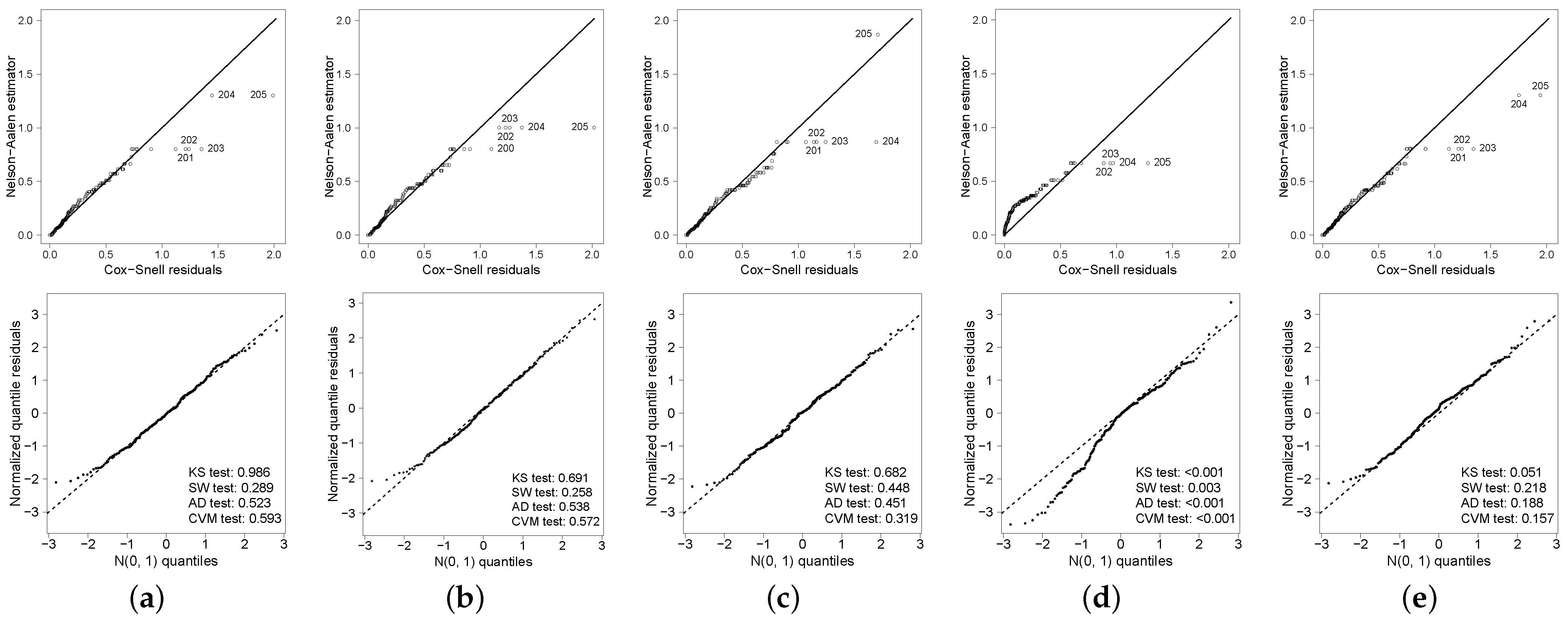
We consider the Bell cure rate model for analyzing this dataset. For comparison purposes, we also consider the Pocr, Locr, NBcr, Geocr and Bincr models. We assume the Weibull distribution for the time-to-event for the concurrent causes. First we assess the goodness of fit of the models. For such purpose, we use the Cox-Snell residual, see, e.g., [23] and the normalized quantile residual [24]. In Figure 3, we see that the Bellcr, Pocr, Locr and Geocr models yield a reasonable fit. However, the deviation from the identity line in both residuals plot is evident for the NBcr model. We omit the results for the Bincr model because the plots are similar to the ones for the NBcr model. For this reason, we disregard the NBcr and Bincr models. The Cox-Snell residuals highlight observations 200–205, which correspond to the largest censored times. On the other hand, the normalized quantile residuals do not suggest the presence of possible poorly fitted observations.

Table 6. Parameter estimates, standard errors (SE) and maximum value of the log-likelihood function $\left(\ell \left(\widehat{\mathbf{\psi }}\right)\right)$ for different models.

Parameter	Model
	Bellcr		Pocr		Locr		Geocr
	Estimate	SE	Estimate	SE	Estimate	SE	Estimate	SE
${\beta }_0$	1.8759	0.2449	1.9039	0.3431	1.6771	0.3566	1.8127	0.3501
${\beta }_1$	−1.4536	0.2843	−1.4814	0.3901	−1.4816	0.3278	−1.4807	0.3569
${\beta }_2$	−0.1908	0.0416	−0.1960	0.0705	−0.1412	0.0356	−0.1785	0.0537
$\alpha$	−3.2461	0.3124	−2.9435	0.3411	−4.1863	0.5154	−3.4907	0.3916
$\nu$	1.8287	0.1808	1.7368	0.2178	2.2110	0.2725	1.9132	0.2357
$exp\left({\beta }_1\right)$	0.2337	0.0664	0.2273	0.0887	0.2273	0.0745	0.2275	0.0812
$exp\left({\beta }_2\right)$	0.8263	0.0344	0.8220	0.0580	0.8683	0.0309	0.8365	0.0449
$\ell \left(\widehat{\mathbf{\psi }}\right)$	−206.3		−207.5		−203.7		−205.4

displays parameter estimates and odds ratio for the Bellcr, Locr, Pocr and Geocr models. At a 5% significance level, the coefficients of ulceration status $\left({\beta }_1\right)$ and tumor thickness $\left({\beta }_2\right)$ are significant and the negative sign is as expected. Moreover, the estimates of $\nu$ indicate that the exponential distribution for the latent times in Section 1 is not adequate.

Note that for all the models, $exp\left({\widehat{\beta }}_1\right)\approx 0.23$. Therefore, patients with ulceration have approximately their probability of being cured reduced by a quarter in relation with patients without ulceration.

Table 7. Vuong’s statistic and p-value when testing the Bell cure rate model against some alternatives.

Model	Pocr	Locr	Geocr
Vuong’s statistic	−2.473	1.238	1.146
p-Value	0.013	0.216	0.252

shows the Vuong’s statistic for the fitted models. At a 5% significance level, we conclude that the Bellcr model is preferred to the Pocr model. Moreover, there is no significant difference among the Bellcr and the Locr and Geocr models.

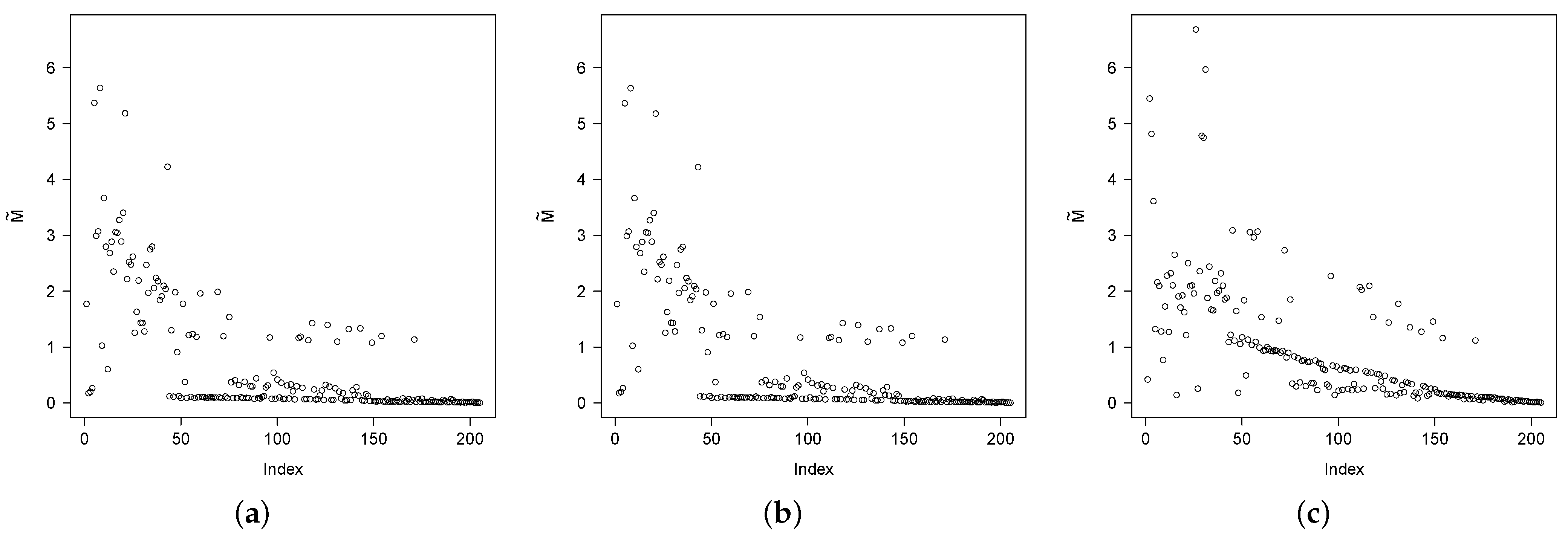
Figure 4 shows the estimates of the mean of the conditional distribution of $M_i\mid t_i,{\delta }_i;\widehat{\mathbf{\psi }}$, say ${\tilde{M}}_i$, for $i=1,\dots ,n$. As previously discussed, values closer to 0 suggest which individuals are cured. Note that the Bellcr and Locr models provide very similar values. For instance, the observation 6 corresponds to a patient who died after 204 days (0.56 years), with ulceration and a tumor thickness of 4.84 cm., providing ${\tilde{M}}_i$ equal to 2.988, 2.985 and 2.156 for Bellcr, Locr and Geocr models, respectively. Therefore, the three models suggest that this observation has a greater number of carcinogenic cells (a susceptible individual). Similarly, the observation 149 corresponds to a patient who died after 2782 days (7.62 years), without ulceration and a tumor thickness of 1.94 cm., providing ${\tilde{M}}_i$ equal to 1.076, 1.076 and 1.453 for Bellcr, Locr and Geocr models. This explains why the patient 6 fails in a time considerably lower than patient 149. In a similar way, the observation 203 has a censored time after 4688 days (12.84 years), without ulceration and a tumor thickness of 0.48 cm., resulting in ${\tilde{M}}_i$ equal to 0.002, 0.002 and 0.015 for the three models. In this case, the models agree that this patients is a potentially cured individual.

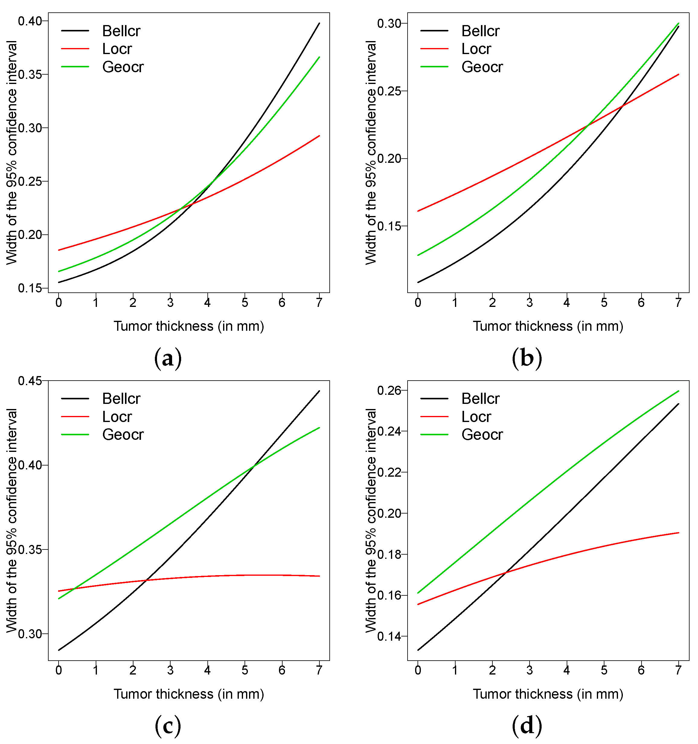
Finally, Figure 5 presents the width of the 95% confidence intervals for the conditional cure rate in (9) and Figure 6 displays estimates of cure rate under the Bellcr, Locr and Geocr models. In all models, the confidence intervals are computed using the delta method [25] (Theorem 3.4.5) using expressions of the covariance matrix of the estimators in the power series cure rate model presented in Gallardo et al. [14]. For the Locr and Geocr models, the conditional cure rate is computed as in Remark 1. Note that the Bellcr model provides more accurate confidence intervals for some settings in Figure 5. Finally, Figure 6 shows the conditional cure rate in Equation (9) for different in terms of the tumor thickness for $t_0=0$ and $t_0=5$ years and patients with and without ulceration.

6. Conclusions

In this paper, a cure rate model is proposed under the competing risks setup. For the number of competing causes of the event of interest, we posit the Bell distribution. This is a one-parameter distribution that accommodates overdispersed counts. [26] emphasized that the Poisson distribution represents a strong assumption when modelling the number of competing causes. Therefore, compared to the two-parameter negative binomial distribution, the proposed model is more parsimonious. The cure rate is a parameter linked to covariates, facilitating the comparison with other models. Parameter estimates are computed through iterative steps of the EM algorithm. In order to compare different models, the test statistic proposed in [21] is implemented. In our simulation studies, the estimation method and the test statistic have a good performance.

A dataset on melanoma is analyzed using the proposed model as well as some models from the literature. Extensions of the proposed model to accommodate other types of censoring (e.g., interval censoring) might be a theme for future work.

References

- Boag, J.W. Maximum likelihood estimates of the proportion of patients cured by cancer therapy. J. R. Stat. Soc. B 1949, 35, 15–53. [Google Scholar] [CrossRef]
- Berkson, J.; Gage, R.P. Survival curve for cancer patients following treatment. J. Am. Stat. Assoc. 1952, 47, 501–515. [Google Scholar] [CrossRef]
- Yakovlev, A.Y.; Tsodikov, A.D. Stochastic Models of Tumor Latency and Their Biostatistical Applications; World Scientific: Singapore, 1996. [Google Scholar]
- Rodrigues, J.; Cancho, V.G.; de Castro, M.; Louzada-Neto, F. On the unification of the long-term survival models. Stat. Probab. Lett. 2009, 79, 753–759. [Google Scholar] [CrossRef]
- Rodrigues, J.; de Castro, M.A.; Cancho, V.G.; Balakrishnan, N. COM-Poisson cure rate survival model and an application to a cutaneous melanoma data. J. Stat. Plan. Inference 2009, 139, 3605–3611. [Google Scholar] [CrossRef]
- Cancho, V.G.; Louzada, F.; Ortega, E.M. The power series cure rate model: An application to a cutaneous melanoma data. Commun. Stat. Simul. Comput. 2013, 42, 586–602. [Google Scholar] [CrossRef]
- Gallardo, D.I.; Gómez, H.W.; Bolfarine, H. A new cure rate model based on the Yule-Simon distribution with application to a melanoma data set. J. Appl. Stat. 2017, 44, 1153–1164. [Google Scholar] [CrossRef]
- Gallardo, D.I.; Gómez, Y.M.; De Castro, M. A flexible cure rate model based on the polylogarithm distribution. J. Stat. Comput. Simul. 2018, 88, 2137–2149. [Google Scholar] [CrossRef]
- Gallardo, D.I.; Gómez, Y.M.; Gómez, H.W.; De Castro, M. On the use of the modified power series family of distributions in a cure rate model context. Stat. Methods Med. Res. 2020, 29, 1831–1845. [Google Scholar] [CrossRef] [PubMed]
- Cancho, V.G.; Macera, M.A.C.; Suzuki, A.K.; Louzada, F.; Zavaleta, K.E.C. A new long-term survival model with dispersion induced by discrete frailty. Lifetime Data Anal. 2020, 26, 221–244. [Google Scholar] [CrossRef]
- Leao, J.; Bourguignon, M.; Gallardo, D.I.; Rocha, R.; Tomazella, V. A new cure rate model with flexible competing causes with applications to melanoma and transplantation data. Stat. Med. 2020, 24, 3272–3284. [Google Scholar] [CrossRef] [PubMed]
- Castellares, F.; Lemonte, A.J.; Santos, M.A.C. On the Nielsen distribution. Braz. J. Probab. Stat. 2020, 1, 90–111. [Google Scholar] [CrossRef]
- Noack, A. A class of random variables with discrete distributions. Ann. Math. Stat. 1950, 21, 127–132. [Google Scholar] [CrossRef]
- Gallardo, D.I.; Romeo, J.S.; Meyer, R. A simplified estimation procedure based on the EM algorithm for the power series cure rate model. Commun. Stat. Simul. Comput. 2017, 46, 6342–6359. [Google Scholar] [CrossRef]
- Tsodikov, A.D.; Ibrahim, J.G.; Yakovlev, A.Y. Estimating cure rates from survival data: An alternative to two-component mixture models. J. Am. Stat. Assoc. 2003, 98, 1063–1078. [Google Scholar] [CrossRef] [PubMed] [Green Version]
- Cancho, V.G.; De Castro, M.; Dey, D.K. Long-term survival models with latent activation under a flexible family of distributions. Braz. J. Probab. Stat. 2013, 27, 585–600. [Google Scholar] [CrossRef]
- Chen, M.-H.; Ibrahim, J.G.; Sinha, D. A new Bayesian model for survival data with a surviving fraction. J. Am. Stat. Assoc. 1999, 94, 909–919. [Google Scholar] [CrossRef]
- Corless, R.M.; Gonnet, G.H.; Hare, D.E.G.; Jeffrey, D.J.; Knuth, D.E. On the Lambert W function. Adv. Comput. Math. 1996, 5, 329–359. [Google Scholar] [CrossRef]
- R Development Core Team. A Language and Environment for Statistical Computing; R Foundation for Statistical Computing: Vienna, Austria, 2021. [Google Scholar]
- Gilbert, P.; Varadhan, R. numDeriv: Accurate Numerical Derivatives, R Package Version; Available online: http://optimizer.r-forge.r-project.org/ (accessed on 3 July 2021).
- Vuong, Q.H. Likelihood Ratio Tests for Model Selection and non-nested Hypotheses. Econometrica 1989, 57, 307–333. [Google Scholar] [CrossRef] [Green Version]
- Scheike, T.H.; Zhang, M.J. Analyzing competing risk data using the R timereg package. J. Stat. Softw. 2011, 38, 1–15. [Google Scholar] [CrossRef] [Green Version]
- Conlon, A.S.C.; Taylor, J.M.G.; Sargent, D.J. Multi-state models for colon cancer recurrence and death with a cure fraction. Stat. Med. 2014, 33, 1750–1766. [Google Scholar] [CrossRef] [Green Version]
- Dunn, P.K.; Smyth, G.K. Randomized quantile residuals. J. Comput. Graph. Stat. 1996, 5, 236–244. [Google Scholar]
- Sen, P.K.; Singer, J.M. Large Sample Methods in Statistics: An Introduction with Applications; Chapman & Hall: New York, NY, USA, 1993. [Google Scholar]
- Tournoud, M.; Ecochard, R. Promotion time models with time-changing exposure and heterogeneity: Application to infectious diseases. Biom. J. 2008, 50, 395–407. [Google Scholar] [CrossRef] [PubMed]
Figure 1.
Variance of the number of competing causes as a function of the cure rate for some models.
Figure 2.
Scheme to draw the covariates in the simulation study. Bern (0.5) denotes the Bernoulli distribution with probability 0.5 and denotes the uniform distribution on ).
Figure 3.
Cox-Snell residuals (upper panels) and normalized quantile residuals plots (lower panels): (a) Bellcr, (b) Pocr, (c) Locr, (d) NBcr and (e) Geocr models.
Figure 4.
Estimate of the mean of the conditional distribution of in melanoma data set using (a) Bellcr, (b) Locr and (c) Geocr models.
Figure 5.
Width of the 95% confidence interval for the conditional cure rate: (a) without ulceration and year, (b) without ulceration and years, (c) with ulceration and years and (d) with ulceration and years.
Figure 6.
Estimates of the conditional cure rate ( in Equation (9)) for years: (a) without ulceration and (b) with ulceration. Estimated survival function for a tumor thickness of 10 cms: (c) without ulceration and (d) with ulceration.