
An Extension of the Truncated-Exponential Skew- Normal Distribution
by
 , , and
Pilar A. Rivera
1, 
Diego I. Gallardo
2,
Osvaldo Venegas
3,*,
Marcelo Bourguignon
4 and
Héctor W. Gómez
1 1
Departamento de Matemáticas, Facultad de Ciencias Básicas, Universidad de Antofagasta, Antofagasta 1240000, Chile
2
Departamento de Matemática, Facultad de Ingeniería, Universidad de Atacama, Copiapó 1530000, Chile
3
Departamento de Ciencias Matemáticas y Físicas, Facultad de Ingeniería, Universidad Católica de Temuco, Temuco 4780000, Chile
4
Departamento de Estatística, Universidade Federal do Rio Grande do Norte, Natal 59078-970, Brazil
*
Author to whom correspondence should be addressed.
Mathematics 2021, 9(16), 1894; https://doi.org/10.3390/math9161894
Submission received: 24 June 2021
/
Revised: 15 July 2021
/
Accepted: 27 July 2021
/
Published: 9 August 2021
(This article belongs to the Section Probability and Statistics)
Abstract
:In the paper, we present an extension of the truncated-exponential skew-normal (TESN) distribution. This distribution is defined as the quotient of two independent random variables whose distributions are the TESN distribution and the beta distribution with shape parameters q and 1, respectively. The resulting distribution has a more flexible coefficient of kurtosis. We studied the general probability density function (pdf) of this distribution, its survival and hazard functions, some of its properties, moments and inference by the maximum likelihood method. We carried out a simulation and applied the methodology to a real dataset.
1. Introduction
The Slash (S) distribution is a generalization of the normal model. Its stochastic representation is given by
where is independent of and .
represents the canonical Slash model and the standard normal model is obtained for . The pdf of the canonical S distribution is
where represents the pdf of the standard normal model (see Johnson et al. [1]). This distribution is characterized by having heavier tails than normal distribution, i.e., it has greater kurtosis.
Properties of the S distribution are discussed by Rogers and Tukey [2] and Mosteller and Tukey [3]. The ML parameters for location and scale in the S model are discussed in Kadafar [4]. Wang et al. [5] studied a multivariate version of the S distribution and a multivariate skew version. Gómez et al. [6] extended the S distribution using the family of univariate and multivariate elliptical distributions also was extended by using the S model in Gómez et al. [7].
Nadarajah et al. [8] proposed the idea of constructing biased distributions, motivated by Azzalini [9], including asymmetry in these. A unified approach for the construction of models of this kind is given in Ferreira and Steel [10]. If X is a symmetrical random variable around zero with pdf and cumulative distribution function (cdf) , the new random variable Y is defined with pdf given by:
with denoting a pdf in the interval . Then Y is a skew version of the variable X. The most commonly-used versions of (2) are the skew distributions proposed by Azzalini [9] in the form:
The skew-normal (SN) model is obtained as a particular case of (3) considering and , where denotes the cdf of the standard normal model.
In the present paper, we extend the TESN model introduced by Nadarajah et al. [8], based on the Slash methodology. The pdf of the TESN distribution is given by:
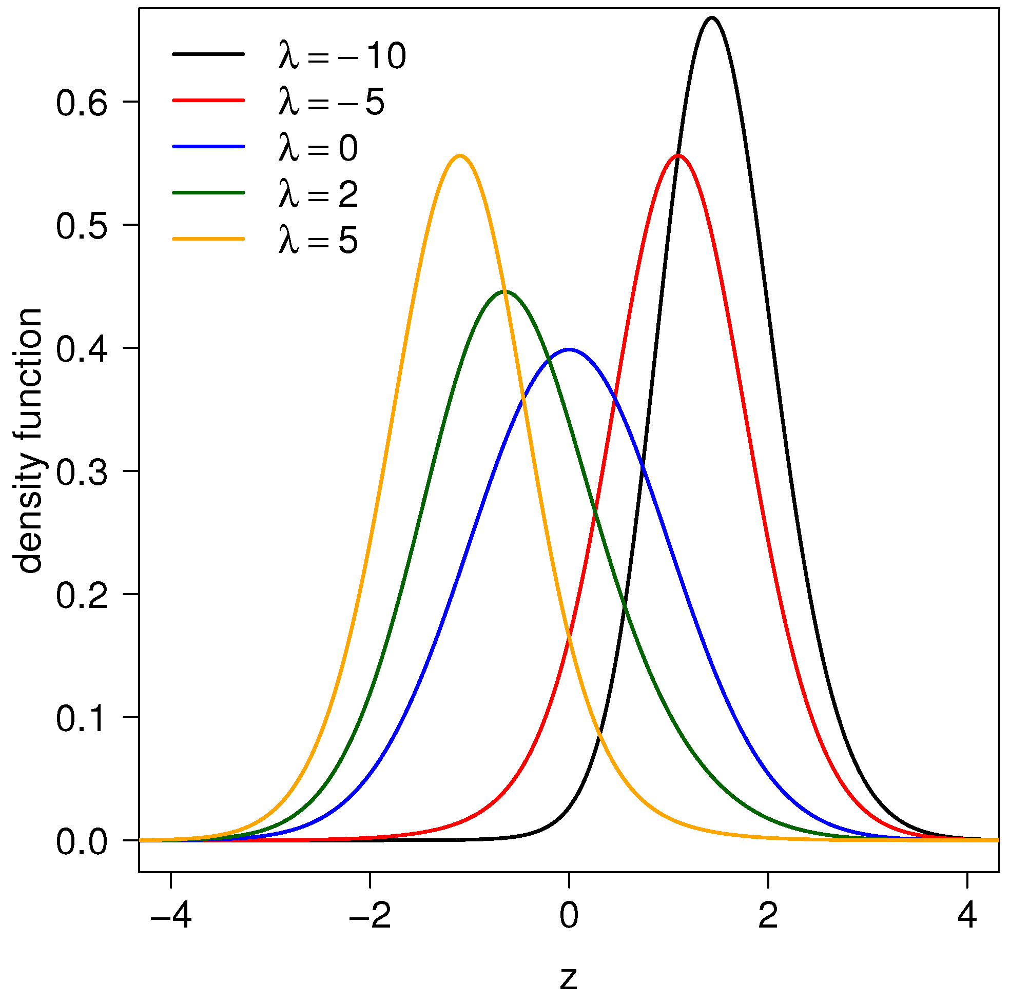
where . Hereafter, we use the notation to indicate that X is a random variable following a TESN distribution. According to Barreto-Souza and Simas [11], the distribution presents different behavior for a large , suggesting that this is a rich class of distributions. Furthermore, the parameter can be interpreted as a concentration parameter. Figure 1 shows the graph of the TESN pdf function with variations of the parameter .
The extension of this model is based on the quotient of two independent random variables, with TESN distribution and a power of the uniform distribution , respectively, obtaining a distribution with a more flexible coefficient of kurtosis and so generating an appropriate model for fitting data. In practical terms, this generalization is based on the search for distributions that are more flexible, which may provide a “better fit” than the TESN distribution. For example, see the works by Gomes et al. [12], Maurya and Nadarajah [13] and the references therein.
The article is organized as follows. In Section 2 we study the representation, pdf, properties, and graphs. In Section 3, we present a Monte Carlo simulation experiment to evaluate the maximum likelihood estimates of the model parameters in Section 2. In Section 4, we provide an application of the proposed distribution. In Section 5, we conclude with some final comments.
2. Incorporating Kurtosis
In this section, we introduce a new extension of the TESN distribution. We studied its pdf, survival and hazard functions, moments, location and scale parameters, and their log-likelihood equations.
2.1. Representation
Following the representation of the Slash distribution, the representation of this new distribution is given by the following definition:
Definition 1.
A random variable (r.v.) Z has a Slashed Truncated Exponential Skew-Normal (STESN) distribution, denoted by if it is represented by:
where and are independent variables, , .
2.2. Probability Density Function
The following proposition shows the pdf function for the STESN distribution, generated using the stochastic representation given in (5) and using the Jacobian method for transforming the r.v.:
Proposition 1.
If the pdf of Z is given by:
where , , and .
Proof.
The pdf is generated using the representation given in (5). Using the Jacobian method for transforming the r.v. we obtain ; , calculating the Jacobian, we obtain:
replacing the joint pdf :
where , , and . Hence, marginalizing with respect to variable W, we obtain:
where , , and:
□
Proposition 2.
Let . If the r.v. Z converges in law to the r.v. .
Proof.
Remark 1.
The above proposition implies that if then the pdf of the STESN distribution approaches the pdf of a TESN distribution.
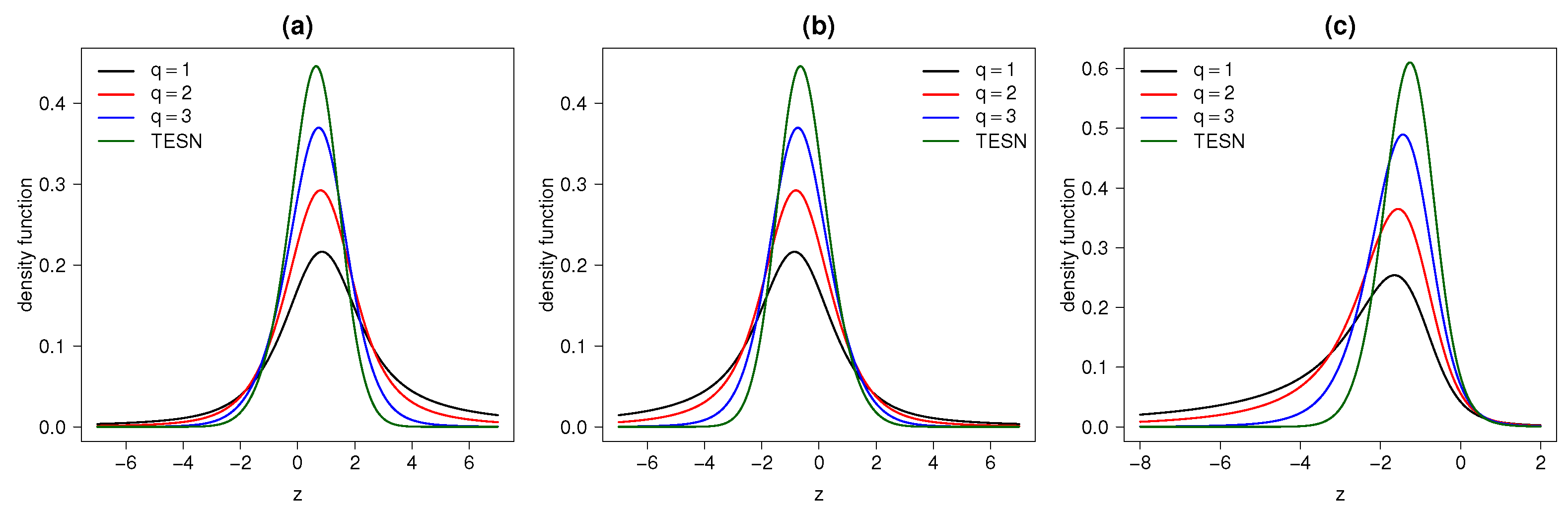
Figure 2a,b show the graphs for the pdf of this model for some parameter values.
2.3. Reliability Analysis
For the study of failure times, we need to consider a time y, where we have . Therefore, in our model we study the case of non-negative variables where , thus, the model must be transformed to obtain the following pdf:
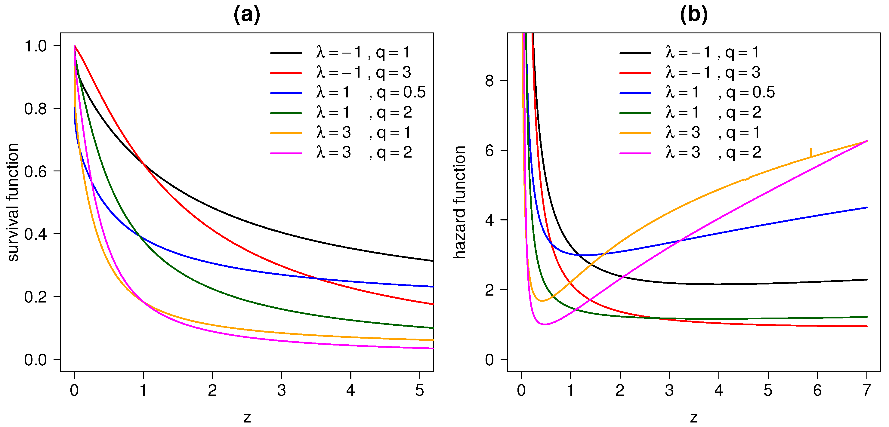
where , , , and . Figure 2c shows the graphs of the pdf for different parameter values. Once the transformation is complete, we obtain the survival and hazard functions. The survival function is defined as the probability that a subject does not experience the event of interest before a moment t, and in our model is given by:
where . It also gives the hazard function defined as the probability of failure during a time interval given in our model by:
where . Figure 3a,b show the graphs of survival and hazard functions respectively, for different parameter values.
2.4. Moments
Let Z be a r.v. where , the r-th moment for the variable is given by the following proposition.
Proposition 3.
Using the representation (5), the r-th moment of the r.v. Z is:
where and the k-th order statistic of a random variable with distribution .
Proof.
The r-th moments of Z can be calculated as:
where is the r-th moment for the model proposed by Nadarajah et al. [8] given by:
where the k-th order statistic of a random variable with distribution and the r-th moment of the r.v. .
Therefore the r-th moment for the variable is given by:
□
Using this proposition, the first four moments of the r.v. Z are given in the following corollary.
Corollary 1.
From the -th moment of the r.v. represented by (10), we obtain the first four moments of the variable, given by:
2.5. Incorporation of Parameters
To produce a more flexible distribution, we will extend this model to location and scale parameters as , where obtaining the following proposition.
Proposition 4.
2.6. Log Likelihood Equations
Let be a random sample of the r.v. X with distribution, the log-likelihood function can be written as:
where and .
For each parameter we have the following likelihood equations:
where . Furthermore, , , , and .
As can be observed, this system can only be resolved by iterative procedures such as Newton–Raphson. As an alternative, it is also possible is to use the optim routine implemented in R software [15]. Standard errors for parameters can be estimated using the hessian matrix of the log-likelihood function, which can be estimated, for instance, using the pracma package (see Borchers [16]).
2.7. STESN or TESN Model?
In order to decide between the STESN and TESN models, we can use the traditional Akaike (AIC, Akaike [17]) and Schwarz (BIC, Schwartz [18]) criteria. As the TESN model corresponds to the STESN model with , we can use the likelihood ratio test (LRT) to decide between the two models considering (TESN model) versus (STENS model). This is a problem where the null hypothesis is exactly on the boundary of the parameter space. This kind of problem was first discussed in Chernoff [19]. This problem is also presented, for instance, in a random effects model when we are interested in testing if the variance of such random effects is zero (see Stram and Lee [20] and Gallardo et al. [21]) or in a cure rate model when we are interested in testing the presence of cured individuals in the population (see Maller and Zhou [22]). In this particular case, the statistic for the LRT, say , does not converge asymptotically to the usual distribution, i.e., the chi-squared distribution with 1 degree of freedom, but converges to , i.e., a 50-50 mixture between a point mass in 0 and distribution.
3. Simulation Study
In this section, we will study the behavior of ML estimators in finite samples, verifying empirically whether these estimators have desirable properties (unbiased, asymptotically efficient, verification of the normal asymptotic distribution of ML estimators).
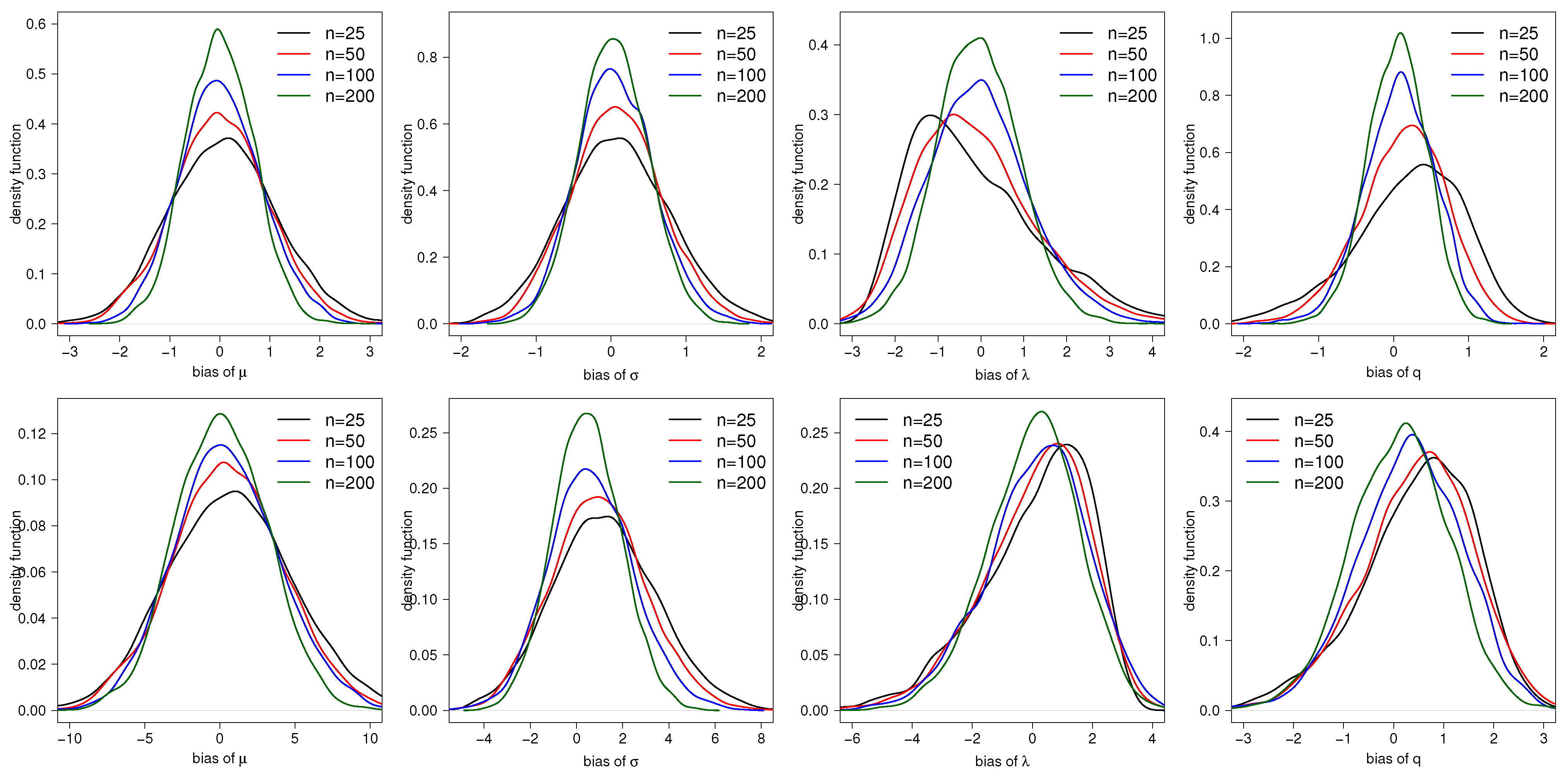
The random variables of the TESN distribution and the Beta distribution were generated to obtain our new variable with pdf shown in (15). The initial values used for optimization were obtained by a sequence of values which maximized this function. In this sequence, takes values between and 3, q between 1 and 5, between and 2, and between 2 and 10. This process was repeated 5000 times with sample size , , and 200 for different combinations of parameters. Table 1 presents the empirical bias, the standard errors (SE), root of the mean squared error (RMSE), and 95% coverage probabilities (CP) for the estimators of the parameters of the STESN distribution with different combinations of parameters and sample sizes. From those tables, notice that the biases SE and RMSE decrease as the sample size increases, suggesting that estimators are consistent. Furthermore, the asymptotic confidence intervals have an empirical CP differing from the nominal values, especially when the sample size is small. However, we observe that the asymptotic confidence intervals converge to the nominal values when the sample size is increased. Figure 4 shows the estimated pdf for the ML estimators of , and q for two combinations of parameters, showing graphically that the skewness of the estimators disappears progressively when the sample sizes increases. We also note that the distribution of the estimators for and q are more asymmetric than the distribution of the estimators for and , especially in small sample sizes.
4. Application to a Data Set
In this section, we will present a real data application to illustrate the STESN model compared with other models discussed in the literature. These data were presented by Barlow et al. [23] and represent the fatigue fracture life of Kevlar 373/epoxi subjected to a constant pressure of stress until they all fail. To obtain the parameter estimations, the optim command was used and its estimation errors were calculated by the Hessian matrix, both in R software. Codes are available as supplementary material.
Table 2 shows a summary of the dataset, including the sample size n, the mean , the standard deviation S, the asymmetry coefficient , the kurtosis coefficient , the minimum , and the maximum . A high kurtosis value is observed.
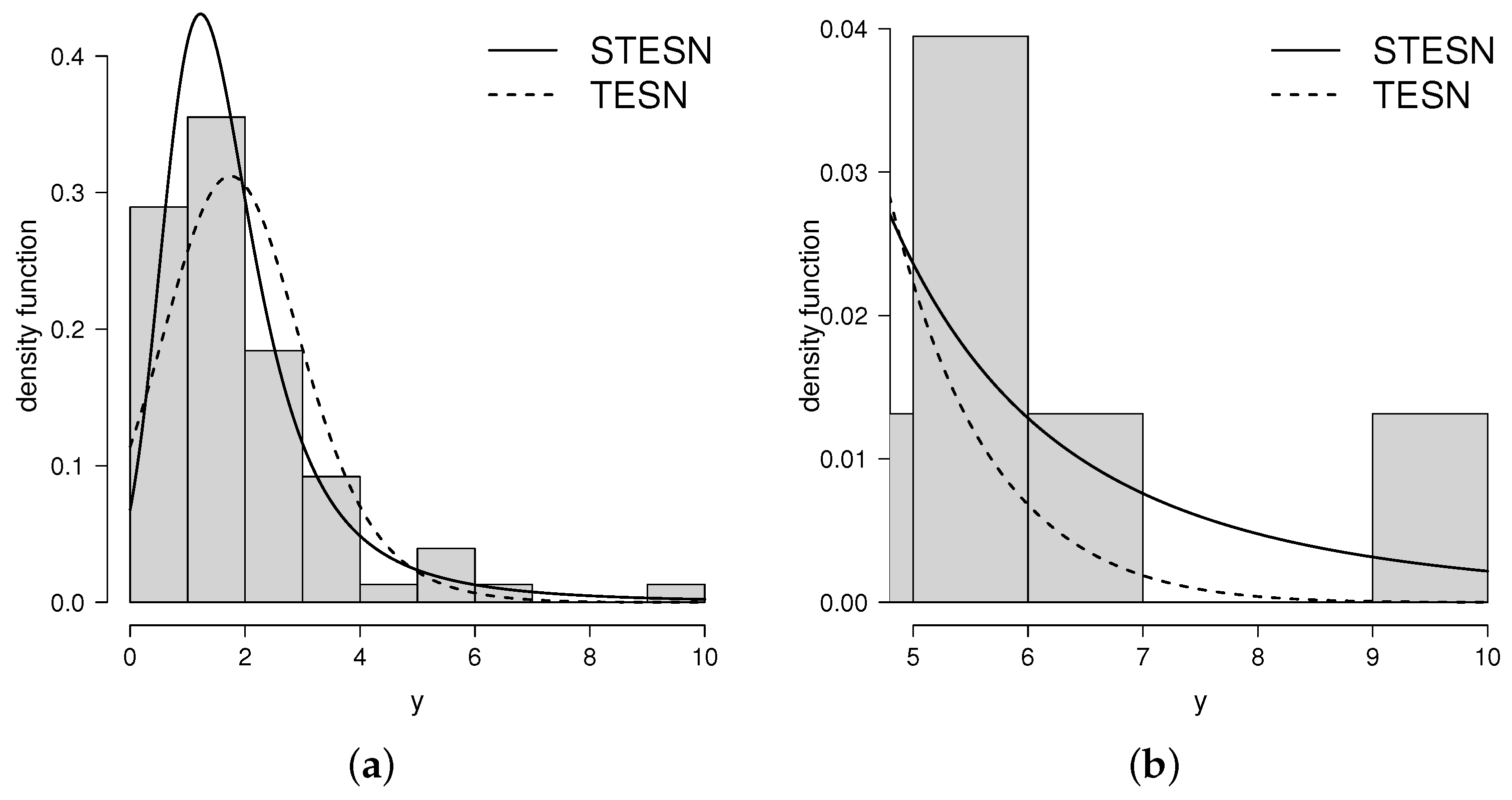
Table 3 shows the results of the fit; the TESN distribution was compared with the STESN distribution by AIC and BIC criteria. It is concluded that the distribution which achieves the best fit for this dataset is the STESN distribution, since it presents a lower value in the criteria. Furthermore, Table 3 provides the Kolmogorov–Smirnov statistic (KSS), a formal goodness-of-fit test to verify which distribution gives a better fit for these data. Small values of this statistic suggests a better fit. Thus, according to the Kolmogorov–Smirnov test, the STESN model fits the current data better than the TESN model.
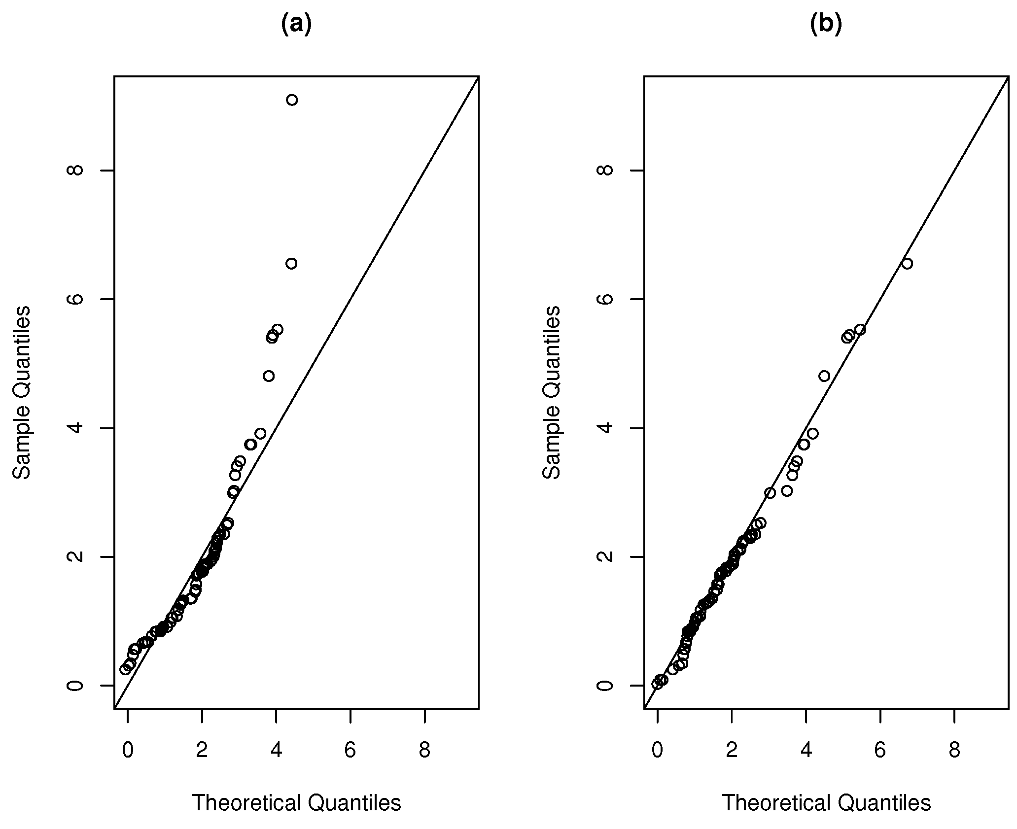
Figure 5a,b present a histogram of the data with the densities fitted for the data set and Figure 6a,b present the QQ-plot of the densities fitted for the dataset, showing the good fit given by the new distribution.
In our problem, the observed statistic for the LRT to decide between the TESN and STESN models, discussed in Section 2.7, is with an associated p-value . Therefore, the is rejected under any usual level of significance and the STESN model is preferred over the TESN model.
5. Final Comments
In this paper, we introduced an extension of the TESN distribution from which we obtained a distribution that showed greater flexibility in the coefficient of kurtosis. Some mathematical properties of the new distribution were studied. Note that the formulae derived easily implemented in different softwares. Inference was implemented based on the ML approach, and its performance was assessed by Monte Carlo simulations using R software. An application to a real dataset showed that the new model produced a better fit than the TESN model. This application demonstrated the practical importance of the new model, and also showed the advantage of STESN over TESN. We hope this new distribution may attract wider applications.
Supplementary Materials
The following are available online at https://www.mdpi.com/article/10.3390/math9161894/s1.
Author Contributions
Conceptualization, P.A.R. and D.I.G.; methodology, H.W.G.; software, D.I.G.; validation, P.A.R., D.I.G., and H.W.G.; formal analysis, O.V.; investigation, O.V. and M.B.; writing—original draft preparation, P.A.R.; writing—review and editing, O.V. and M.B.; funding acquisition, M.B. All authors contributed equally to this work. All authors have read and agreed to the published version of the manuscript.
Funding
The research of Pilar A. Rivera and Héctor W. Gómez was supported by SEMILLERO UA-2021 (Chile). The research of O. Venegas was supported by Vicerrectoría de Investigación y Postgrado of the Universidad Católica de Temuco, Projecto interno FEQUIP 2019-INRN-03.
Institutional Review Board Statement
Not applicable.
Informed Consent Statement
Not applicable.
Data Availability Statement
The data used in Section 4 can be obtained from the corresponding reference.
Conflicts of Interest
The authors declare no conflict of interest.
References
- Johnson, N.L.; Kotz, S.; Balakrishnan, N. Continuous Univariate Distributions, 2nd ed.; Wiley Series in Probability and Statistics; Wiley: New York, NY, USA, 1995. [Google Scholar]
- Rogers, W.H.; Tukey, J.W. Understanding some long-tailed symmetrical distributions. Stat. Neerl. 1972, 26, 211–226. [Google Scholar] [CrossRef]
- Mosteller, F.; Tukey, J.W. Data Analysis and Regression: A Second Course in Statistics; Addison-Wesley: Reading, MA, USA, 1977. [Google Scholar]
- Kadafar, K. A biweight approach to the one-sample problem. J. Am. Stat. Assoc. 1982, 77, 416–424. [Google Scholar] [CrossRef]
- Wang, J.; Boyer, J.; Genton, M.G. A skew-symmetric representation of multivariate distributions. Stat. Sin. 2004, 14, 1259–1270. [Google Scholar]
- Gómez, H.W.; Quintana, F.A.; Torres, F.J. New family of slash-distributions with elliptical contours. Stat. Probab. Lett. 2007, 77, 717–725. [Google Scholar] [CrossRef]
- Gómez, H.W.; Olivares-Pacheco, J.F.; Bolfarine, H. An extension of the generalized Birnbaum-Saunders distribution. Stat. Probab. Lett. 2009, 79, 331–338. [Google Scholar] [CrossRef]
- Nadarajah, S.; Nassiri, V.; Mohammadpour, A. Truncated-exponential skew-symmetric distributions. Statistics 2014, 48, 872–895. [Google Scholar] [CrossRef]
- Azzalini, A. A Class of Distributions Which Includes the Normal Ones. Scand. J. Stat. 1985, 12, 171–178. [Google Scholar]
- Ferreira, J.T.A.S.; Steel, M.F.J. A constructive representation of univariate skewed distributions. J. Am. Stat. Assoc. 2006, 101, 823–829. [Google Scholar] [CrossRef] [Green Version]
- Barreto-Souza, W.; Simas, A.B. The exp- G family of probability distributions. Braz. J. Probab. Stat. 2013, 27, 84–109. [Google Scholar] [CrossRef]
- Gomes, A.E.; Da-Silva, C.Q.; Cordeiro, G.M. The Exponentiated G Poisson Model. Commun. Stat.-Theory Methods 2015, 44, 4217–4240. [Google Scholar] [CrossRef]
- Maurya, S.K.; Nadarajah, S. Poisson Generated Family of Distributions: A Review. Sankhya B 2020, 1–57. [Google Scholar] [CrossRef]
- Lehmann, E.L. Elements of Large-Sample Theory; Springer: New York, NY, USA, 1999. [Google Scholar]
- R Development Core Team. A Language and Environment for Statistical Computing; R Foundation for Statistical Computing: Vienna, Austria, 2021. [Google Scholar]
- Borchers, H.W. Pracma: Practical Numerical Math Functions, R package version 2.3.3; 2021. Available online: https://CRAN.R-project.org/package=pracma (accessed on 24 June 2021).
- Akaike, H. A new look at the statistical model identification. IEEE Trans. Automat. Contr. 1974, 19, 716–723. [Google Scholar] [CrossRef]
- Schwarz, G. Estimating the dimension of a model. Ann. Stat. 1978, 6, 461–464. [Google Scholar] [CrossRef]
- Chernoff, H. On the distribution of the likelihood ratio. Ann. Stat. 1954, 54, 573–578. [Google Scholar] [CrossRef]
- Stram, D.O.; Lee, J.W. Variance components testing in the longitudinal mixed effects model. Biometrics 1994, 50, 1171–1177. [Google Scholar] [CrossRef] [PubMed]
- Gallardo, D.I.; Bolfarine, H.; Pedroso-de-Lima, A.C. A clustering cure rate model with application to a sealant study. J. Appl. Stat. 2017, 44, 2949–2962. [Google Scholar] [CrossRef]
- Maller, R.; Zhou, S. Testing for the Presence of Immune or Cured Individuals in Censored Survival Data. Biometrics 1995, 51, 1197–1205. [Google Scholar] [CrossRef] [PubMed]
- Barlow, R.E.; Toland, R.H.; Freeman, T. A Bayesian analysis of stress rupture life of Kevlar 49/epoxy spherical pressure vessels. In Procedings Conference on Applications of Statistics; Marcel Dekker: New York, NY, USA, 1984. [Google Scholar]
Figure 1.
TESN pdf for different values of .

Figure 2.
STESN for values of (a) ; (b) ; and (c) for different values of q.

Figure 3.
(a) Survival function and (b) hazard function for log-STESN model with different combinations of values for and q.
Figure 3.
(a) Survival function and (b) hazard function for log-STESN model with different combinations of values for and q.

Figure 4.
Estimated pdf for the ML estimators of , and q in the TESN distribution for: (upper panels), and (lower panels).
Figure 4.
Estimated pdf for the ML estimators of , and q in the TESN distribution for: (upper panels), and (lower panels).

Figure 5.
Estimated pdf for STESN and TESN for kevlar data set (a) and a zoom for the right tail (b).
Figure 5.
Estimated pdf for STESN and TESN for kevlar data set (a) and a zoom for the right tail (b).

Figure 6.
QQ-plot for the (a) TESN and (b) STESN distributions for the dataset.


Table 1.
Empirical bias, SE, RMSE, and 95% CP for the ML estimators of , , , and q with different combinations of parameters and sample sizes.
Table 1.
Empirical bias, SE, RMSE, and 95% CP for the ML estimators of , , , and q with different combinations of parameters and sample sizes.
| True Values | ||||||||||||||||||||
|---|---|---|---|---|---|---|---|---|---|---|---|---|---|---|---|---|---|---|---|---|
| q | bias | SE | RMSE | CP | bias | SE | RMSE | CP | bias | SE | RMSE | CP | bias | SE | RMSE | CP | ||||
| 0 | 1 | −3 | 1 | 0.053 | 1.140 | 1.141 | 0.903 | 0.031 | 0.882 | 0.885 | 0.909 | 0.013 | 0.662 | 0.675 | 0.912 | 0.009 | 0.449 | 0.458 | 0.939 | |
| 0.084 | 0.489 | 0.496 | 0.972 | 0.069 | 0.367 | 0.373 | 0.965 | 0.052 | 0.278 | 0.287 | 0.961 | 0.042 | 0.197 | 0.203 | 0.959 | |||||
| −0.176 | 2.336 | 2.336 | 0.887 | −0.093 | 1.914 | 1.936 | 0.892 | −0.053 | 1.366 | 1.398 | 0.906 | −0.042 | 0.892 | 0.910 | 0.921 | |||||
| q | 0.195 | 0.587 | 0.618 | 0.973 | 0.119 | 0.350 | 0.370 | 0.972 | 0.082 | 0.220 | 0.235 | 0.965 | 0.057 | 0.151 | 0.161 | 0.961 | ||||
| 0 | 1 | −1 | 1 | −0.099 | 1.473 | 1.473 | 0.918 | −0.078 | 1.045 | 1.049 | 0.928 | −0.051 | 0.704 | 0.711 | 0.935 | −0.033 | 0.473 | 0.477 | 0.948 | |
| 0.159 | 0.532 | 0.555 | 0.970 | 0.111 | 0.372 | 0.388 | 0.965 | 0.075 | 0.252 | 0.263 | 0.958 | 0.044 | 0.179 | 0.184 | 0.953 | |||||
| −0.154 | 2.398 | 2.399 | 0.887 | −0.117 | 1.810 | 1.822 | 0.889 | −0.083 | 1.183 | 1.196 | 0.907 | −0.060 | 0.765 | 0.770 | 0.915 | |||||
| q | 0.214 | 0.555 | 0.594 | 0.962 | 0.163 | 0.479 | 0.506 | 0.960 | 0.080 | 0.229 | 0.243 | 0.958 | 0.041 | 0.147 | 0.152 | 0.953 | ||||
| 0 | 1 | 3 | 1 | −0.100 | 1.166 | 1.170 | 0.901 | −0.091 | 0.907 | 0.913 | 0.928 | −0.077 | 0.615 | 0.624 | 0.936 | −0.047 | 0.448 | 0.458 | 0.945 | |
| 0.094 | 0.512 | 0.514 | 0.974 | 0.076 | 0.394 | 0.401 | 0.968 | 0.056 | 0.254 | 0.261 | 0.961 | 0.053 | 0.194 | 0.201 | 0.957 | |||||
| 0.251 | 2.300 | 2.299 | 0.871 | 0.192 | 1.843 | 1.875 | 0.896 | 0.167 | 1.295 | 1.322 | 0.917 | 0.094 | 0.864 | 0.887 | 0.925 | |||||
| q | 0.168 | 0.657 | 0.678 | 0.965 | 0.115 | 0.376 | 0.393 | 0.961 | 0.071 | 0.220 | 0.231 | 0.960 | 0.045 | 0.148 | 0.154 | 0.959 | ||||
| 0 | 1 | −2 | 2 | −0.061 | 1.140 | 1.139 | 0.905 | −0.033 | 1.097 | 1.097 | 0.918 | −0.031 | 0.941 | 0.950 | 0.929 | −0.010 | 0.664 | 0.672 | 0.932 | |
| 0.053 | 0.386 | 0.389 | 0.986 | 0.042 | 0.343 | 0.357 | 0.979 | 0.034 | 0.297 | 0.318 | 0.971 | 0.025 | 0.189 | 0.200 | 0.964 | |||||
| −0.192 | 2.875 | 2.880 | 0.894 | −0.151 | 2.778 | 2.783 | 0.901 | −0.122 | 2.318 | 2.355 | 0.915 | −0.097 | 1.625 | 1.652 | 0.921 | |||||
| q | 0.362 | 1.301 | 1.350 | 0.971 | 0.278 | 1.254 | 1.341 | 0.969 | 0.226 | 1.008 | 1.094 | 0.963 | 0.180 | 0.510 | 0.541 | 0.959 | ||||
| 0 | 1 | 3 | 2 | −0.205 | 1.004 | 1.024 | 0.899 | −0.079 | 0.915 | 0.918 | 0.910 | −0.061 | 0.758 | 0.762 | 0.928 | −0.044 | 0.580 | 0.581 | 0.936 | |
| 0.079 | 0.389 | 0.389 | 0.971 | 0.053 | 0.313 | 0.314 | 0.968 | 0.041 | 0.264 | 0.271 | 0.961 | 0.030 | 0.201 | 0.205 | 0.959 | |||||
| 0.278 | 2.655 | 2.668 | 0.896 | 0.212 | 2.570 | 2.569 | 0.906 | 0.144 | 2.100 | 2.127 | 0.917 | 0.100 | 1.566 | 1.578 | 0.929 | |||||
| q | 0.213 | 1.256 | 1.273 | 0.965 | 0.192 | 1.035 | 1.075 | 0.961 | 0.119 | 0.880 | 0.926 | 0.959 | 0.099 | 0.507 | 0.529 | 0.958 | ||||
| 0 | 1 | 2 | 2 | 0.164 | 1.171 | 1.191 | 0.904 | 0.115 | 1.114 | 1.115 | 0.912 | 0.079 | 0.901 | 0.904 | 0.939 | 0.052 | 0.689 | 0.693 | 0.945 | |
| 0.099 | 0.369 | 0.369 | 0.986 | 0.082 | 0.335 | 0.350 | 0.982 | 0.074 | 0.280 | 0.299 | 0.971 | 0.040 | 0.204 | 0.215 | 0.960 | |||||
| 0.381 | 3.081 | 3.103 | 0.866 | 0.242 | 2.772 | 2.782 | 0.899 | 0.171 | 2.252 | 2.267 | 0.919 | 0.127 | 1.668 | 1.683 | 0.935 | |||||
| q | 0.280 | 1.318 | 1.347 | 0.976 | 0.223 | 1.137 | 1.213 | 0.973 | 0.112 | 1.023 | 1.103 | 0.967 | 0.087 | 0.583 | 0.629 | 0.959 | ||||
| 0 | 1 | −1 | 3 | 0.023 | 1.102 | 1.102 | 0.919 | 0.022 | 1.059 | 1.059 | 0.932 | 0.005 | 1.013 | 1.013 | 0.938 | 0.004 | 0.913 | 0.914 | 0.941 | |
| 0.102 | 0.321 | 0.321 | 0.979 | 0.071 | 0.246 | 0.256 | 0.975 | 0.068 | 0.222 | 0.251 | 0.971 | 0.057 | 0.191 | 0.224 | 0.961 | |||||
| −0.134 | 3.189 | 3.188 | 0.972 | −0.116 | 3.001 | 3.002 | 0.965 | −0.072 | 2.726 | 2.725 | 0.961 | −0.049 | 2.414 | 2.417 | 0.955 | |||||
| q | 0.386 | 1.835 | 1.837 | 0.974 | 0.320 | 1.526 | 1.582 | 0.970 | 0.202 | 1.420 | 1.484 | 0.965 | 0.170 | 1.258 | 1.244 | 0.961 | ||||
| 0 | 1 | 2 | 3 | 0.128 | 1.014 | 1.022 | 0.899 | 0.069 | 0.930 | 0.930 | 0.912 | 0.061 | 0.830 | 0.832 | 0.943 | 0.046 | 0.813 | 0.815 | 0.944 | |
| 0.134 | 0.324 | 0.325 | 0.984 | 0.079 | 0.274 | 0.278 | 0.977 | 0.052 | 0.246 | 0.266 | 0.962 | 0.049 | 0.209 | 0.227 | 0.959 | |||||
| 0.159 | 2.939 | 2.942 | 0.888 | 0.128 | 2.739 | 2.752 | 0.911 | 0.116 | 2.643 | 2.655 | 0.927 | 0.082 | 2.253 | 2.264 | 0.935 | |||||
| q | 0.322 | 1.556 | 1.556 | 0.981 | 0.262 | 1.411 | 1.475 | 0.972 | 0.174 | 1.271 | 1.237 | 0.961 | 0.054 | 1.027 | 1.039 | 0.958 | ||||
| −5 | 4 | −2 | 2 | −0.354 | 4.484 | 4.495 | 0.900 | −0.225 | 4.405 | 4.405 | 0.917 | −0.137 | 3.562 | 3.600 | 0.927 | −0.040 | 2.641 | 2.670 | 0.935 | |
| 0.317 | 1.550 | 1.553 | 0.970 | 0.281 | 1.311 | 1.365 | 0.964 | 0.237 | 1.070 | 1.132 | 0.958 | 0.170 | 0.793 | 0.837 | 0.957 | |||||
| −0.247 | 2.862 | 2.861 | 0.885 | −0.223 | 2.808 | 2.817 | 0.906 | −0.191 | 2.240 | 2.273 | 0.919 | −0.130 | 1.631 | 1.658 | 0.929 | |||||
| q | 0.309 | 1.292 | 1.328 | 0.974 | 0.245 | 1.155 | 1.237 | 0.966 | 0.222 | 0.851 | 0.909 | 0.961 | 0.157 | 0.581 | 0.617 | 0.955 | ||||
| 10 | 16 | 1 | 3 | 0.677 | 17.507 | 17.571 | 0.912 | 0.594 | 13.643 | 13.944 | 0.914 | 0.430 | 11.891 | 11.889 | 0.926 | 0.184 | 9.222 | 9.240 | 0.945 | |
| 1.237 | 4.948 | 4.951 | 0.904 | 0.957 | 4.159 | 4.205 | 0.927 | 0.651 | 3.454 | 3.827 | 0.937 | 0.480 | 2.030 | 2.113 | 0.949 | |||||
| 0.128 | 3.206 | 3.204 | 0.898 | 0.118 | 3.084 | 3.088 | 0.915 | 0.102 | 2.726 | 2.727 | 0.922 | 0.075 | 2.339 | 2.344 | 0.938 | |||||
| q | 0.470 | 1.401 | 1.401 | 0.981 | 0.453 | 1.273 | 1.240 | 0.979 | 0.333 | 1.087 | 1.052 | 0.961 | 0.142 | 0.927 | 0.938 | 0.959 | ||||
Table 2.
Descriptive statistics for kevlar dataset.
| n | S | |||||
|---|---|---|---|---|---|---|
| 76 |
Table 3.
Estimated parameters and standard errors (in parentheses), log-likelihood, AIC and BIC values, and KSS with p-values for TESN and STESN models in kevlar dataset.
Table 3.
Estimated parameters and standard errors (in parentheses), log-likelihood, AIC and BIC values, and KSS with p-values for TESN and STESN models in kevlar dataset.
| Estimations | TESN | STESN |
|---|---|---|
| q | – | |
| log-likelihood | ||
| AIC | ||
| BIC | ||
| KSS | ||
| p-value |
Publisher’s Note: MDPI stays neutral with regard to jurisdictional claims in published maps and institutional affiliations. |
© 2021 by the authors. Licensee MDPI, Basel, Switzerland. This article is an open access article distributed under the terms and conditions of the Creative Commons Attribution (CC BY) license (https://creativecommons.org/licenses/by/4.0/).
Share and Cite
MDPI and ACS Style
Rivera, P.A.; Gallardo, D.I.; Venegas, O.; Bourguignon, M.; Gómez, H.W. An Extension of the Truncated-Exponential Skew- Normal Distribution. Mathematics 2021, 9, 1894. https://doi.org/10.3390/math9161894
AMA Style
Rivera PA, Gallardo DI, Venegas O, Bourguignon M, Gómez HW. An Extension of the Truncated-Exponential Skew- Normal Distribution. Mathematics. 2021; 9(16):1894. https://doi.org/10.3390/math9161894
Chicago/Turabian StyleRivera, Pilar A., Diego I. Gallardo, Osvaldo Venegas, Marcelo Bourguignon, and Héctor W. Gómez. 2021. "An Extension of the Truncated-Exponential Skew- Normal Distribution" Mathematics 9, no. 16: 1894. https://doi.org/10.3390/math9161894
Note that from the first issue of 2016, this journal uses article numbers instead of page numbers. See further details here.