
Clustering of Latvian Pension Funds Using Convolutional Neural Network Extracted Features


Department of Mathematical Modelling, Faculty of Mathematics and Natural Sciences, Kaunas University of Technology, 51368 Kaunas, Lithuania
*
Author to whom correspondence should be addressed.
Mathematics 2021, 9(17), 2086; https://doi.org/10.3390/math9172086
Submission received: 25 July 2021
/
Revised: 24 August 2021
/
Accepted: 26 August 2021
/
Published: 29 August 2021
(This article belongs to the Special Issue Artificial Intelligence with Applications of Soft Computing)
Abstract
:Pension funds became a fundamental part of financial security in pensioners’ lives, guaranteeing stable income throughout the years and reducing the chance of living below the poverty level. However, participating in a pension accumulation scheme does not ensure financial safety at an older age. Various pension funds exist that result in different investment outcomes ranging from high return rates to underperformance. This paper aims to demonstrate alternative clustering of Latvian second pillar pension funds, which may help system participants make long-range decisions. Due to the demonstrated ability to extract meaningful features from raw time-series data, the convolutional neural network was chosen as a pension fund feature extractor that was used prior to the clustering process. In this paper, pension fund cluster analysis was performed using trained (on daily stock prices) convolutional neural network feature extractors. The extractors were combined with different clustering algorithms. The feature extractors operate using the black-box principle, meaning the features they learned to recognize have low explainability. In total, 32 models were trained, and eight different clustering methods were used to group 20 second-pillar pension funds from Latvia. During the analysis, the 12 best-performing models were selected, and various cluster combinations were analyzed. The results show that funds from the same manager or similar performance measures are frequently clustered together.
1. Introduction
Retirement is one of the most fascinating yet stressful periods of life. If planned well, it can bring lots of happiness and fulfillment, but retirement is associated with uncertainty about financial independence and fear of not having enough savings. One of the ways to ensure financial security in older age is regularly allocating money for pension funds. Pension funds are long-term investments in stocks and bonds, with the expected return serving as an income after retirement.
Pension funds invest in a different and diverse range of assets to balance the risk of investment loss and earned profit. Investments considered safe usually do not generate profits as significant as higher-risk investments, which can lead to loss. Many predictive machine learning models are trained to help reduce the risk of investments by determining future stock and bond prices [1]. The models usually use past stock price time-series or their statistical features for training and learn how past prices impact the current value of investments. Deep learning models such as recurrent neural networks are widely applied for similar tasks. Mapping history prices to prediction requires more complex non-linear machine learning models. Such models can capture the hidden patterns between time-series and handle an abundance of data. However, stock and bond prices are heavily impacted by external forces that are not directly presented in data and can cause unexpected price rises or decreases. Therefore, it is unreliable to assess pension fund risk and profitability based on price prediction. Financial time-series behavior is determined by underlying patterns and trends within data. Behavior comparison between pension funds can help identify their performance while considering the external force effect. The same underlying factors can impact the price change and stability of multiple pension funds. With this approach, pension funds can be grouped in separate subsets where each of the subsets contains pension funds with similar yet distinct behavior.
The best way to group data into smaller subsets that exhibit similar behavior is to use clustering algorithms. Before the clustering process, pre-trained feature extractors will be used to extract feature vectors from pension funds. The convolutional neural network feature extractors will be trained on similar financial data. Before clustering, such feature extractors will be used as a preprocessing step, because they have learned to identify important key features and patterns in similar financial data. In addition, they are shift and translation invariant. Therefore, feature extractors combined with clustering can help find hidden patterns in pension funds and identify subsets with unique underlying behaviors.
The main goal of this work is to group second-pillar Latvian pension funds using convolutional neural network extracted features. The paper is structured as follows. First, in Section 2, a comprehensive literature review is performed. In Section 3, the experiment’s methodology is described, and in Section 4, the main results are summarized, and the limitations are discussed. The paper is finished with conclusions.
2. Literature Review
Many publications exist in the pension fund domain covering various topics from the pension fund importance, the strategies that pension fund managers implement, the investment risk factors, and their performance. In addition, literature about machine learning and its types will be discussed. Machine learning has extensive research associated with its models, performance, and usages in different real-life tasks. A new approach of financial time-series clustering will be examined. A convolutional neural network (CNN) feature extractor will preprocess pension fund time-series before clustering. In addition, some publications of machine learning method application in the pension fund domain exist and, therefore, will be discussed.
2.1. Pension Funds
Individuals can claim a state pension and retire from work if they reached a certain age and have spent enough years working. However, pensioners often struggle to make ends meet with the received state pension. In addition, different factors such as health condition, housing type, marital status, and gender impact pensioners’ financial deprivation. Women are more likely to have lower pensions than men because raising children led to taking breaks in careers. During the career breaks, the number of assets in women’s pension plans did not increase. The most notable difference between the number of assets held by each gender was seen in an age group of 55 to 64 [2]. In that age group, men on average have 65,000 euros in pension plans, while women have only 40,000 euros, thus creating a relative difference of 35% on the average amount in assets. Being a tenant and having poor health at an older age contributed to financial deprivation [3]. In addition, increasing longevity and reduction in birth rates create pronounced demographic changes that strain the government’s ability to provide an adequate pension for the retired, creating the need to increase retirement age, since state pension is provided by the government from the taxes paid by the employed. Thus, the reducing workforce and the rising human lifespan mean fewer people must support a more significant number of pensioners for a more extended period. To reduce the number of pensioners living in poverty and increase their income, different pension schemes have evolved, which can be classified into three pillars [4]:
- The first pillar is a state-based pension scheme that emphasizes poverty prevention;
- Second-tier pension consists of occupational pension schemes that involve regular employer contributions and have a goal of ensuring adequate income;
- The third pillar is made of voluntary funded plans that supplement the income from the first two tiers.
Pension plans can be classified based on the bearer of investment risks into two broad categories as defined contribution (DC) and defined benefit (DB) [5]:
- In DC-type plans, the employee decides where the money is invested, taking responsibility for the risks associated with investment and potential loss. A pensioner can outlive the investment, and it is not protected from inflation. Its return depends on the contributions made and investment performance.
- In the DB type of pension plans, the employer guarantees lifetime pension income regardless of funds’ performance, thus committing to covering the remainder of the underperforming fund. The plan provides lifetime income for retirees, which depends on the salary and years spent working. In addition, DB pension plans protect investment against inflation and are managed by pension fund supervisors.
Although DC-type plans are gaining popularity due to the risk shift from employer to employee, DB category pension schemes are still popular among second-tier pension plan participants in the EU [6].
Pension funds heavily rely on investments in different equities and bonds, which carry the risk of loss or inability to provide the expected return. Pension fund managers usually follow the target-date practice using a glide path. The glide path determines the percentage of the fund invested in equities compared to more stable bonds based on participants’ age [7]. Its goal is to maximize pension fund profit and reduce the chance of loss. At the beginning of participation in a pension scheme, a more significant percentage of investments consist of equities, which help build and increase pension fund value. Later, the focus of investment switches to lower risk assets such as bonds, so the value the pension fund reached would be kept stable [8]. However, stocks often outperform bonds and show a higher return rate over long periods. More conservative funds have a lower percentage of investments in equities compared to different risk portfolios. Including more bonds in the pension portfolio when approaching retirement reduces the risk of losing accumulated funds from equity investments. Equities experience price dips and increases due to the volatile stock market. Having a large proportion of equities in the portfolio just before retirement can, in the worst case, lead to a substantial financial loss caused by an equity decline in value. It can be difficult to recover loss due to income provision to pensioners, reducing the fund’s overall value. However, using a glide path as a key rule for portfolio management is not optimal, since it only takes into account the participants’ age relative to the time left until retirement.
As an alternative to target-date pension fund management, a different investment strategy of pension schemes has been proposed [9]. Instead of relying on participants’ age, a switch to either more risky or traditional assets is based on cumulative investment performance and the target investors set to reach at the stage. The switch to different risk assets could happen at any time. Such strategy has a dynamic approach to asset allocation. According to the paper [9], it outperforms the target-date strategy in most cases.
The pension fund’s accumulated amount also depends on the managers who provision the pension fund investments. The manager creates investment portfolios of different asset classes and equities to keep investments in a specified risk range [10]. In addition, the manager adjusts the portfolio throughout the time depending on how many years are left until retirement and the economic situation. When the traditional management style is used, pension portfolios are composed of investments in securities across all asset classes based on long-term expected returns. In addition, the manager may also make some asset allocation decisions that can benefit from short-term market fluctuations. The evidence suggests that on average, pension fund managers do not add too much value compared to investments in the market index. This can be explained by the fact that some pension managers make better investment decisions and perform better, while others use more impaired judgment. Even small changes in portfolio investment returns can add up to significant changes in the value of pension funds. However, it does not mean that the investment portfolios created by individuals perform better compared to the pension funds managed by fund managers [11]. Data from the United States show that individuals tend to reduce the amount invested in equities when approaching pension age and select safer investments. However, the amount held in equities is still relatively high. More than one in five workers who are close to retirement hold around 90% of their portfolios in equities, meaning that in the worst-case scenario, if the equity value dramatically decreases due to a volatile market, they might face huge losses that might not get recovered.
Detailed descriptions of the Latvian pension system may be found on the Manapensija web page [12]. Nevertheless, a short summary of the main features of the second pillar in Latvia and Baltic states, which are similar but have some minor differences, will be provided. All Baltic states (Estonia, Latvia, and Lithuania) have a three-pillar pension system. The first pillar is the so-called state social security system based on the Pay-As-You-Go (PAYG) pension scheme. The second and third pillars are based on the Anglo-Saxon model with state-funded and supplementary/voluntary schemes. Furthermore, the second pillar is based on defined contribution (DC) plans managed by private companies (for more details about the Latvian system, see [12] or [13] about Lithuania). While the second pillar is mainly compulsory in Latvia, the third pillar is entirely voluntary. Currently, the second pillar (in August 2021) is diverse and has five category funds: conservative, balanced, active 100% (of stock), active 75%, and active 50%. The fund is assigned to a category by a financial market regulator [14] according to pension law (for a summary, see [12] -> laws and regulations). The category to which the fund will be assigned depends on the portfolio’s share of risky assets (stocks). Moreover, Latvia, different from Lithuania (which has 57 life cycle funds) and Estonia (with 25 classical pension funds), is a mixture of these funds. In Latvia, there are 21 classical funds (all have a long enough history, as some were introduced in 2002) and 11 life cycle funds (mainly introduced in 2019). Nearly 25% of participants are concentrated in a single fund Swedbank pensiju ieguldījumu plāns “Dinamika” class of active 50% funds. This fund controls assets worth over 1.4B EUR. Three funds share another 25% of the market SEB aktīvais plāns, CBL Aktīvais ieguldījumu plāns, and Swedbank pensiju ieguldījumu plāns “Stabilitāte” (all above 8% of participants). The rest (87% of Latvian pension funds) share 50% of the market (less than 5% each). Such diversity is a nightmare for system participants, as it is challenging to make a long-term decision.
In addition to the low diversity and high concentration of participants in the few selected funds, Latvian pension funds rarely receive more in-depth attention from researchers. Most of the existing papers focus on the systematic analysis of pension funds and how they affect their economy [15]. Some point out fundamental problems such as high rates of older pensioners being susceptible to poverty or social exclusion [16]. Based on the research, Latvia has one the highest rates of income inequality among the elderly in Europe. However, the solutions suggested, such as developing social programs, are hard to implement and take time to come into effect. Instead of depending on pending changes, pension fund participants can choose better funds that generate more returns than other funds. Therefore, more research is needed that evaluates specific pension funds and compares their performance.
2.2. Machine Learning Models and Their Application to the Real-World Tasks
Machine learning became an increasingly popular artificial intelligence (AI) branch widely applied to the business world. Its application ranges in a variety of tasks such as data classification or prediction. Machine learning can be broken down into two main categories: supervised and unsupervised learning. Supervised learning models are applied to labeled data, while unsupervised learning models find insights about data without prior information [17]. A supervised learning subset called deep learning started recently gaining popularity. Deep learning models can process large amounts of complex data such as images or speech. Such models reach good results in complex tasks, which require finding connections within data [18]. Traditionally, recurrent neural networks are used with sequential data and convolutional neural networks (CNN) are used with images. However, CNN can also reach high accuracy in sequential data classification [19]. A raw time-series CNN classifier outperformed other models such as support vector machine with weighted dynamic time warping kernel and Gorecki’s method. The CNN classifier reached the highest accuracy on five out of eight different real-world time-series datasets. The idea behind using CNN on raw time-series is that its feature extractor can learn to extract deep features. The features are robust against translation and scaling.
Unsupervised learning algorithms can be used for data clustering that groups data points into subsets based on their similarity. Clustering methods are widely applied to customer behavior analysis and segmentation. The clusters from the K-means application on African credit card transaction data represented customer segments that differed in spending habits [20]. Customers differed in shopping frequency, the value of items bought, and the category of purchases. Customer segmentation can help create personalized marketing strategies and increase credit card popularity.
Clustering methods have different advantages and disadvantages. Their usage depends on the specific problem and data [21]. Partition-based algorithms are high in computing efficiency but are sensitive to outliers. Hierarchy-based methods perform well on arbitrary shape data but are high in time complexity. Density-based algorithms are efficient but highly dependent on the selected parameters. In addition, it was found that on average, the algorithms perform alike when different clustering methods with various distance metrics were analyzed [22]. The methods were used on 128 time-series datasets. The results showed that no algorithm exists that performs best in all datasets. Thus, the algorithm performance is highly dependent on the dataset used. Clustering algorithms are primarily used for behavior analysis on static data. The methods are not applied to time-series data due to their complex properties and temporal ordering, representing value change over time. Different approaches were developed to convert time-series data into static representations by extracting predefined statistics before the clustering process [23].
CNN feature extractors can be successfully applied to extract distinct characteristics from images. A study [24] used pre-trained CNN models from the Keras library in combination with different clustering methods for image grouping. The best-performing combination pair outperformed or reached similar results as the other four popular state-of-the-art image clustering methods. Different clustering methods with default parameters such as K-means, mini-batch K-means, affinity propagation, mean shift, agglomerative hierarchical clustering, DBSCAN, and Birch were used for the analysis. For feature extraction, pre-trained models such as Inception V3, Resnet 50, VGG 16, VGG 19, and Xception were used. The results show that the best-performing combination was Xception CNN trained on ImageNet and used with the agglomerative clustering method. In addition, the DBSCAN algorithm performed the worst from all clustering algorithms, which was followed by the mean shift method. This research [24] shows that CNN trained on large datasets with many classes can extract helpful features that are better than other engineering approaches.
2.3. The Application of Machine Learning in Pension Funds
Machine learning has been applied in various fields such as psychology, web and social media, the medical field, and risk management. These methods have helped solve specific problems [17] or understand data better. Different machine learning methods can be applied to pension funds to derive meaningful information.
Machine learning models can also help determine the optimal retirement utilization of DC pension funds [25]. A deep neural network model was created to help retirees decide the best amount to withdraw from the accumulated pension funds that would be sufficient under a lifetime utility. The model was trained on the retiree’s data such as age, wealth, risk aversion, portfolio returns, and different economic variables, including inflation rates and simulated asset returns. The research focused on using the Australian fund management fees and other practical aspects that influence the received DC benefit. The model estimates optimal consumption level at a given time and can adjust to different financial conditions. Finally, the model was compared with six deterministic strategies that use various criteria and rules to determine the DC pension fund utilization. The results show the model outperformed all deterministic strategies by providing a higher lifetime consumption for all testing scenarios. In addition, the model improved lifetime consumption utility densities. The model can potentially be used in real life. Another research [25] shows that the optimal utility is not proportional to the retiree’s wealth. In addition, it found that gender has a negligible impact on the level of utility due to the difference in longevity between genders. It also indicates that females have to be cautious with the consumption rate until the age of 84.
In another paper [26], researchers developed an AI model to detect management differences among pension fund managers. Japan’s government pension funds’ active returns and excess earnings have been relatively low, even though the payments to the asset managers and companies were high. The Style Detector Array model was proposed to detect pension fund managers’ trading behaviors and help evaluate the profitability and risks associated with fund management styles. Virtual trading data generated by virtual managers and market performance metrics were used for training. The investment style logic was simulated using historical data from 2005 to 2017. The model was able to identify management styles and capture the changing behavior within a single pension fund. In addition, the analysis showed that some investment strategies that relied on different indicators resulted in similar manager behavior. Resembling manager behavior can lead to similar fund results [26].
Clustering can be used in pension fund analysis to gain more insights into pension fund behavior and find patterns that help to evaluate their performance [27]. Clustering analysis was performed on OECD pension fund activity data ranging from 2001 to 2010 [27]. The data contained information about the structure of pension funds, the total sum invested, and the investment shares in different category assets. Hierarchy-based agglomerative clustering that uses Ward’s method was chosen. The quality of clusters was evaluated using the root mean square standard deviation (RMSSTD). The clustering was performed on the different yearly data such as 2001, 2004, 2007, 2008, and 2009. The goal was to capture the changes in pension fund investments across the countries. The clusters resulting from all yearly data except 2004 and 2008 had higher RMSSTD differences; thus, they were not so homogeneous. In most cases, the analysis resulted in two clusters with yearly changing composition, indicating that countries were changing their investment policies depending on the economic circumstances. The comparison of pension fund clusters showed two groups of pension funds that differ in associated risk of investments. One group invested more in assets with higher risk, and the other group chose more safe investments.
Another research study [28] that performed pension fund cluster analysis also resulted in clusters with different associated investment risk. The cluster analysis was performed on 26 second-tier Lithuanian pension funds ranging from 2011 to 2015. The funds can be separated into four categories based on the percentage of investments in equity shares. Three different kinds of raw time-series data such as daily returns, monthly returns, equity curves, and statistical risk and performance measures (Sharpe, Sortino ratios, STARR, Rachev, MAD) were used. Four different cases, such as return, risk measures, and performance ratios of daily and monthly returns were analyzed. The clustering was performed using a K-means algorithm with varying distance metrics such as Euclidean, Cosine, Correlation, and Cityblock. The goodness of clusters was evaluated using a silhouette score. Time-series cluster analysis resulted in the best fund separation using two clusters. The funds with a higher percentage of investments in equity shares belonged to the same cluster. A similar result was returned when the performance of daily returns data was grouped into two clusters. One of the clusters contained almost all conservative funds, while the other cluster contained the more risky funds. The research [28] shows that the clustering method could sometimes group funds of similar risk. However, the groups similar to the official risk categories were returned only by grouping daily returns into four clusters.
The literature analysis showed the importance of pension funds, since pensioners’ financial stability depends on their performance. The pension fund underperformance can result in pensioners living at the poverty line. Therefore, it is crucial to evaluate pension funds’ performance long before retirement. The value of pension funds depends on many different factors. The investment percentages in equities and bonds, the economic situation, and the management style impact fund performance. Machine learning methods have been successfully applied already in the pension fund domain. However, some of the factors that affect fund value cannot be directly measured or found due to a lack of publicly available information. Therefore, a different approach to measure the performance of pension funds is required. Unsupervised learning methods can help get insights about data or create clusters of elements that are similar. However, the clustering methods are not used on raw time-series, as seen in the analyzed literature. Clustering methods cannot deal with raw time-series high dimensionality and have difficulty capturing existing higher-level patterns. Therefore, a data preprocessing technique that can deal with dimensionality and extract good features is required. Applying a pre-trained CNN feature extractor on raw image data gives better performance than other used state-of-art models [24]. In addition, convolutional neural networks can perform well in tasks not associated with computer vision. Pre-trained on similar data, a convolutional neural network feature extractor will be used to extract time-series features that will be clustered with different algorithms.
3. Materials and Methods
The main methods of this research consist of training convolutional neural networks with different parameters and datasets. The goal is to create models that have learned to classify better than the classifiers that predict the most frequently occurring class. As a result, a classifier with a feature extractor, which can generate useful feature maps, is created. The feature extractors will extract pension fund features from raw time-series, as seen in Figure 1. Different clustering algorithms with a set of distinct parameters will group generated feature maps. Their performance will be measured using predefined metrics. The results of the best feature extractors and clustering algorithms will be discussed.
The CNN network is trained on different data to map time-series of n length to the class they belong to. Each pension fund divided into m time-series of length n becomes the trained network’s input. After the feature extractor application, the resulting feature maps are taken and used as an input of clustering methods.
3.1. Datasets and Preprocessing
Daily historical stock prices from 1970 to 2018 provided by Evan Hallmark at kaggle.com (accessed on 11 May 2021) were used for training models. The dataset consists of historical stock prices and historical stock datasets. The historical stock prices have columns such as ticker (symbol of stock), open price, close price, adjusted closed price, the low price, the high price, the volume, and the date [29]. The historical stock dataset has the ticker, exchange name, company name, sector to which it belongs, and industry columns. The data are grouped into 12 sectors and 136 industries. The adjusted closed price column is used as an input feature for all models.
The pension fund dataset used for clustering is taken from the Manapensija [12] website, which provides historical second-tier pension fund prices of 32 pension funds. Some pension funds from the dataset are still active, while others are not. The dataset contains the following:
- Column ID.
- Pension fund name.
- Date in force.
- Calculation date.
- NAV value in Latvian lats and euros.
- Amount of units.
- Total asset value in Latvian lats and euros.
- The number of participants.
The dataset contains pension fund information from CBL, Luminor, SEB, SwedBank, ABVL, INVL, INDEXO, and Nasdaq. In addition, pension funds are divided into groups based on their risk: active plans (with up to 50, 75, or 100% of stocks), balanced plans, and conservative plans.
In addition, both datasets used for model training and pension fund clustering numerical columns are scaled before usage. Scaling helps create more stable models and increases clustering methods’ performance.
The statistical analysis was performed only on pension fund return values. Return first quartile, mean, third quartile, standard deviation, kurtosis, and skewness were computed for each pension fund. In addition, the Sharpe ratio, with the risk-free rate equal to 0, was provided to compare the performance of each fund.
3.2. Training the Neural Networks
A neural network is a base of deep learning networks composed of differently connected neuron interactions. Different neural networks exist, such as artificial neural networks (ANN) and convolutional neural networks (CNN). The Keras library was used for CNN training [30].
3.2.1. Artificial Neural Networks
ANN is one of the most widely used machine learning algorithms, which can learn complex patterns within data and is used for prediction or classification. The ability to learn complex patterns stems from the neural network architecture [31], which is based on densely connected layers where the outputs of one layer of neurons serve as an input to other layers of neurons. A neuron is a function that takes features as an input and multiplies the input by a vector representing a set of parameters called neuron weights and later adds a bias. The resulting expression is followed by an activation function that adds non-linearity:
where is the activation function; —neuron output; —input features; —the number of input features; —weights; and —bias.
The choice of the activation function plays a crucial role in the speed of the neural network and the way it performs. More complex non-linear functions take longer to compute the result. A modification of one of the most popular activation functions known for its speed and simplicity is often chosen as an activation function and is called a leaky rectified linear unit (LReLu): , is a parameter. Another activation function that is also quite popular as an output activation function for binary classification that maps values between 0 and 1 is called sigmoid . Multiclass classifiers have different output activation functions called softmax .
A neuron is just a single unit of an artificial neural network that usually contains many layered neurons. Neural layers are densely connected, meaning that each neuron of one layer will be connected to all neurons from the previous layer. If the neuron takes data features as an input, it is part of an input layer, and if the neuron takes other neuron outputs as its input, it is part of an output layer. The real power of the neural network lies in the back-propagation algorithm, during which each neuron’s weights and biases are updated to minimize cost function and find its local minima. The cost function evaluates the model’s ability to map an input to output in terms of numeric values. One of the most popular cost functions used for the classification tasks is called the cross-entropy function:
where is the predicted value, —ground truth value, and —the number of observations.
In order to find the cost function minima, neuron weights and biases must be adjusted. In the below equation, the gradient of neuron weights is computed:
where —the index of layers; —the index of neurons in a layer; —the output of activation.
The update of bias values is done similarly. The updated weights of a single neuron are equal to , where represents new neuron weights that become the weights of a neuron used for further computations, —current neuron weights that will be updated during back-propagation, and —a learning rate.
Many optimization algorithms exist that try to speed up the back-propagation algorithm and find better local minima. One of the best optimizers is the Adam algorithm. It has an adaptive learning rate, which is adjusted based on past observations [32]. An optimizer updates weights and adjusts them by moving the weights a step closer to the local minima. Thus, during each backward pass, weights and biases are updated. Another important artificial neural network parameter that affects performance is called an epoch. An epoch is a forward and backward pass of the whole training dataset a single time. Not enough epochs can lead to underfitting—the model cannot generalize the dataset causing low performance. However, too many epochs can lead to overfitting, which means the model adjusts to training data and starts learning the noise. Such a model is unable to capture the general tendencies in data. The overfitting problem can be avoided by using regularization methods such as dropout or weight decay. These methods increase the generalizing ability by decreasing the model’s reliance on certain neurons chosen either by the value of weights or randomly.
3.2.2. Convolutional Neural Networks
Convolutional neural networks belong to the deep learning algorithm family and are widely used for image-related tasks. CNN models are mainly used for image classification tasks. The 2D image data have spatial patterns or repetitions such as edges or visual patterns. The CNN model’s ability to learn spatial patterns stems from its architecture that is based on 2 main parts, as seen in Figure 2: the feature extractor and a classifier. The feature extractor consists of convolution and pooling layers that are used to extract visual information, which is then fed to the artificial neural network classifier.
A convolutional layer is based on convolution operation between the kernel, which is a small matrix of numbers, and an input image, resulting in a feature map [33]:
where —a feature map; —row index of a feature map; —column index of a feature map; —input image; —filter matrix.
Each convolutional layer contains a filter consisting of n number of kernels that convolve with input images and result in n feature maps. The number of original image units (pixels) shifted by a kernel through a single convolution depends on a stride size. If the stride is equal to 1, then the kernel moves 1 pixel at a time during each convolution. Since the kernel size is smaller than the original image, it might not cover the image fully during the convolution; therefore, image padding is used. Valid padding keeps only valid parts of the image where the kernel could fully convolve. Thus, after the operation, the feature map size is smaller than the original image. However, the same padding is used to keep the feature map the same size as the original image, increasing the image size by adding zeros. Finally, the convolution operation is followed by non-linearity functions [33].
Another component of the feature extractor is the pooling layer. The pooling layer is used after the convolution layer to reduce the size of a feature map. Although it reduces dimensions, it still keeps the important information. The pooling operation behaves similarly to a kernel. Instead of transformation, it performs aggregation, taking the maximum value of overlapping feature map units or their average. Although pooling and convolution layers contain the kernel or pooling size and stride parameters, they are entirely different. The pooling layer uses a predetermined aggregation function. In contrast, the convolutional layer filter values are adjusted using the back-propagation algorithm discussed in a previous section [31].
The number of convolution and pooling layers that the feature extractor contains depends on a problem. A shallower CNN is used for easier tasks, while more complicated tasks require more complex architectures. A feature extractor is followed by a flattening layer that reshapes the final feature maps to a single vector. Such a vector is fed to the artificial neural network for classification.
A convolutional neural network can also be applied to sequential data interpreted as a one-dimensional (1D) image consisting of a vector with a sequence. In 1D filters, one dimension size is equal to the number of vectors used. The other dimension is smaller than the length of the sequence. In such a network, the kernel or aggregator moves only through the sequence [19].
3.2.3. Classifier Performance Evaluation
Classifier performance can be evaluated by different metrics, which rely on comparing correct values to predictions. Correct values can be compared to the predictions by using a confusion matrix that determines the types of accurate predictions and errors the classifier makes. The confusion matrix for a binary classification task measures the positive and negatives classes (positive class refers to a class whose label is 1, while a negative class refers to a class whose label is 0) to the prediction:
- True positive (TP)—the model correctly predicted a positive label;
- False positive (FP)—the model predicted a positive label when the actual label was negative;
- True negative (TN)—the model correctly predicted a negative label;
- False negative (FN)—the model predicted a negative label when the actual label was positive.
A popular way to measure classifier performance is to use the area under the curve (AUC) receiver operating characteristics (ROC) curve. The AUC-ROC curve measures the performance at different threshold settings, which separate positive and negative classes based on their prediction probability. The ROC curve is a probability curve plotted with TPR on the y-axis and FPR on the x-axis. AUC determines how well the classifier separates the two classes and is computed by taking the area under the ROC curve. The closer to 1 the AUC value is, the better the model performs; AUC equal to 0.5 means the classifier cannot distinguish positive and negative classes [34].
3.3. Clustering
Clustering is part of the unsupervised learning algorithm family that groups data into distinct clusters without prior knowledge of existing labels. Since clustering operates on unlabeled data, it is an inexpensive way to find subgroups within pension fund data and analyze their behavior regardless of their risk category. For clustering, different algorithms from the sklearn library will be used [35]. However, clustering methods do not use labels. As a result, it is hard to directly understand what behavioral differences exist between clusters and the relationship of data points that belong to the same cluster. Thus, an additional cluster analysis is required. In addition, different clustering methods find distinct clusters that can be completely different. Therefore, it is crucial to evaluate the goodness of each cluster combination without using any external labels. Clustering performance is measured using a silhouette score, which determines how well the clustering algorithm separates data into clusters. Data points belonging to the same clusters are compared to different cluster points using some distance metric. The silhouette score value ranges from −1 to 1, where −1 indicates that the data points were assigned to the wrong clusters, while the score of 1 means clusters are separated [21]. The score of 0 shows that groups overlap [21]. Clustering methods find similarities between data points by calculating distance. Therefore, different distance metrics are used with some methods.
Clustering methods can be classified into different categories based on the principle of cluster construction: partition based, hierarchy based, density based, and graph based. Clustering methods that will be used in this work are grouped based on the categories [21]:
- Partition based: K-means, mini batch K-means;
- Hierarchy based: BIRCH, agglomerative clustering;
- Density based: DBSCAN, OPTICS, mean shift;
- Graph based: affinity propagation.
Clustering algorithms have different parameters that depend on the group they belong to and their characteristics. However, some clustering algorithms share the same parameters, which have similar functions [35]:
- Number of clusters—indicates to how many clusters the algorithm should group data;
- Random state—the seed to use for the pseudo-random number generator responsible for randomness;
- Min samples—the number of data points surrounding the point required to become a core of a cluster;
- Algorithm—the algorithm used for pointwise distance computation and nearest-neighbor calculation;
- Distance—the distance metric used by the algorithm.
Distance metrics are functions that measure the distance between two points. Some clustering algorithms can use a more diverse range of distance metrics, not only Euclidean. Other distance metrics that can compute the distance between two vectors using Euclidean distance as a basis are L2, which returns the Euclidean norm, while Squeclidean calculates the squared distance, and Seuclidean standardizes the distance. Manhattan (L1 or Cityblock) takes the sum of the absolute difference between vectors; Chebyshev computes the maximum distance. The Minkowski distance is a generalized form of Euclidean or Manhattan distances. The weighted Minkowski distance multiplies the difference between two vector coordinates by some value called weight. Other distance metrics such as correlation, cosine, Bray–Curtis, and Canberra use different approaches in the distance [22,36].
The silhouette score distance metric will be changed to the same metric used by the clustering method to evaluate the goodness of clusters more precisely.
3.3.1. Initial Clustering and Feature Extractor Performance
Many different CNN models will be trained and used as feature extractors. Therefore, it is important to select the best-performing algorithms and discard the models that cannot extract relevant and distinct features for clustering algorithms. Initial clustering methods will help evaluate and determine which feature extractors can obtain the most informative features. Clustering algorithms with good quality features create clusters that have high silhouette scores. The algorithms selected for this initial process are K-means, mini batch K-means, BIRCH, and mean shift. Each initial clustering algorithm uses only a couple of parameters but none of the other distance metrics.
The K-means algorithm creates clusters by randomly selecting the number of points equal to the clusters expected. The selected points are initial cluster centers used for distance computation with all other data points [21,37]. The data points closest to the cluster centers are included in the clusters. Afterwards, the cluster center coordinates are recomputed to represent the expanded cluster center. The process is repeated until all data points are clustered. Since the cluster composition depends on the initial center coordinates selected, choosing initial data points wisely is important. One of the methods used for better K-means centroid selection is the K-means++ method. The method selects centroids in a smarter way than taking random data points and is by default used in the chosen clustering library. The main K-means algorithm parameters are the number of clusters and random state discussed in Section 3.3. An enhanced version of K-means called the mini batch K-means algorithm uses subsets of data for each iteration [21,37]. Using batches reduces the computational power required to cluster data. The main mini batch K-means algorithm parameters are the same as the K-means algorithm. However, it has an additional parameter of batch size, which defines the number of data points used for each iteration.
The mean shift algorithm uses a different approach for cluster construction compared to previous methods. The method uses non-parametric kernel density estimation of underlying data distribution by iteratively shifting data points toward the closest density surface peak that represents the cluster. The kernel bandwidth, which indicates the shape of the estimated dataset density, is selected by the estimation function. The function computes bandwidth value by incorporating the K-nearest neighbors algorithm. Lower bandwidth values lead to more peaks, while higher values lead to more smoothing and a lower number of peaks. One of the main parameters of the mean shift algorithm is bin seeding, which indicates if all points are kernel locations. Another parameter controls if outliers (data points far from clusters) should also be clustered. The last algorithm used for initial clustering is the hierarchical-based method BIRCH. It is a method that uses clustering on a summarized dataset instead of an entire dataset by firstly computing cluster features using statistical information. Cluster features represent the data of more dense regions. The cluster features can be composed of more cluster features, thus creating a tree structure where a global clustering algorithm clusters subclusters of clustering features [21,37]. The BIRCH algorithm contains a parameter that defines the number of clusters. Another parameter is a threshold that indicates the radius of the subcluster after combining the data point with the closest subcluster. However, a new subcluster is created if the radius is exceeded after the combination process.data point with the closest subcluster. However, a new subcluster is created if the radius is exceeded after the combination process.
3.3.2. Pension Fund Clustering
After the worst-performing feature extractors are discarded, additional clustering methods will be used for pension fund analysis. Additional clustering methods are agglomerative clustering, DBSCAN, OPTICS, and affinity propagation.
Agglomerative clustering initially creates clusters equal to the number of samples. Then, it iteratively merges the most similar clusters based on the chosen linkage and affinity parameters. Combined clusters have the smallest distance; therefore, the iterative process creates a clustering hierarchy. The process is repeated until the final predefined number of clusters is reached. The other clustering methods that can also use different distance metrics and algorithms are DBSCAN and OPTICS. Both algorithms are density-based and automatically detect the number of clusters present in the dataset. The DBSCAN method creates clusters by computationally finding high-density areas using some algorithm and distance metric on samples. Clusters of such areas are separated by lower-density data points. The area of high density contains at least a selected number of samples that are close to each other based on a distance metric and predefined maximum distance between samples (used to determine if data points are nearby). The samples that are part of a high-density area are considered core points that belong to a cluster, while samples that are not close enough to the most immediate high-density area are outliers. The OPTICS algorithm works similarly to DBSCAN, except it uses a range of values that define the maximum distance between samples used to determine if they are neighbors and are close to each other. Affinity propagation is another algorithm that automatically finds the number of clusters present in the data by iteratively using graphs between data points to find the best points representing cluster centers. The main parameter of affinity propagation is the damping factor, which ranges from 0.5 to 1 and affects the convergence of the method with higher values leading to faster converging [21].
3.4. Post Hoc Testing
Statistical hypothesis testing will be used to determine if the groups created by the clustering method are statistically significantly different. Since the distribution of pension fund raw time-series is unknown, tests that do not assume data distribution will be used. One of such tests is the non-parametric one-way ANOVA Kruskal–Wallis test, which is used to determine if all groups have equal medians or at least two groups have differing means. If the test shows that at least two groups have different medians, then the non-parametric post hoc Dunn’s tests are used to determine which groups have differing medians.
3.5. Summary of Research Methods
This section discusses the convolutional neural network architecture with different parameters required to create the classifiers. Different CNN classifiers will be created, changing key parameters such as kernel size, number of layers, number of filters, and epochs. The trained models must perform better than a dummy classifier that guesses the most common class. After the models are trained, their feature extractor performance is measured by using the silhouette score. The initial clustering methods (K-means, BIRCH, mini batch K-means, and mean shift) will group pension fund feature maps generated by each feature extractor. The mean silhouette score reached by each model will be used to determine their feature extractor performance, and the models that perform better than others will be selected. The selected feature extractors will be used for further clustering with algorithms such as DBSCAN, OPTICS, agglomerative clustering, and affinity propagation. The cluster combinations will be analyzed based on their frequency of occurrence, and the performance of models and clustering methods will be discussed. In addition, one of the most frequent cluster combinations will be analyzed using the non-parametric statistical tests discussed in Section 3.4 to determine if median values are different between the groups. The possible interpretation of the most common pension funds will be discussed. Finally, the discussion and future steps will be provided.
4. Results
The research methods discussed in the previous section were implemented using 3.8.0 Python programming language with the Keras, Scipy, and Sklearn libraries. Pension funds that were analyzed will be presented as well as their basic statistics computed on returns. In addition, the information about the training process, such as parameter selection and types of classifiers trained, will be discussed. The initial clustering methods applied to the extracted features were used to determine and select the best models for data preprocessing for the other clustering methods. The most frequent cluster combinations returned by different clustering methods will be discussed, and their interpretation will be provided.
4.1. Pension Fund Analysis
Pension funds that were used for analysis dates range from 2 January 2018 to 26 April 2021. Although the dataset consists of 32 pension funds, only 20 were active during the selected period; therefore, they were used for the analysis (see Table 1).
The first part of encoding (Table 1) determines the fund management company, while another part separated by underscore indicates the category.
In order to get some insights into pension fund data, a basic statistical analysis was performed on pension fund returns (see Table 2).
From Table 2, it is seen that statistical variation exists between different pension fund returns. Although the mean values of pension funds do not differ that much, more variation exists in kurtosis and skewness. The pension funds with the lowest return means are CBL_B and CBL_A_2, since only these two funds have reached negative mean values, indicating the loss. The pension funds with the highest means are INVL_A and ABLV_A. The pension fund with the highest standard deviation belongs to active categories such as CBL_A_2 and ABLV_A. However, lower standard deviation values are observed among conservative pension funds, with SEB_C_2 and INVL_C having the lowest dispersion. SEB_C_2 and CBL_C_1 pension funds have the highest Sharpe ratio, and the same funds reached the lowest ratio with the lowest means. However, this information is not used during the clustering procedure.
4.2. Convolutional Neural Network Training
One-dimension convolutional neural networks with different parameters and architectures were trained using a training set and validated on a validation set. The models were trained on a daily historical stock prices dataset using time-series that tracked price change over time. The dataset observations from 2010 to 2018 were used for training and validation, since using a longer period resulted in poorer classifier performance. Two main types of classifiers seen in Figure 3 were created: price classifiers and category classifiers. Category classifiers predict the industry or sector to which time-series observation belongs. Binary price classifiers predict whether the price after the defined number of time-steps will increase or decrease, and multiclass price classifiers predict to which interval price change belongs. In total, 4768 different stocks were used to train category classifiers, and usually, training sets consisted of a few hundred thousand observations.
After labels and observations are prepared, the data were split. The dataset was split using a stratified split that tries to keep the same class distribution between the training and validation set. Random state 42 was provided for the replicability, shuffling was turned on, and the resulting sets were scaled using the standard scaler fitted on the training set. Finally, the training and validation sets were prepared for the model. Different model architectures that have a diverse set of parameters were used. However, the batch size equal to 32 was kept unchanged, and the optimization algorithm used was Adam. Its learning rate was sometimes adjusted but mainly equal to 0.0001 was used (the default learning rate in Keras library is 0.001). Different loss metrics were chosen based on the classifier task: a binary classifier that outputs only one value uses a binary cross-entropy function.
In contrast, classifiers that output more values use categorical cross-entropy. All layers that require activation function except the last layer use LeakyReLU activation with an α of 0.3, which is the default value in Keras. The last layer uses Sigmoid for binary classification or Softmax for multiclass classification functions. Each classifier is trained on a different number of epochs depending on the loss.
In total, 32 different models were trained (and each of their architectures are displayed in Table A1 in Appendix A):
- 15 binary classifiers;
- Eight multiclass classifiers;
- Four sector classifiers;
- Three sector top five classifiers;
- One industry classifier; and
- One industry top 10 classifier.
The bigger the size of the feature extractor, the more complex features it can extract from the data, since convolution layers get stacked on each other, and one layer’s output becomes the input of another layer. This leads to the ability to extract higher-level features; therefore, different CNN architectures were examined. The accuracy of trained models is provided in Figure 4.
Most of the 32 trained models shown in Figure 4 (more information about the performance is provided in Table A2 in Appendix A) have reached higher AUC values than the baseline 0.5. In addition, they also achieved higher accuracies than the classifier that only predicts the most frequent class. The accuracy results indicate that the models’ feature extractors have learned to extract useful feature maps that help neural classifiers to classify observations. The baseline accuracy is different for each model, since the models were trained for various tasks. In addition, five models with the highest AUC scores have different complexities ranging from the highest complexity of feature extractor with the size of 10 to 5. However, three of the five models with the lowest measurable AUC scores have feature extractors smaller than the mode. Still, the other two models have feature extractors with the size of 10.
4.3. Cluster Analysis
The pension fund dataset used for clustering is not aggregated prior to feature extractor application, since all models were trained on a raw historical stock dataset that was also not aggregated. Before feature extraction, pension fund data were scaled and divided into a selected number of time-steps that were predefined by the model’s input time-steps. The feature extractor was applied on pension fund time-series, which were later concatenated and used for clustering. The cluster analysis compared pension fund groupings based on their frequency of occurrence in clusters returned by different algorithms. All the clustering method parameters can be seen in Table A3 in Appendix A. The frequency of occurrence was assessed by mapping counts of how many times different grouping algorithms returned the same clusters to categories: clusters that were returned 80–100% of the time usually occur, while those that were returned 50–79% of the time were defined as occurring often, those that were returned 25–49% of the time were defined as occurring sometimes, those that were returned 10–24% of the time were defined as occurring occasionally, and those that were returned 0–9% of the time were defined as occurring rarely. The best parameters and feature extractors using each clustering algorithm with 2, 6, and 10 clusters are provided in Table A5 in Appendix C.
4.3.1. Initial Clustering Methods
Four clustering algorithms such as K-means, mini batch K-means, BIRCH, and mean shift, with diverse parameters, were used for initial cluster analysis. The algorithms were used to compare the performance of different feature extractors based on the computed silhouette score of clusters. The K-means, mini batch K-means, and BIRCH algorithms clustered extracted features into 2, 6, and 10 subgroups. Both K-means algorithms used random state 42, and the BIRCH algorithm used a threshold ranging from 0.1 to 1 with an increment of 0.1. The mean shift algorithm uses a combination of all-point clustering parameters, not clustering outlier points, and bin seeding was turned on or off. A single feature extractor and dataset overlap parameter were used 3648 times by algorithms with different parameters. However, the overlapping did not give significantly different results from non-overlapping cases. Therefore, it was not used in further analysis.
The initial clustering algorithms have similar silhouette score box plots based on Figure 5.
The algorithms have differing medians, with the BIRCH algorithm reaching the highest median and the mini batch K-means reaching the lowest. In addition, some combinations of parameters and feature extractors exist that result in higher silhouette scores, which are visualized as outliers. Since all clustering methods have outliers, it can be assumed that a feature extractor outperforms other models.
Few feature extractors outperform other models using all initial clustering methods, as seen in Figure 6.
Out of three feature extractors with the highest silhouette scores, two are sector classifiers with less complex feature extractors consisting of four layers, classifying all sectors and the top five sectors. The other extractor is a multiclass classifier with a bit more complex feature extractor architecture. However, it is hard to identify feature extractors that extract less useful features, since other models perform similarly (see Figure 6 and Table A1 in Appendix A) with some existent variation. In addition, some deviation exists between different clustering methods that use the same feature extractor. On average, the mean shift algorithm has reached the highest silhouette score from all algorithms using the three best feature extractors. However, when the mean shift algorithm is used with other feature extractors, its performance varies. In addition, in some cases, the method reached the lowest score compared to other algorithms, implying that the mean shift algorithm results highly depend on the feature extractor. The BIRCH and K-means algorithms have low variation in performance, since both algorithms have reached the highest scores or one of the highest within each feature extractor. However, the BIRCH algorithm mostly outperforms K-means. The mini batch K-means method performs worst compared to BIRCH or K-means. It has generally resulted in one of the lowest scores with all feature extractors, since the mean shift algorithm sometimes outperformed it. In addition, a similar deviation of silhouette score within the same feature extractor using different clustering methods is also seen in Figure A1. The figure showing boxplots of each clustering method for each model confirmed the findings of the performance of the mean shift algorithm.
The models used for further clustering analysis were selected based on their average silhouette scores. The feature extractors that have reached a higher average score than the average overall silhouette score were selected for further analysis. In Figure 7, the boxplots of all models are visualized, and the boxplots of models that were chosen for further analysis are colored red.
Out of 32 models, 13 models were selected (see Figure 8):
- Seven out of 15 binary models;
- One out of eight multiclass classifiers;
- Two out of four sector classifiers;
- One out of three sector top 5 classifiers;
- One out of one industry top 10 classifier.
As seen in Figure 8, all the chosen models except one have feature extractors that are made of six or fewer layers. All the models that contain fewer layers in the feature extractor than the mode were selected. Only one feature extractor containing nine layers was chosen, meaning that the less complex models can extract better feature maps. The average AUC score of the chosen models that have such metrics computed is 0.62 (average AUC is 0.65), indicating that the quality of extracted feature maps does not directly depend on the AUC score that the models reached. However, five of the models have missing AUC scores. Although the number of selected model dense layers varies from two to three, all three models with the highest mean silhouette score have neural network classifiers made of two layers.
The initial clustering results of selected models with silhouette scores above the mean score were compared by finding which cluster combinations occur most frequently using a predetermined number of clusters with K-means, mini batch K-means, BIRCH, and mean shift methods. When two clusters were used, CBL_A_2 and CBL_B pension funds were very often grouped into a distinct cluster, indicating that these two funds differ the most from all other funds; occasionally, the CBL_C_2 fund was included in the cluster.
In addition, as seen in Figure 9, when funds were clustered into six subgroups, the pension funds that usually formed a distinct cluster when two clusters were used also were grouped into a separate subgroup most of the time. Among all clustering results, a pension fund named CBL_C_2 was always isolated, since it belonged to a separate cluster. Pension funds INVL_C, SEB_A_1, CBL_C_1, Swedbank_C_1, and SEB_C_1 were often clustered together, although the cluster composition slightly varied, since other pension funds were occasionally included. However, when funds were grouped into ten clusters, this combination was split into subgroups where INVL_C, Swedbank_C1 belonged to the same group, SEB_C_1 was isolated, and CLB_A_1 was linked with Indexo_A most of the time. In addition, pension funds that are supervised by the same company and belong to different categories such as SEB_A_2, SEB_B, and SEB_C_2 were often grouped together when six clusters were used and usually occurred together with ten clusters, while with the higher number of clusters, Luminor pension funds were also grouped together.
The clustering results of each initial clustering algorithm were also visualized using the top 50 clustering results with the best silhouette scores. The same principle as before was used, except 2, 6, and 10 clusters were visualized in the same graph. Different combinations of the same cluster were visualized if the most common combination did not cover more than 50% of the results (a maximum of three frequencies were visualized for the same cluster). The results of BIRCH and mean shift will be compared to the concatenated results of all algorithms since, as seen in Figure 6, BIRCH slightly outperformed the K-means. However, both algorithms had similar performance, and the mini batch K-means performed worse than both algorithms. In contrast, the mean shift method occasionally reached higher silhouette scores than all the other models. The pension fund groupings of mini batch K-means and K-means using 2, 6, and 10 clusters are displayed in Figure A2 and Figure A3 in Appendix B.
The initial clustering results when two clusters were used are similar to the BIRCH algorithm results seen in Figure 10. However, the mean shift algorithm separated the CBL_C_2 pension fund that was also isolated by both BIRCH and initial clustering algorithms when a higher number of clusters were used.
When six clusters were used, the clustering results (Figure 10) differ, since the pension funds such as INVL_C, SEB_C_1, and Swedbank_C_1 that also frequently occurred together with initial algorithms were often present when BIRCH was used. However, the cluster included the Luminor_C pension fund. In addition, the grouping of SEB_A_2, SEB_B, and SEB_C_2 was also present with the BIRCH algorithm, although the cluster included Swedbank_A and ABLV_A pension funds. Both initial clustering algorithms and BIRCH grouped conservative and balanced category pension funds that belong to INVL and Luminor companies together, although some variation exists. When ten clusters were used, the BIRCH results and the initial algorithm’s most frequent cluster combinations are identical.
4.3.2. Clustering Methods of Pension Funds
Four other clustering algorithms such as DBSCAN, agglomerative clustering, affinity propagation, and OPTICS with diverse parameters were used for further cluster analysis. For the analysis, the feature extractors with higher silhouette scores were used. The agglomerative clustering algorithm clustered extracted features into subgroups ranging in size from two to 10 using different affinity metrics and linkage algorithms. Both OPTICS and DBSCAN methods used 3, 5, or 10 minimum samples, different algorithms, and distance metrics. In addition, DBSCAN also used 0.3, 0.5, or 0.8 maximum distance between samples, while affinity propagation used random state 42 and damping parameters ranging from 0.5 to 1 with a 0.05 step.
The DBSCAN and agglomerative clustering algorithms performed the best based on Figure 11 compared to all other algorithms. In contrast, OPTICS and affinity propagation performed the worst compared to the initial clustering algorithms, as seen in Figure 5.
In addition, the DBSCAN and agglomerative clustering algorithms reached higher silhouette scores than the best performing initial algorithm results. The DBSCAN algorithm with all the feature extractors except one outperformed other clustering methods, as seen in Figure 12, and it sometimes reached a silhouette score twice as high as those of other methods.
Agglomerative clustering performed worse compared to DBSCAN, since it reached a lower mean silhouette score with all models. However, it still outperformed the affinity propagation algorithm, although the difference in the performance of both methods was not as high compared to the DBSCAN. The affinity propagation method with one feature extractor managed to reach a higher score than the agglomerative clustering. Still, the difference of scores reached by algorithms was minor. The spectral clustering algorithm performed the worst out of all initial and other clustering algorithms used for the analysis. It was the only method that reached negative silhouette score values, meaning the pension funds were grouped into the wrong clusters. Spectral algorithm results will be omitted from further analysis, since the algorithm underperformed, and its groupings do not provide any useful information about funds. In addition, the results of affinity propagation will also be omitted from the more detailed analysis due to its poor performance, as seen from the box plot graphs in Figure 11. Based on the mean silhouette score bar plots, it performed similarly to agglomerative clustering. However, the box plot of the method is narrow, indicating it reached scores from the lower range and never reached a higher score than 0.3, which was exceeded by all the initial clustering algorithms and DBSCAN, agglomerative clustering methods.
From all the other clustering algorithms, only the agglomerative method uses a predefined number of clusters. The number of clusters found by other methods varies based on selected parameters. It is not necessarily equal to the number of analyzed groups. Therefore, generic analysis of all other algorithm results (without OPTICS) will be performed. From Figure 13, it is visible that the most frequently occurred combination of clusters is the same as using an initial clustering algorithms, since the CBL_A_2 and CBL_B pension funds were grouped.
In addition, the grouping that sometimes occurred in other clustering algorithm results that consists of the same grouping as before but with the addition of the CBL_C_2 fund also occurred using initial algorithms but less frequently. However, a new combination of pension funds that was not observed using all initial algorithms occasionally occurred with other clustering algorithms and consisted of isolation of the CBL_B pension fund from all other pension funds.
The same approach to visualize the most frequently occurring algorithm clusters was used as before. The clustering results of each algorithm were visualized using the top 100 groups with the best silhouette scores. The frequency of groups was computed as before, except all clusters were visualized in the same graph. The cluster number is noted in the parentheses. The DBSCAN algorithm created only two or three clusters from pension fund data. Therefore, the high scores reached by the algorithm can be explained by the smaller number of clusters created. When the algorithm found two clusters, it often isolated CBL_A_2 and CBL_B funds, similarly to other methods. However, it sometimes created a unique grouping and isolated CBL_B fund. In addition, occasionally, previously mentioned funds were grouped with CBL_C_2.
As seen in Figure 12, the agglomerative clustering method most frequently created similar clusters when two clusters were used with all the other clustering algorithms. Similarly, Figure 14 shows the results of the agglomerative clustering algorithm.
When six clusters were used with the agglomerative algorithm, the resulting cluster combinations varied a lot, since the most frequent combination occurred only occasionally. The only consistent clusters with six subgroups were identical to the most frequent combinations observed using three clusters. When data were grouped into ten clusters, the agglomerative algorithm cluster combinations varied slightly less. The combinations often observed among initial clustering algorithms with the same number of clusters were also present. The SEB_A_1, SEB_A_2, and SEB_B pension funds subgroup and Swedbank_A (the most popular pension fund in Latvia) were isolated. The combinations that frequently occurred using the affinity propagation algorithm with six clusters are provided in Table A4.
The most frequently occurring cluster combination seen in Table 3 is used for statistical test analysis to determine if groups are statistically different. This combination was selected, since it often occurred among the top 200 clustering groups with the highest scores using X1_4. The X1_4 feature extractor was chosen, since with it, more clusters had better silhouette scores.
The Kruskal–Wallis test was applied on the grouped (groups are visible in Table 3) pension fund data using raw time-series, and the hypothesis testing resulted in a p-value of 0. This value indicates that at least two subgroups do not have the same median. For further examination, Dunn’s test was applied, and the p-value results for each cluster are visualized in Figure 15.
Based on the results, all clusters are statistically different. In this case, the CNN feature extractor can extract useful feature maps that allowed clustering algorithms to group pension funds into statistically significant subgroups.
4.4. The Interpretation of Results and Discussions
This section investigates the possible reasons why some pension funds were separated or assigned to specific clusters. The convolutional layer method uses the sliding window principle by multiplying the pension fund time-series with fixed-length kernel weights and adding a bias. The convolution operation can be interpreted as a process that extracts the behavioral information of time-series within the predefined period. Therefore, a final feature map consists of aggregated behavioral information. The extracted feature maps from pre-trained feature extractors correspond to the behavior that the model learned to distinguish during the training phase. The models were trained using fewer time-steps than the overall period of observation. Therefore, the dataset was split into the same number of time-steps. The feature extractor was applied to each part and later concatenated, thus creating features that can explain pension fund behavior during each part.
CNN was not trained to reduce input dimensionality but rather to find what feature map representations lead to the best class separation during the training phase. Quite often, the dimensions increased after the preprocessing step. Although the input vector was reduced after convolution and pooling operations, many different feature maps were generated that were later flattened. The feature extractor consists of non-linear functions that use parameters (filter weights) that are adjusted during back-propagation. A single function returns one feature map; therefore, the number of feature maps depends on the number of filters used. Usually, the CNN models were trained to generate 64, 128, or 256 feature maps before the flattening layer. It means that the feature extractors in this study have learned many different non-linear function representations. CNN was chosen over classical time-series preprocessing steps because such a network reduces the input vector dimensions and extracts many different features simultaneously. Even though models were trained on stock data, the feature extractors can also be used for pension funds. The transition happens in the same financial time-series domain and is similar to the widely applied transfer learning. The extracted features are relevant, since CNNs were trained on a raw financial time-series to recognize different patterns that exist in data.
CNN feature extractors consist of stacked convolution and pooling layers. Deeper CNNs that have more convolution and pooling layers can recognize more complex patterns. The initial CNN layers tend to learn generic features that, when trained with natural image data, are similar to Gabor filters and color blobs regardless of a specific dataset-trained task [38]. Each CNN layer adds more complexity to the features extracted earlier, since the previous layer output becomes the input of other layers. Hence, complex classification tasks require deeper convolutional networks, and with each added layer, extracted features become more specific for the trained task and less generic. The transferability of layers that have learned patterns depends on how similar the training task is to the new target task and the complexity of the feature extractor. The more alike training and target tasks are, the more successfully feature extractors can be transferred. However, the transferability with feature extractors that contain many layers can be hindered due to deeper layer adaptation to recognize specific features and patterns. Therefore, a successful transfer would require training and target tasks to be similar and ensure that the feature extractors recognize more generic rather specific features.
Although previous papers [24,38] analyzed feature extractors trained on images, similar results were observed with financial time-series. In this paper, CNN with different complexity and training tasks were trained on historical stock prices. The only requirement for trained CNN was to reach higher accuracy on the validation set than the dummy classifier (most common class). If models could predict classes better than randomly, they can extract valuable features from raw input data. In this paper, 20 different pension fund time-series were preprocessed with feature extractors and then clustered. The quality of feature extractors was evaluated by measuring clusters’ silhouette scores. The silhouette score measures how similar data points are to their cluster compared to other data points. If the model had a feature extractor with low transferability (bad feature extractor), then the resulting pension fund clusters would have a low silhouette score, since all groups would have very similar features. Using better feature extractors, more distinct features are extracted.
Out of 32 trained models, 12 had the best feature extractors based on the cluster analysis of pension funds. All the selected feature extractors had a lower number of convolution and pooling layers compared to all models. This can indicate that similarly to previous research [38], CNNs with fewer layers learn to recognize more generic features that have better transferability, while deeper layers learn to distinguish more specifically to the training set patterns. Different clustering methods such as K-means, mini batch K-means, mean shift, BIRCH, agglomerative, affinity propagation, DBSCAN, and OPTICS with different parameters were used for clustering. Pension funds that were grouped into 2, 6, and 10 clusters were chosen for the analysis. OPTICS results were excluded from the analysis, since this method highly underperformed compared to other methods. Groupings were analyzed by comparing pension fund clusters based on their frequency of being grouped together. The analysis showed that pension funds from the same company or category are often clustered together. In addition, Kruskal–Wallis and post hoc Dunn’s tests were performed on often occurring cluster combinations with six subgroups. Statistical tests were performed on raw but scaled time-series data (not the features that were used for clustering). The results showed that all subgroups had statistically significant different medians. Such results indicate that feature extractors trained on stock price learned to recognize distinct and generic features that are also meaningful in other financial domains.
The statistical analysis seen in Table 2 was performed over the selected period returns of pension funds; this approach is limited. The behavioral information between extracted features from dataset parts that were concatenated is not displayed. However, it was still used to try to find the statistical similarities or differences between the pension funds that were often clustered together. Using Table 2, it is possible to explain why the CBL_C_2 pension fund was often isolated (cluster 5), since it has the lowest positive Sharpe ratio, which is the standard deviation value that resembles balanced category pension funds, and a high kurtosis value that differs from all other pension funds. Such values indicate that the pension fund is highly impacted by jumps or drawdowns of the pension fund’s net value. The Swedbank_C_1 and INVL_C pension funds (from cluster 0) have similar means, Sharpe ratios, and standard deviation values that are some of the lowest in all the data analyzed. Cluster 1 with different category funds belonging to Luminor frequently occurred. The similarity between funds can be partly explained by both active and balanced funds having the highest kurtosis and skewness in their categories. Based on Table 2 and Table 3, all the funds from cluster 3 have similar skewness. The conservative fund has the lowest kurtosis in its group, indicating some statistical similarity based on their return. The CBL_A_2 and CBL_B (cluster 4) pension funds were first isolated from all other pension funds when only two clusters were used. They significantly differed from all other pension funds and are the only pension funds with a negative Sharpe ratio.
Furthermore, different category pension funds that belong to the same supervisor might exhibit similar behavior due to investments into similar assets. Although such funds are within the corresponding category risk, they are not diversified enough, resulting in similar forces that impact the fund’s value. Diversifying fund investments is vital for risk management, since it can reduce dependence on volatile market price changes affecting similar equities or bonds. The funds driven by similar factors show resembling behavior. Since different category funds were clustered together, it can indicate that such pension funds are not diversified enough. The same category funds that were clustered together exhibit similar behavior, meaning that the funds behave in a way that is usual for the corresponding category (such as in clusters 0 and 2). Cluster 0 (in Table 3) contains five funds, with four belonging to the conservative category and a single SEB active fund. This grouping can indicate that the active fund behaves similarly to conservative funds and shows tendencies specific to low-risk funds that do not generate as much return as funds with higher risk. The same category funds clustered together have characteristics usual to the category. Therefore, selecting one of such funds can be a sound choice.
Non-parametric hypothesis testing (Figure 15) was performed only on a single clustering combination. More combinations should be analyzed to see if clustering methods can create statistically significant groups using CNN-extracted pension fund features. In addition, the most frequently occurring combinations could be analyzed model-wise, since the models have different performances and the features that are extracted depend on the model. Therefore, it could be investigated if using the same model with different algorithms results in cluster combinations with low variation and high frequency. The statistical analysis could be performed on the predefined pension fund time-steps, since the models extract characteristics from this range that are later concatenated with other time-step feature maps. Therefore, it is hard to explain the pension fund groupings by statistical analysis of whole pension funds.
The statistical tests were performed on only one clustering combination using data processed by one of the feature extractors. Therefore, it is not known if other feature extractors can also recognize distinct features. In addition, only one dataset was used to train different models, and feature extractors were tested on a single type of data. It is not known how well feature extractors could perform on different kinds of financial data. In addition, only a few years’ duration pension fund data were used for the analysis.
In addition, the selected period for the pension fund analysis included the time during which COVID-19 caused the global financial crisis. Therefore, the composition of clusters prior to and after the crisis could be analyzed, too.
5. Conclusions
The silhouette scores of different clustering algorithms are consistent with used convolutional neural network feature extractors. Different clustering algorithm performances did not vary much between the models, since all clustering methods performed better using some feature extractor. The results indicate that each model has learned to identify different patterns within data and extract different feature maps.
Most of the selected models deemed as good had fewer layers in the feature extractor part, implying that the less complex architectures or less deep feature extractors generate feature maps that allow clustering algorithms to find better groupings within data.
On average, the selected models had a lower area under the curve (AUC) score than the mean score of all models. The models that performed better on the task they were trained for did not necessarily learn to identify better features than the models with a lower AUC. The lower AUC score can be attributed to the more shallow composition of the selected CNN models. In order to get better results in more complicated tasks, more complex and deeper CNNs are used. Although the chosen classifiers performed worse on the training task, their feature extractors learned to recognize more generic features that have better transferability to other similar tasks. These results align with the findings in [38] that show that less complex image feature extractors have better transferability. Statistical tests were applied on a frequently occurring pension fund group that resulted from extracted feature clustering. Kruskal–Wallis and post hoc Dunn’s tests were performed on a raw pension fund time-series. They showed that groups had statistically significant different medians. The results show that the clustering algorithms using an extracted features could create clusters that also resulted in heterogenous pension fund subgroups using raw data.
The most frequently occurring pension fund groupings include subgroups that consist of different risk category pension funds that belong to the same company, meaning that the same custodian pension funds exhibit similar behavior that is distinct from all other pension funds. Examples of such groupings:
- Conservative, balanced, and active Luminor pension fund grouping.
- Grouping of two active and one conservative SEB pension funds.
- A consistent subgroup of CBL active and balanced pension funds.
Active and balanced CBL pension funds that were constantly clustered together and isolated from other pension funds when the number of clusters used was as low as two were the only funds with negative return mean and Sharpe ratio values.
Finally, this research answers an important question: clustering is possible using raw financial data without specifying performance and risk measures (expected return, variance, Sharpe ratio, Rachev ratio, etc.). Moreover, such clustering ensures that entire distribution instead of point estimates was used.
Author Contributions
Conceptualization, A.K. and V.S.; methodology, A.K. and V.S.; software, V.S.; validation, A.K.; formal analysis, V.S.; data curation, V.S.; writing—original draft preparation, V.S.; writing—review and editing, A.K.; visualization, V.S.; supervision, A.K.; funding acquisition, A.K. Both authors have read and agreed to the published version of the manuscript.
Funding
The research of A.K. was partially supported by COST (European Cooperation in Science and Technology) Action 19130.
Data Availability Statement
All datasets used in this study are publicly available. The daily historical stock prices dataset was taken from Kaggle and can be found at https://www.kaggle.com/ehallmar/daily-historical-stock-prices-1970-2018 (accessed on 10 March 2021). The pension fund dataset was taken from Manapensija website and can be found at https://www.manapensija.lv/en/2nd-pension-pillar/statistics/ (accessed on 30 April 2021).
Acknowledgments
We would like to give a special thanks to data scientists Laimonas Andriulis, Dovile Komolovaite, Domantas Nikartas, and Lina Raudone for their insights and ideas that helped us implement this paper.
Conflicts of Interest
The authors declare no conflict of interest. The funders had no role in the design of the study; in the collection, analyses, or interpretation of data; in the writing of the manuscript, or in the decision to publish the results.
Abbreviations and Terms
| EU | European union; |
| DC | defined contribution; |
| DB | defined benefit; |
| AI | artificial intelligence; |
| ANN | artificial neural networks. |
| CNN | convolutional neural network. |
| OECD | organization for economic co-operation and development; |
| BIRCH | balanced iterative reducing and clustering using hierarchies; |
| DBSCAN | density-based spatial clustering of applications with noise; |
| OPTICS | ordering points to identify the clustering structure. |
Appendix A. Trained Model Architectures, Clustering Algorithms, and Parameters

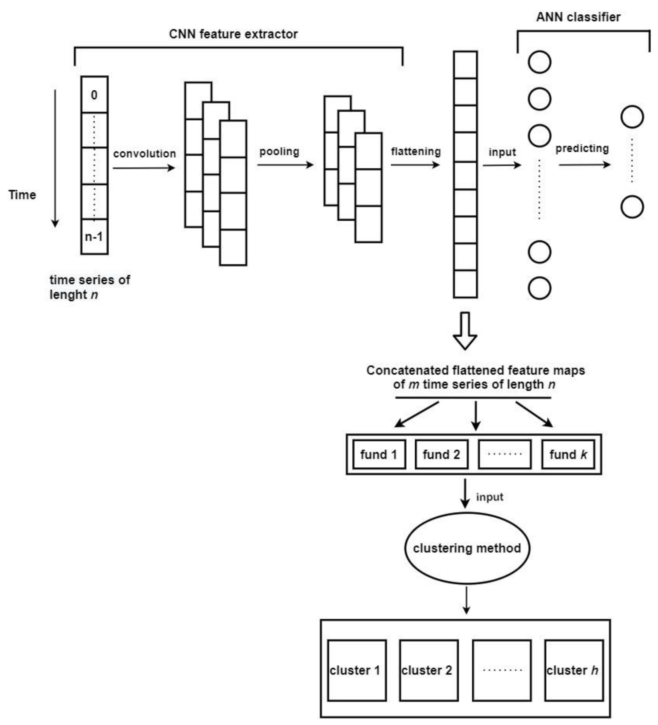
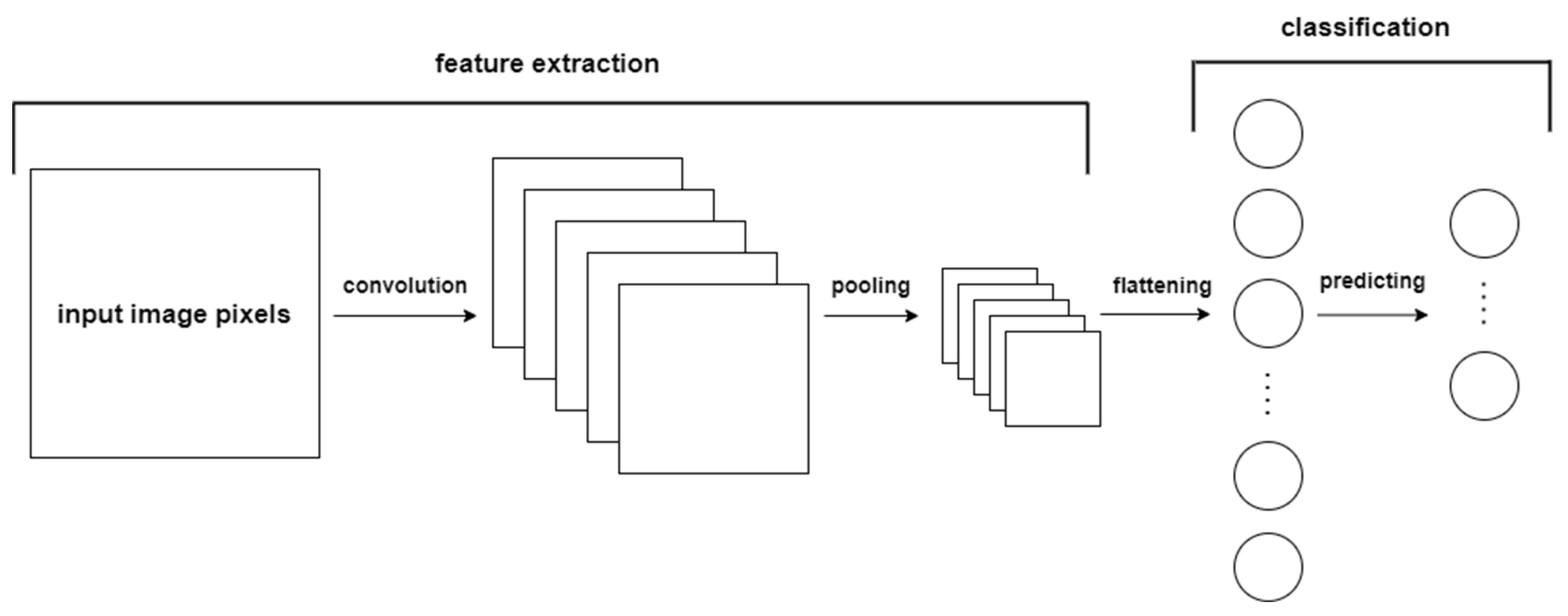
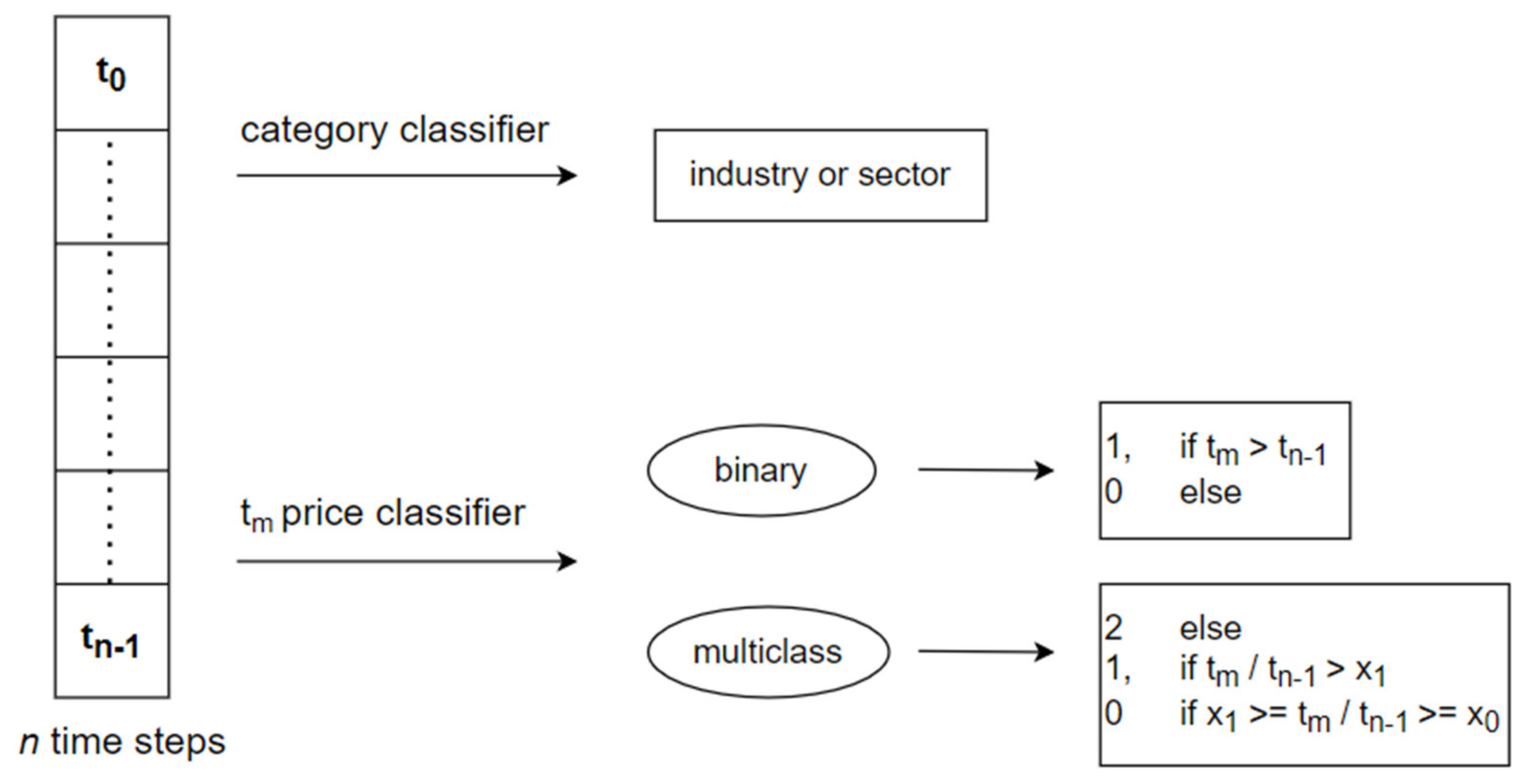
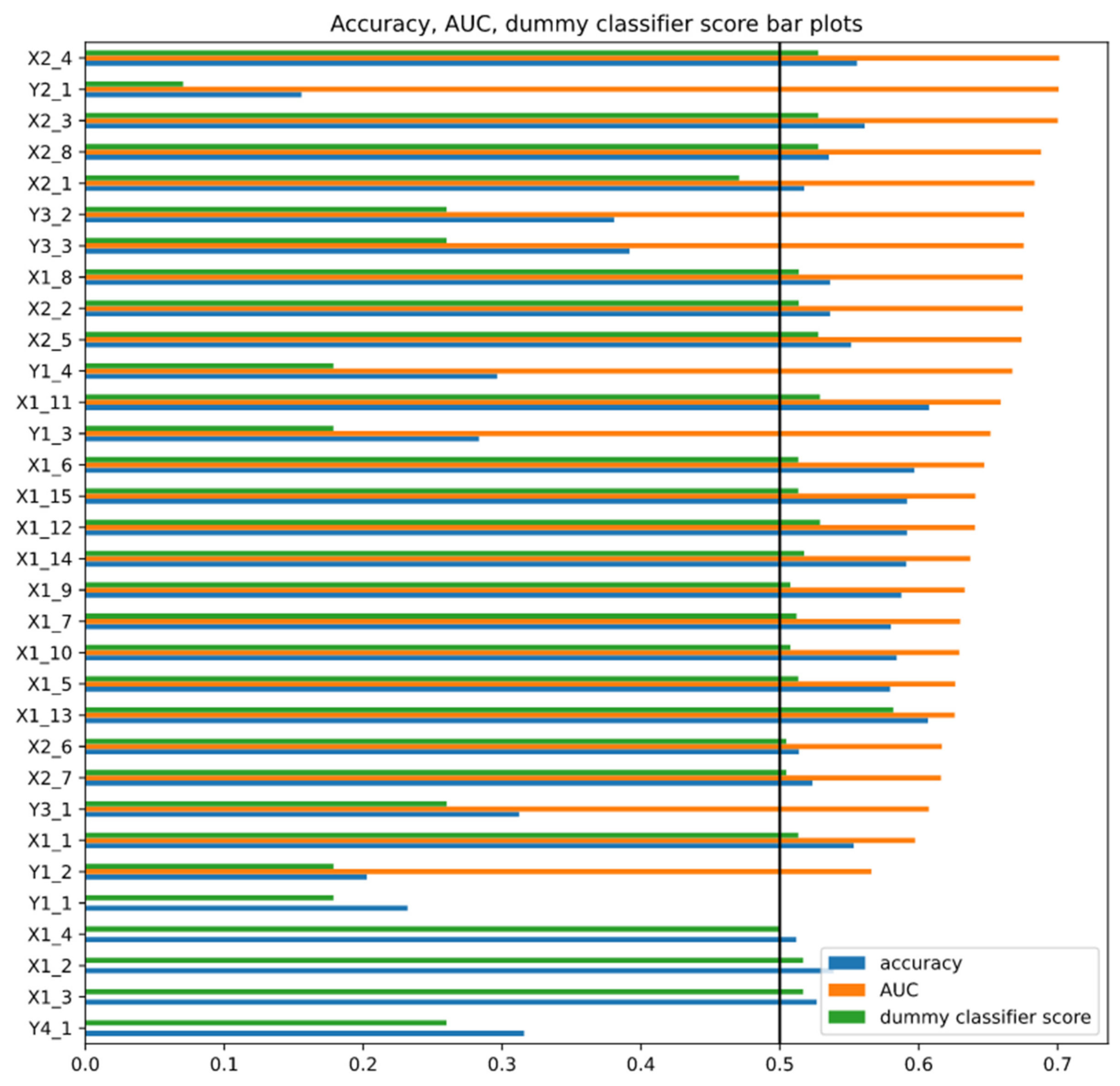
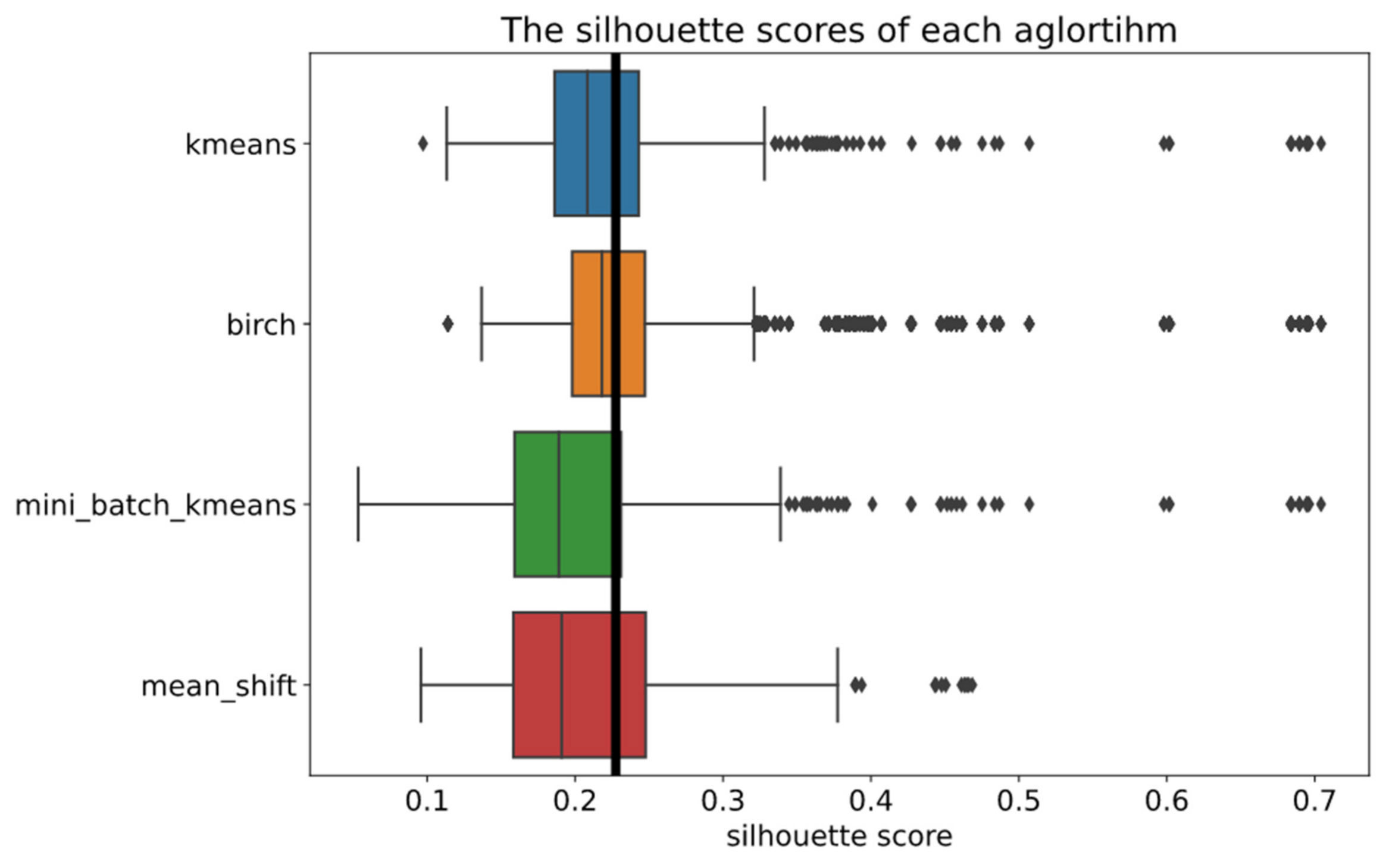
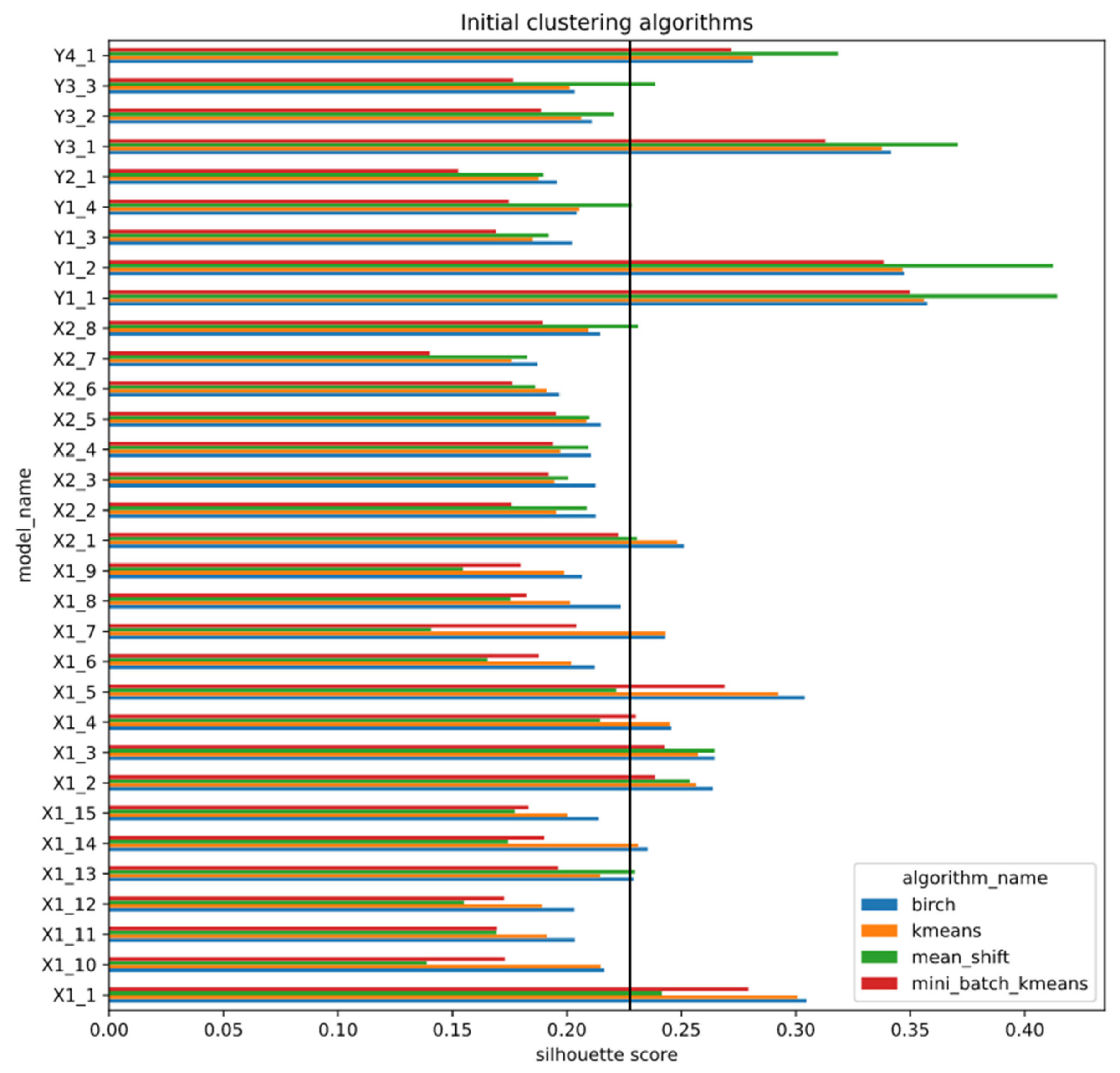
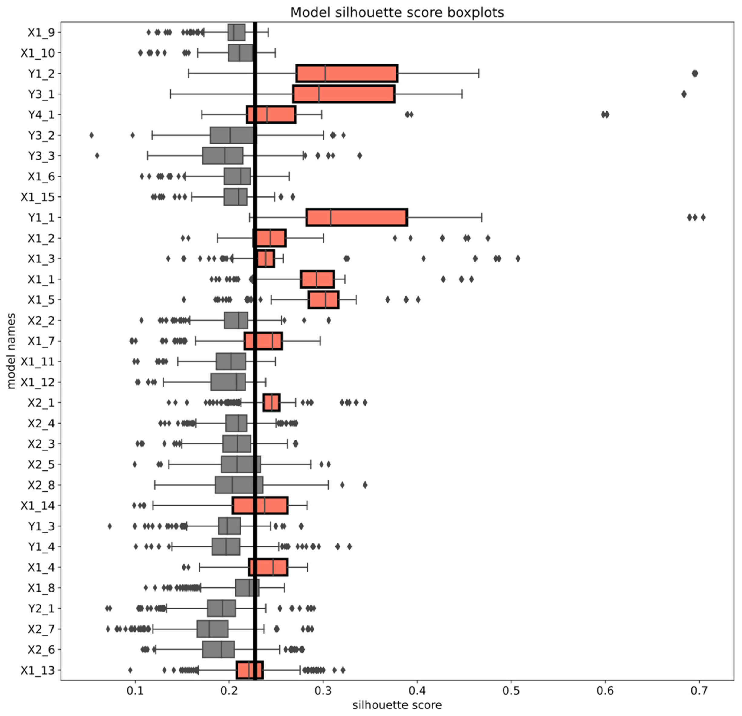
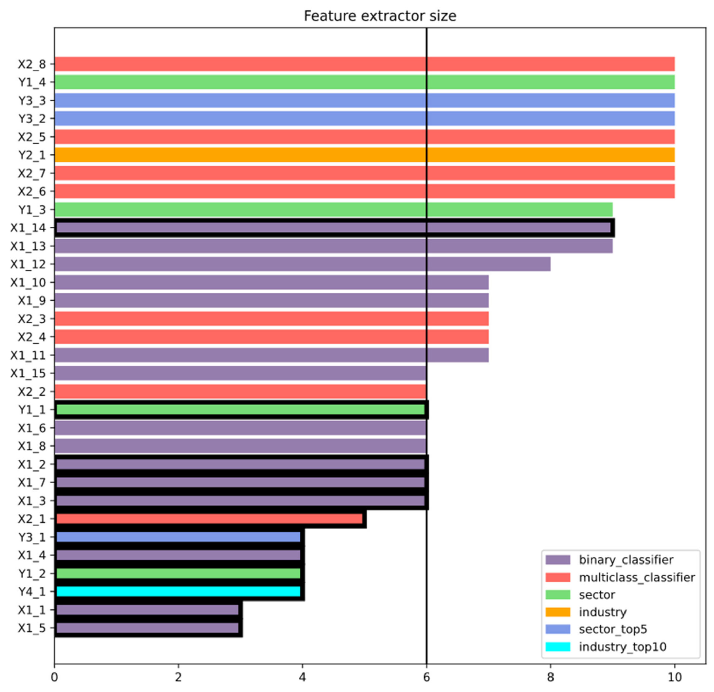
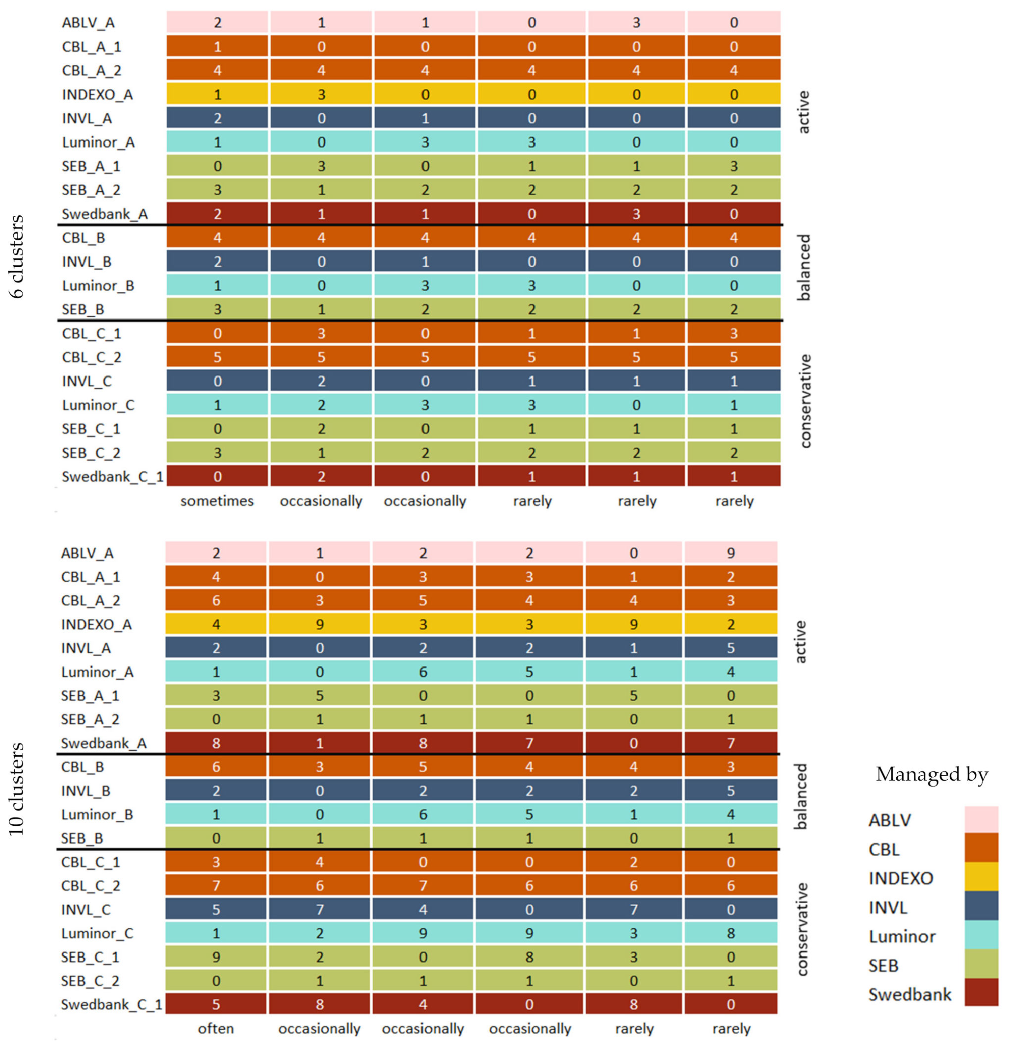
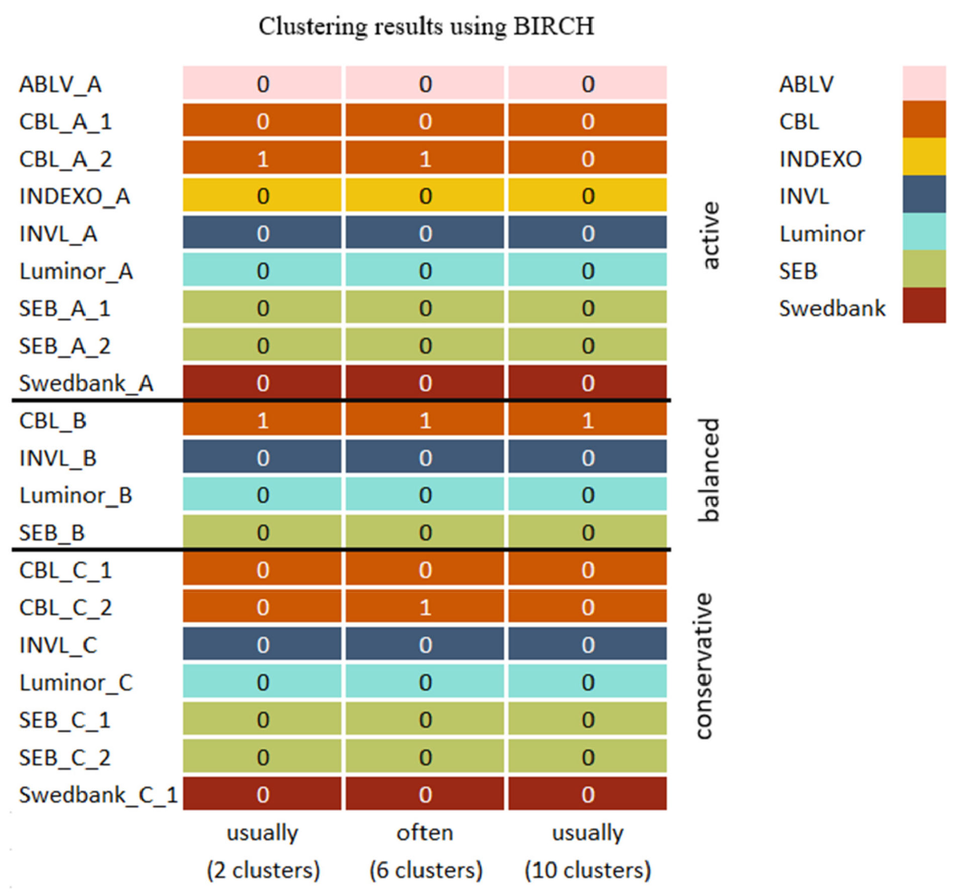
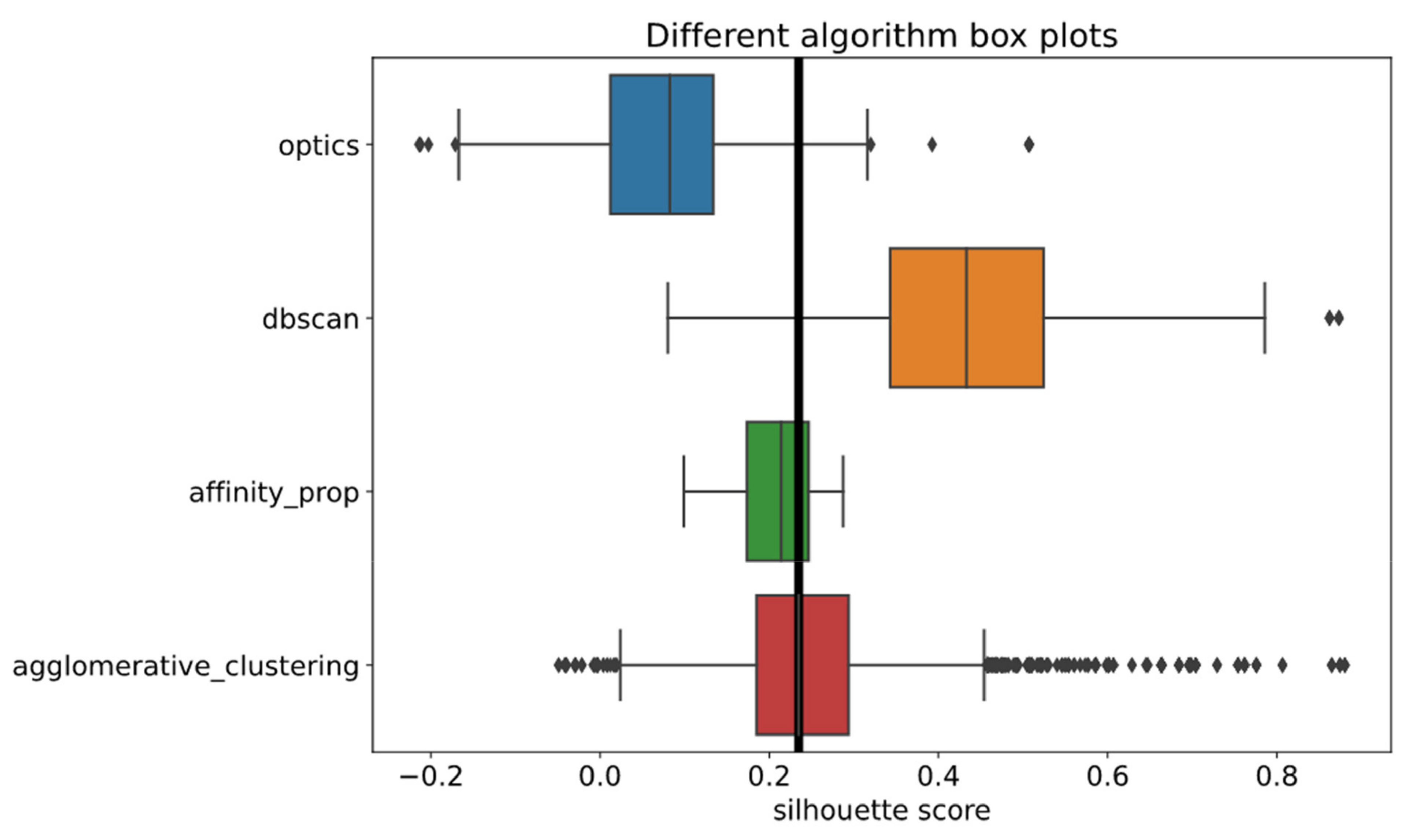
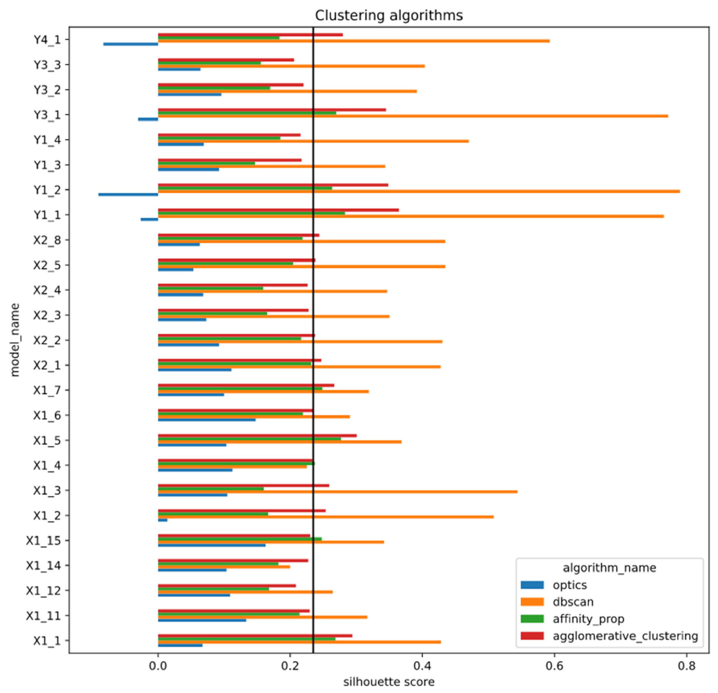
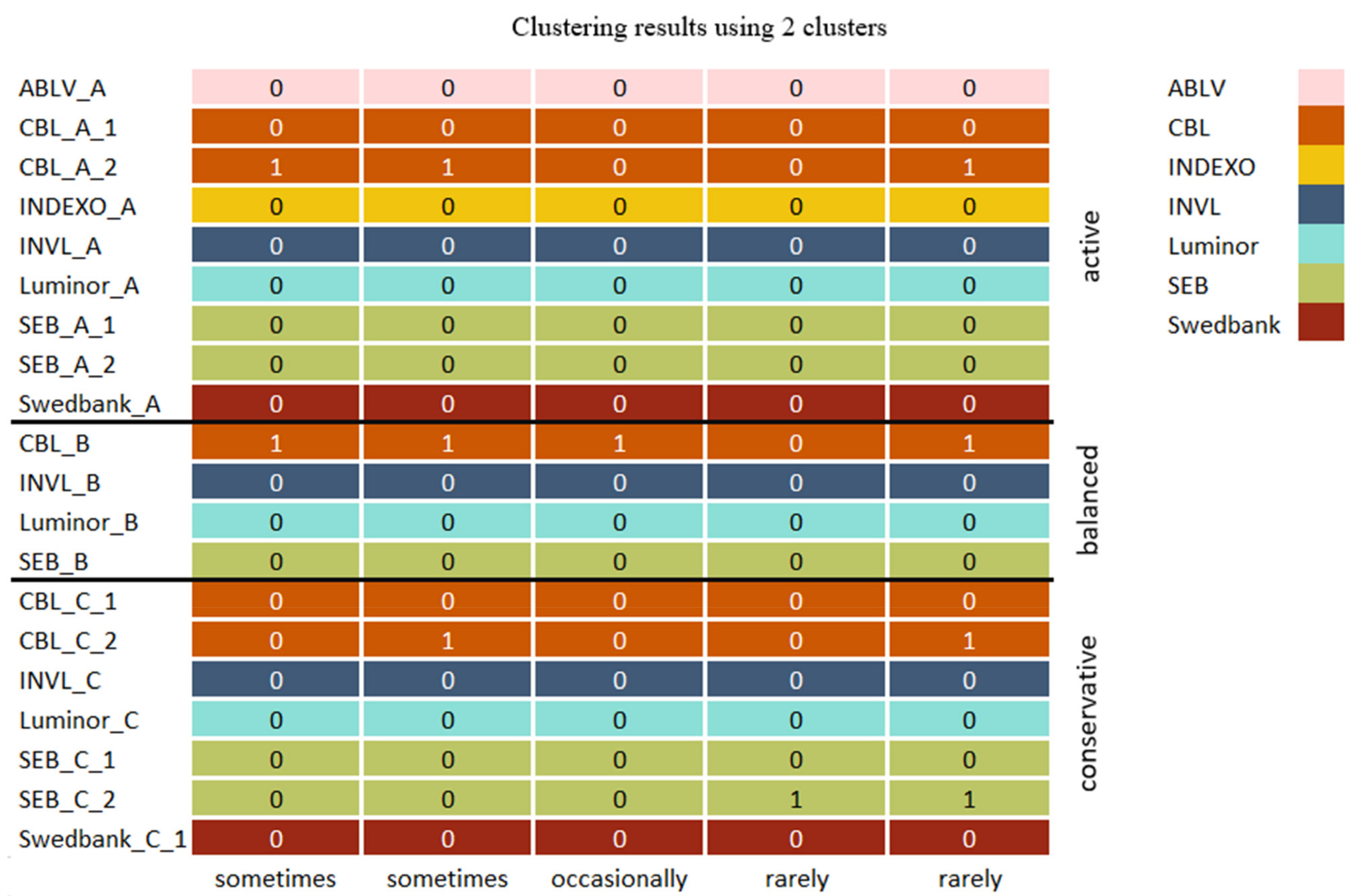
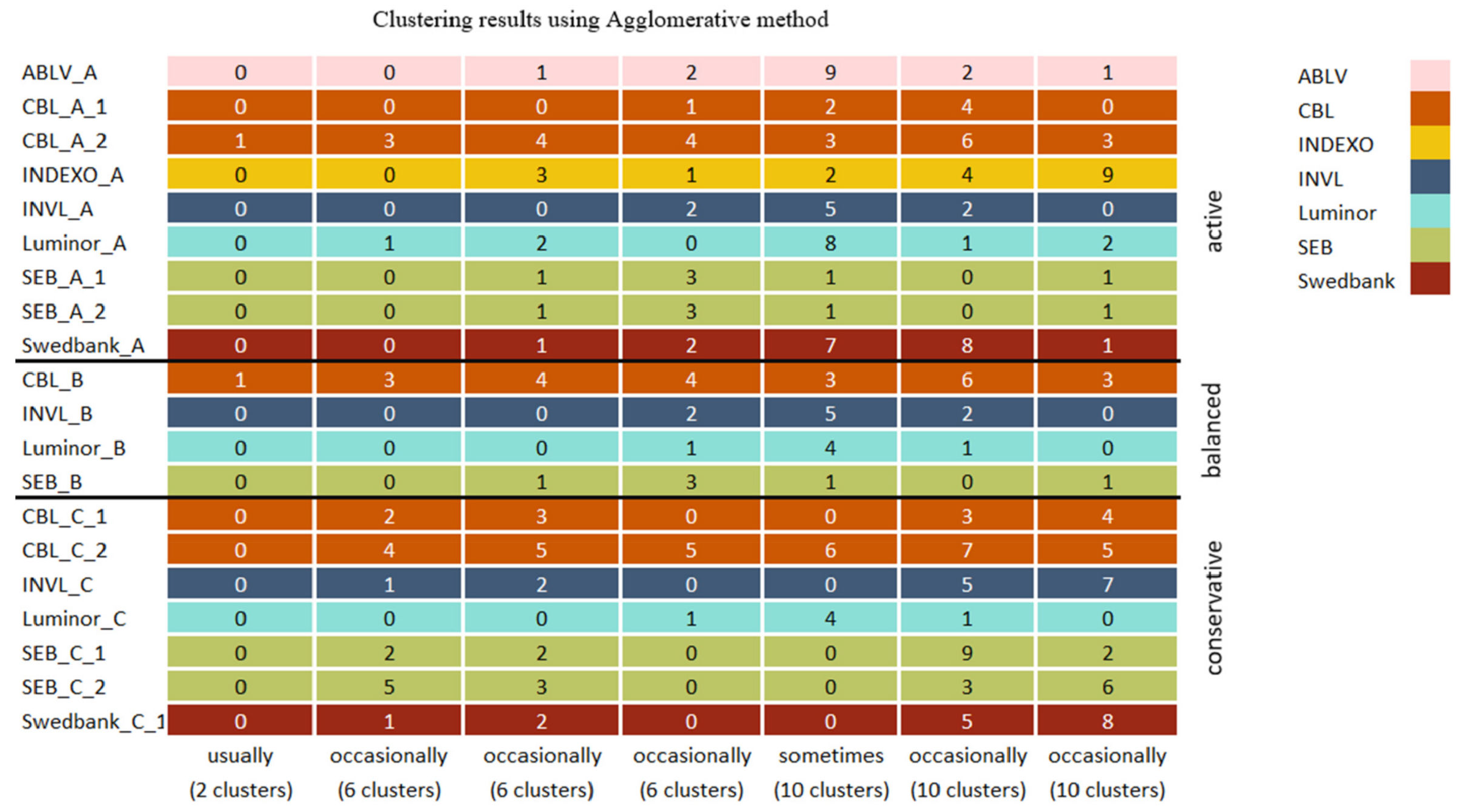
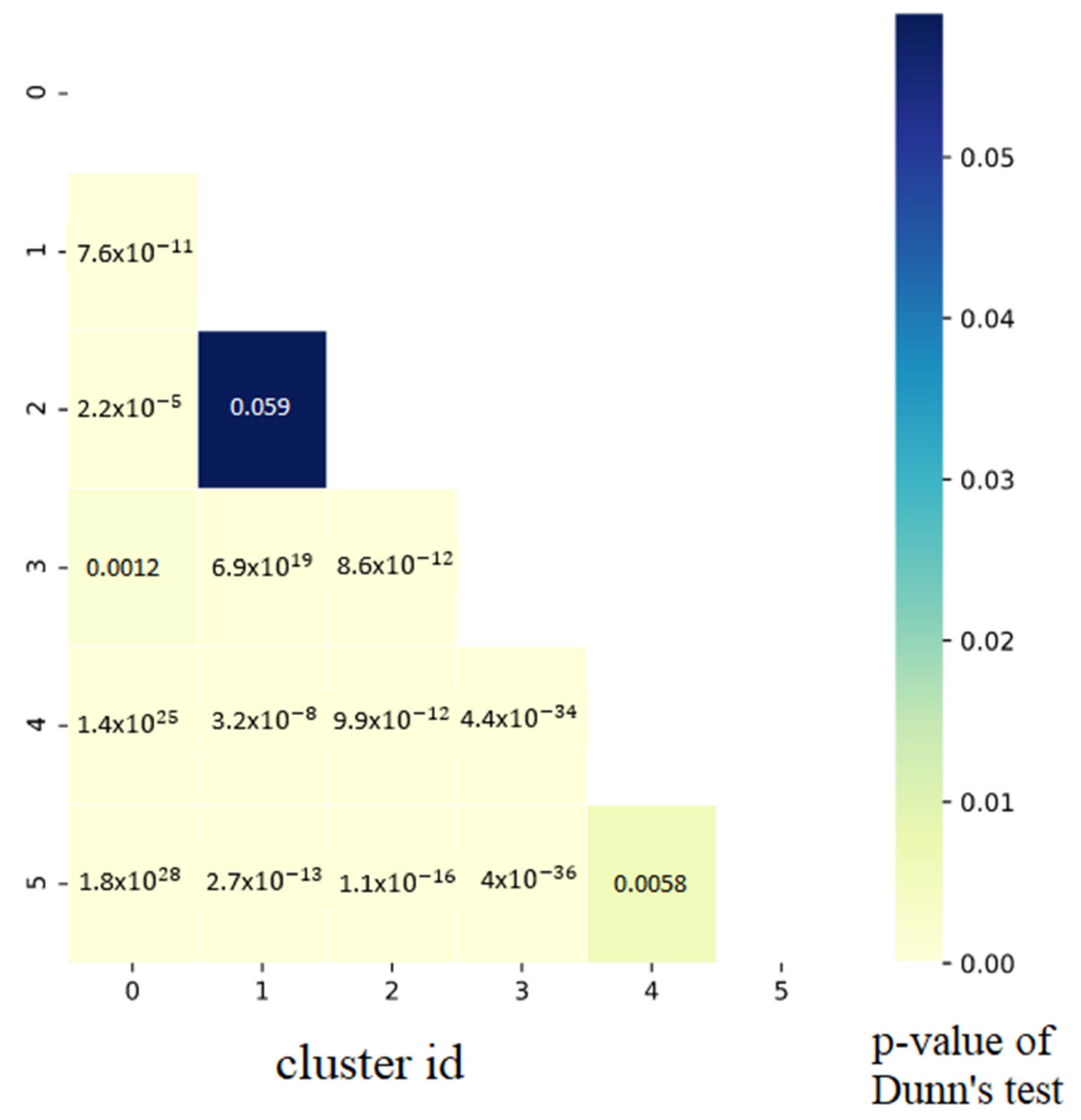
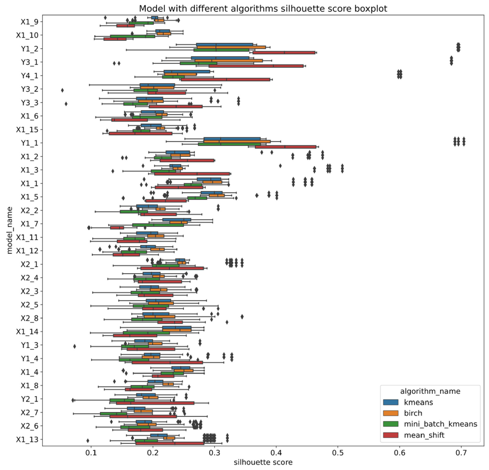
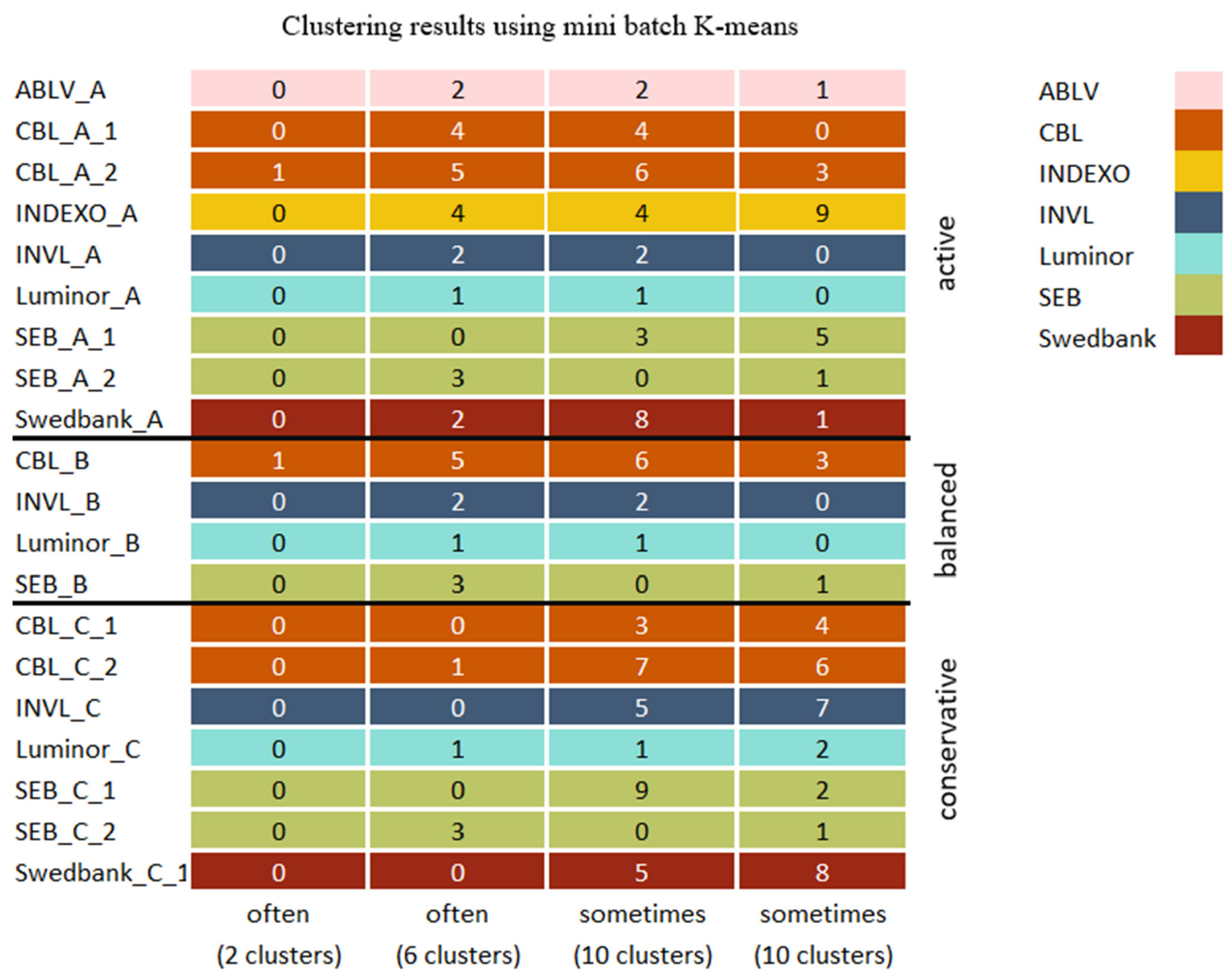
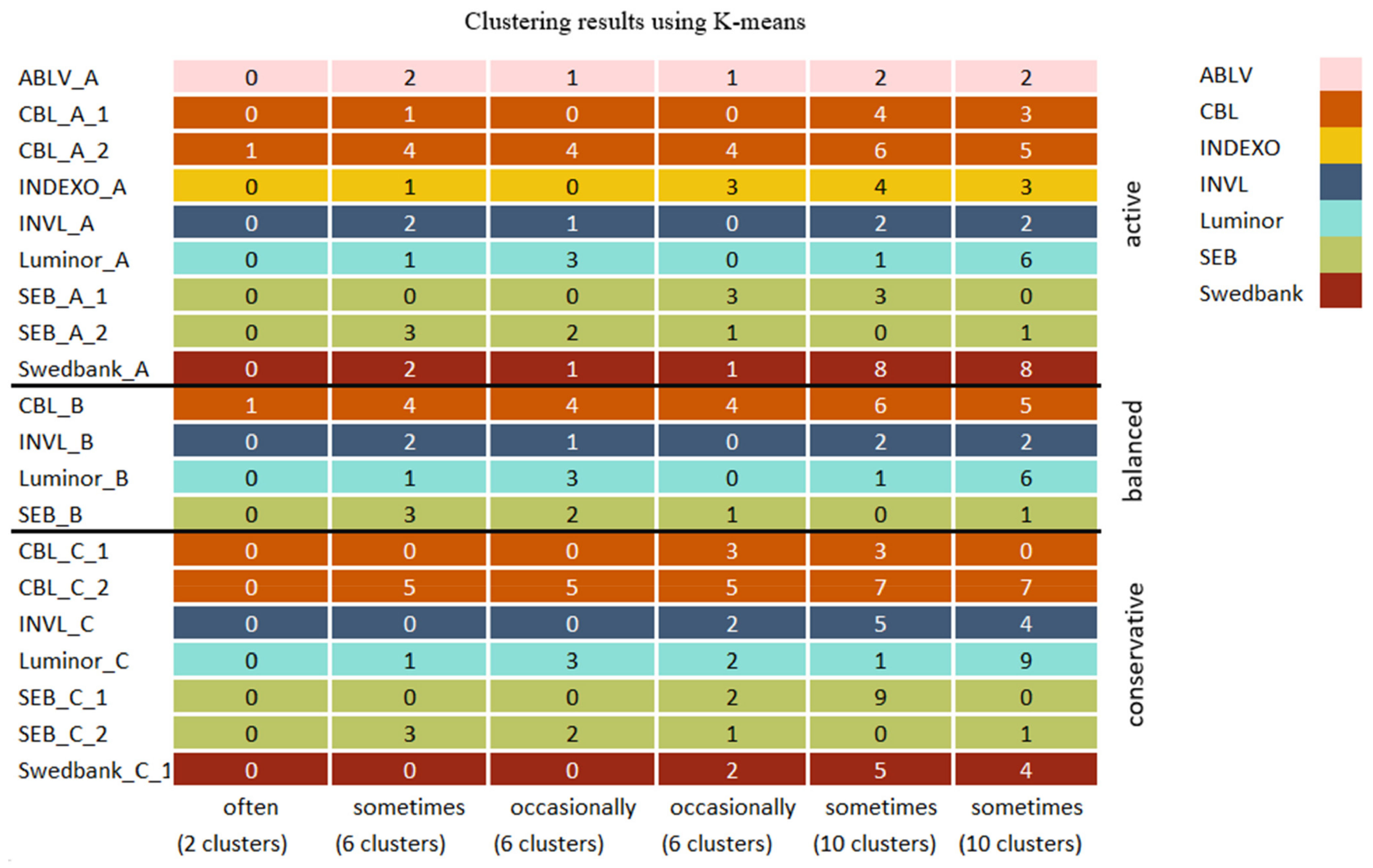
Table A1.
Trained model architectures. All convolutional layers use stride 1 and valid padding, max pooling uses a stride of 2 unless specified otherwise. Dropout uses a 0.2 parameter. The flatten layer is not specified unless dropout was not used. The values written near the dropout indicate the flattened output of the feature extractor. Some models have the same architecture but different input sizes. Therefore, the feature extractor output is different for such networks. Multiclass classifiers compare future prices with the price of the last input element value and predict to which category price change in percentages will fall. The mapping converts the price change percentage to one of the three categories. If the mapping uses a range of 3, then the price change label is determined by the range in which the value falls: 3% + increase, from −3% to 3%, or a greater decrease than −3%.
| Model Name and Classifier Type | Feature Extractor | Neural Network and Neurons |
|---|---|---|
| X1_6 (binary price classifier) | 16 kernels with size 2 | Dropout 896 |
| 32 kernels with size 3 | Dense 64 | |
| Max pooling | Dense 1 | |
| 64 kernels with size 5 | ||
| 128 kernels with size 5 | ||
| Max pooling | ||
| X1_15 (binary price classifier) | 16 kernels with size 2 | Dropout 896 |
| 32 kernels with size 3 | Dense 64 | |
| Max pooling | Dense 1 | |
| 64 kernels with size 5 | ||
| 128 kernels with size 5 | ||
| Max pooling | ||
| X2_1 (multiclass price classifier) | 32 kernels with size 2 | Dropout 1736 |
| 64 kernels with size 3 | Dense 256 | |
| Max pooling | Dropout | |
| 124 kernels with size 5 | Dense 64 | |
| Max pooling | Dense 3 | |
| X2_4 (multiclass price classifier) X2_3 (multiclass price classifier) | 32 kernels with size 2 | Dropout 3072 |
| 64 kernels with size 3 | Dense 64 | |
| 64 kernels with size 3 | Dense 3 | |
| Max pooling | ||
| 128 kernels with size 5 | ||
| 256 kernels with size 3 | ||
| Max pooling | ||
| Y1_1 (sector classifier) | 16 kernels with size 2 | Flatten 320 |
| Max pooling | Dense 64 | |
| 32 kernels with size 2 | Dense 12 | |
| Max pooling | ||
| 64 kernels with size 2 | ||
| Max pooling | ||
| Y1_2 (sector classifier) | 32 kernels with size 2 | Dropout 256 |
| Max pooling stride 3 | Dense 64 | |
| 64 kernels with size 2 | Dense 12 | |
| Max pooling stride 3 | ||
| X1_4 (binary price classifier) | 32 kernels with size 2 | Dropout 512 |
| Max pooling stride 2 | Dense 32 | |
| 32 kernels with size 2 | Dense 1 | |
| Max pooling stride 2 | ||
| Y2_1 (industry classifier) | 32 kernels with size 2 | Dropout 2304 |
| 64 kernels with size 3 | Dense 64 | |
| 64 kernels with size 2 | Dense 128 | |
| Max pooling | ||
| 128 kernels with size 2 | ||
| 256 kernels with size 3 | ||
| Max pooling | ||
| 256 kernels with size 3 | ||
| 256 kernels with size 3 | ||
| Max pooling | ||
| X2_2 (multiclass price classifier) | 64 kernels with size 2 | Dropout 2304 |
| 128 kernels with size 3 | Dense 256 | |
| Max pooling | Dense 64 | |
| 128 kernels with size 5 | Dense 3 | |
| 256 kernels with size 2 | ||
| Max pooling | ||
| X2_7 (multiclass price classifier) X2_6 (multiclass price classifier) | 32 kernels with size 2 | Dropout 2560 |
| 64 kernels with size 2 | Dense 256 | |
| 64 kernels with size 3 | Dense 64 | |
| Max pooling | Dense 3 (used range 5) | |
| 128 kernels with size 2 | ||
| 256 kernels with size 3 | ||
| Max pooling | ||
| 256 kernels with size 2 | ||
| 256 kernels with size 2 | ||
| Max pooling | ||
| X1_14 (binary price classifier) X1_13 (binary price classifier) | 32 kernels with size 2 | Dropout 1265, 2530 |
| 64 kernels with size 3 | Dense 256 | |
| 64 kernels with size 5 | Dense 64 | |
| Max pooling | Dense 1 | |
| 128 kernels with size 2 | ||
| 256 kernels with size 3 | ||
| Max pooling | ||
| 253 kernels with size 3 | ||
| Max pooling | ||
| X1_8 (binary price classifier) X1_7 (binary price classifier) | 64 kernels with size 2 | Dropout 4096, 2304 |
| 128 kernels with size 3 | Dense 256 | |
| Max pooling | Dense 64 | |
| 128 kernels with size 5 | Dense 1 | |
| 256 kernels with size 2 | ||
| Max pooling | ||
| X1_9 (binary price classifier) X1_10 (binary price classifier) X1_11 (binary price classifier) | 32 kernels with size 2 | Dropout 1280, 2560 |
| 64 kernels with size 3 | Dense 64 | |
| 64 kernels with size 3 | Dense 1 | |
| Max pooling | ||
| 128 kernels with size 5 | ||
| 256 kernels with size 3 | ||
| Max pooling | ||
| X1_12 (binary price classifier) | 64 kernels with size 2 | Dropout 1024 |
| 64 kernels with size 3 | Dense 256 | |
| Max pooling | Dense 64 | |
| 128 kernels with size 2 | Dense 1 | |
| Max pooling | ||
| 128 kernels with size 6 | ||
| 256 kernels with size 3 | ||
| Max pooling | ||
| Y3_1 (sector classifier taking top 5 most frequent sectors) | 32 kernels with size 2 | Dropout 288 |
| Max pooling | Dense 32 | |
| 32 kernels with size 2 | Dense 5 | |
| Max pooling | ||
| Y3_2 (sector classifier taking top 5 most frequent sectors) Y3_3 (sector classifier taking top 5 most frequent sectors) | 32 kernels with size 2 | Dropout 512 |
| 64 kernels with size 3 | Dense 64 | |
| 64 kernels with size 2 | Dense 5 | |
| Max pooling | ||
| 128 kernels with size 2 | ||
| 256 kernels with size 3 | ||
| Max pooling | ||
| 256 kernels with size 3 | ||
| 256 kernels with size 3 | ||
| Max pooling | ||
| Y1_3 (sector classifier) | 32 kernels with size 2 | Dropout 1265 |
| 64 kernels with size 3 | Dense 64 | |
| 64 kernels with size 2 | Dense 12 | |
| Max pooling | ||
| 128 kernels with size 2 | ||
| 256 kernels with size 3 | ||
| Max pooling | ||
| 253 kernels with size 2 | ||
| Y1_4 (sector classifier) X1_2 (binary price classifier) | 32 kernels with size 2 | Dropout 1024, 1408 |
| 64 kernels with size 3 | Dense 64 | |
| 64 kernels with size 2 | Dense 12, 1 | |
| Max pooling | ||
| 128 kernels with size 2 | ||
| 256 kernels with size 3 | ||
| Max pooling | ||
| 256 kernels with size 3 | ||
| 256 kernels with size 3 | ||
| X1_3 (binary price classifier) | 16 kernels with size 2 | Dropout 1408 |
| 32 kernels with size 2 | Dense 64 | |
| Max pooling | Dense 1 | |
| 64 kernels with size 2 | ||
| 128 kernels with size 2 | ||
| Max pooling | ||
| X1_1 (binary price classifier) X1_5 (binary price classifier) | 64 kernels with size 2 | Dropout 256 |
| 128 kernels with size 3 | Dense 64 | |
| Max pooling | Dense 1 | |
| Y4_1 (industry classifier taking top 100 most frequent industries) | 32 kernels with size 2 | Dropout 288 |
| Max pooling | Dense 32 | |
| 32 kernels with size 2 | Dense 10 | |
| Max pooling | ||
| X2_5 (multiclass price classifier) | 32 kernels with size 2 | Dropout 768 |
| 64 kernels with size 3 | Dense 64 | |
| 64 kernels with size 2 | Dense 3 | |
| Max pooling | ||
| 128 kernels with size 5 | ||
| 128 kernels with size 3 | ||
| Max pooling | ||
| 256 kernels with size 3 | ||
| 256 kernels with size 5 | ||
| Max pooling | ||
| X2_8 (multiclass price classifier) | 32 kernels with size 2 | Dropout 256 |
| 64 kernels with size 3 | Dense 64 | |
| 64 kernels with size 3 | Dense 3 | |
| Max pooling | ||
| 128 kernels with size 4 | ||
| 128 kernels with size 5 | ||
| Max pooling | ||
| 256 kernels with size 3 | ||
| 256 kernels with size 3 | ||
| Max pooling |
Table A2.
The model output and input sizes predict price time-steps, overlap, epochs trained, accuracy, AUC, and dummy scores. Only price classifiers have defined predict price time-steps. Overlap indicates whether the training and validation dataset time-series could overlap within observations during the data preparation stage.
| Model Name | Input Size | Predict Price Timestep | Overlap | Epochs | Accuracy | AUC | Dummy Score |
|---|---|---|---|---|---|---|---|
| X1_15 | 50 | 5 | 5 | 300 | 0.5916 | 0.6408 | 0.5133 |
| X1_6 | 50 | 5 | 5 | 400 | 0.5969 | 0.6472 | 0.5133 |
| X1_5 | 50 | 5 | 0 | 400 | 0.5794 | 0.6263 | 0.5133 |
| X2_1 | 60 | 5 | 0 | 300 | 0.5176 | 0.6834 | 0.4707 |
| X2_5 | 60 | 5 | 0 | 200 | 0.5514 | 0.6741 | 0.5277 |
| X2_8 | 60 | 5 | 0 | 200 | 0.5353 | 0.6881 | 0.5277 |
| X2_3 | 60 | 5 | 5 | 200 | 0.5611 | 0.7002 | 0.5277 |
| X2_4 | 60 | 5 | 10 | 200 | 0.5556 | 0.7012 | 0.5277 |
| X1_9 | 30 | 5 | 5 | 100 | 0.5875 | 0.6331 | 0.5076 |
| X1_10 | 30 | 5 | 5 | 100 | 0.5841 | 0.6292 | 0.5076 |
| X1_11 | 50 | 5 | 5 | 200 | 0.6074 | 0.6590 | 0.5289 |
| X1_14 | 60 | 10 | 10 | 100 | 0.5910 | 0.6371 | 0.5175 |
| X1_13 | 100 | 80 | 30 | 100 | 0.6067 | 0.6259 | 0.5817 |
| X2_7 | 100 | 80 | 30 | 200 | 0.5235 | 0.6160 | 0.5047 |
| X2_6 | 100 | 80 | 30 | 100 | 0.5137 | 0.6167 | 0.5047 |
| Y1_3 | 60 | - | 0 | 200 | 0.2834 | 0.6516 | 0.1786 |
| Y1_4 | 60 | - | 0 | 200 | 0.2965 | 0.6674 | 0.1786 |
| Y3_2 | 40 | - | 0 | 200 | 0.3807 | 0.6759 | 0.2601 |
| Y3_3 | 40 | - | 0 | 205 | 0.3918 | 0.6756 | 0.2601 |
| Y2_1 | 100 | - | 0 | 400 | 0.1556 | 0.7007 | 0.0704 |
| X1_12 | 50 | 5 | 5 | 200 | 0.5915 | 0.6405 | 0.5289 |
| X2_2 | 50 | 15 | 20 | 200 | 0.5361 | 0.6749 | 0.5136 |
| X1_8 | 80 | 15 | 20 | 200 | 0.5800 | 0.6298 | 0.512 |
| Y1_1 | 50 | - | 0 | 200 | 0.2320 | - | 0.1786 |
| X1_4 | 70 | 7 | 0 | 200 | 0.5118 | - | 0.5 |
| Y1_2 | 40 | - | 0 | 150 | 0.2026 | 0.5659 | 0.1786 |
| X1_7 | 50 | 15 | 20 | 200 | 0.5800 | 0.6298 | 0.5120 |
| Y3_1 | 40 | - | 0 | 180 | 0.3123 | 0.6072 | 0.2601 |
| X1_2 | 50 | 5 | 0 | 200 | 0.5388 | - | 0.5168 |
| X1_3 | 50 | 10 | 0 | 200 | 0.5265 | - | 0.5168 |
| X1_1 | 50 | 5 | 0 | 400 | 0.5532 | 0.5974 | 0.5133 |
| Y4_1 | 40 | - | 0 | 200 | 0.3159 | - | 0.26 |
Table A3.
Clustering algorithm parameters.
| Algorithm Name | Parameter Name | Parameter Value | |
|---|---|---|---|
| K-means, mini batch K-means | n_clusters | 2 to 10 | |
| Birch | n_clusters | 2 to 10 | |
| threshold | 0.1 to 1 with 0.1 step | ||
| Mean shift | bin_seeding | true, false | |
| cluster_all | true, false | ||
| Affinity propagation | damping | 0.5 to 1 with 0.05 step | |
| DBSCAN | eps | 0.3, 0.5 or 0.8 | |
| Optics | leaf_size | 30 | |
| DBSCAN, Optics | min_samples | 3, 5 or 10 | |
| algorithm, metric | kd_tree | Euclidean, l2, Minkowski, Manhattan, Chebyshev | |
| ball_tree | Euclidean, L2, Minkowski, Manhattan, L1, Chebyshev, Wminkowski, Canberra, Bray–Curtis | ||
| brute | Euclidean, L2, Minkowski, Manhattan, Chebyshev, Wminkowski, Canberra, Braycurtis, Correlation, Cosine, Squeclidean | ||
| Agglomerative | n_clusters | 2 to 10 | |
| linkage | Ward, Average, Complete, or single | ||
| affinity | Euclidean, L1, L2, Manhattan, Cosine | ||
Appendix B. Clustering Results
Figure A1.
Silhouette score box plots for each model using different algorithms.

Figure A2.
Top 50 best mini batch K-means algorithm results based on silhouette score using different number of clusters. The cluster value is noted in the parentheses, and the most often occurring combinations are visualized.
Figure A2.
Top 50 best mini batch K-means algorithm results based on silhouette score using different number of clusters. The cluster value is noted in the parentheses, and the most often occurring combinations are visualized.

Figure A3.
Top 50 best K-means algorithm results based on silhouette score using a different number of clusters. The cluster value is noted in the parentheses, and most often occurring combinations are visualized.
Figure A3.
Top 50 best K-means algorithm results based on silhouette score using a different number of clusters. The cluster value is noted in the parentheses, and most often occurring combinations are visualized.

Table A4.
Top 100 best affinity propagation algorithm results based on silhouette score using different parameters that result in a different number of clusters. The table shows the composition of often occurring cluster combinations when six clusters were used.
Table A4.
Top 100 best affinity propagation algorithm results based on silhouette score using different parameters that result in a different number of clusters. The table shows the composition of often occurring cluster combinations when six clusters were used.
| Cluster 0 | Cluster 1 | Cluster 2 | Cluster 3 | Cluster 4 | Cluster 5 |
|---|---|---|---|---|---|
| CBL_C_1 INVL_C SEB_C_1 SEB_C_2 Swedbank_C_1 | CBL_A_1 INDEXO_A Luminor_A Luminor_B Luminor_C | ABLV_A INVL_A INVL_B Swedbank_A | SEB_A_1 SEB_A_2 SEB_B | CBL_A_2 CBL_B | CBL_C_2 |
Appendix C. Best Parameters and Models for Each Clustering Algorithm
Table A5.
Best parameters of each algorithm with the number of clusters used equally to 2, 6, or 10. The algorithm parameters column is empty when the best results depend on the model. The best model column is empty if the best result achieved depended mainly on the method parameters.
Table A5.
Best parameters of each algorithm with the number of clusters used equally to 2, 6, or 10. The algorithm parameters column is empty when the best results depend on the model. The best model column is empty if the best result achieved depended mainly on the method parameters.
| Algorithm Name | Clusters | Total Combinations | Mean Silhouette Score | Top Taken | Mean Silhouette Score Top | Best Model | Algorithm Parameters |
|---|---|---|---|---|---|---|---|
| K-means | 2 | 152 | 0.2638 | 10 | 0.6916 | Y1_1, Y1_2, Y3_1 | - |
| K-means | 6 | 152 | 0.2184 | 10 | 0.31 | Y1_1 | - |
| K-means | 10 | 152 | 0.2064 | 10 | 0.2931 | X1_5, X1_1, Y1_1 | - |
| BIRCH | 2 | 1368 | 0.2746 | 10 | 0.7035 | Y1_1 | - |
| BIRCH | 6 | 1368 | 0.228 | 10 | 0.3266 | X1_5 | - |
| BIRCH | 10 | 1368 | 0.2165 | 10 | 0.314 | X1_5 | - |
| Mini batch K-means | 2 | 152 | 0.2556 | 10 | 0.6916 | Y1_1, Y1_2, Y3_1 | - |
| Mini batch K-means | 6 | 152 | 0.2017 | 10 | 0.303 | Y1_1, Y1_2, Y3_1 | - |
| Mini batch K-means | 10 | 152 | 0.1777 | 10 | 0.2788 | X1_5 | - |
| Mean shift | 2 | 117 | 0.1856 | 10 | 0.2859 | Y2_1, X2_7 | - |
| Agglomerative clustering | 2 | 400 | 0.421 | 10 | 0.8666 | Y1_1, Y1_2, Y3_1 | Affinity: cosine |
| Agglomerative clustering | 6 | 400 | 0.2216 | 10 | 0.4354 | - | Linkage: average or complete; Affinity: cosine |
| Agglomerative clustering | 10 | 400 | 0.2125 | 10 | 0.4293 | - | Linkage: average or complete; Affinity: cosine |
| OPTICS | 2 | 382 | 0.0813 | 10 | 0.3825 | X1_3 | - |
| OPTICS | 10 | 1 | 0.1928 | 1 | 0.1928 | X1_14 | Algorithm: ball_tree; Metric: Bray–Curtis |
| DBSCAN | 2 | 321 | 0.4583 | 10 | 0.8349 | Y1_1, Y1_2, Y3_1 | Algorithm: brute; Metric: correlation, Bray-Curtis |
| Affinity propagation | 6 | 99 | 0.2052 | 10 | 0.286 | Y1_1, X1_5 | Damping: 0.5, 0.55, 0.6 |
References
- Ganguli, S.; Dunnmon, J. Machine Learning for Better Models for Predicting Bond Prices. 2017. Available online: https://arxiv.org/abs/1705.01142 (accessed on 11 May 2021).
- OECD. Pension Market in Focus. 2019. Available online: https://www.oecd.org/daf/fin/private-pensions/Pension-Markets-in-Focus-2019.pdf (accessed on 11 May 2021).
- Kotecha, M.; Arthur, S.; Coutinho, S. Understanding the Relationship Between Pensioner Poverty and Material Deprivation, London. 2013; ISBN 9781909532144. Available online:https://assets.publishing.service.gov.uk/government/uploads/system/uploads/attachment_data/file/197675/rrep827.pdf (accessed on 11 May 2021).
- Lannoo, K.; Barslund, M.; Chmelar, A.; Werder, M.; Pension Schemes. Brussels, 2014: European Parliament’s Committee on Employment and Social Affairs. Available online: https://www.europarl.europa.eu/RegData/etudes/STUD/2014/536281/IPOL_STU(2014)536281_EN.pdf (accessed on 11 May 2021).
- Keohane, N.; Rowell, S.; Good Pensions. Introducing Social Pension Funds to the UK, London: Social Market Foundation. 2015. Available online: http://www.smf.co.uk/wp-content/uploads/2015/09/Social-Market-FoundationSMF-BSC-030915-Good-Pensions-Introducing-social-pension-funds-to-the-UK-FINAL.pdf (accessed on 11 May 2021).
- Pensions Europe. Pension Fund Statistics and Trends 2018. Available online: https://www.pensionseurope.eu (accessed on 11 May 2021).
- Bruder, B.; Culerier, L.; Roncalli, T. How to design target-date funds? SSRN Electron. J. 2013. [Google Scholar] [CrossRef] [Green Version]
- Donaldson, S.J.; Kinniry, F.M.; Mačiulis, V.; Patterson, A.J.; Dijoseph, M. Vanguard’s approach to target-date funds [interactive]. Available online: https://www.vanguard.com/ (accessed on 11 May 2021).
- Laursen, C.; Gkatzimas, I.; Jovanovic, B. TARGET DATE FUNDS Economic, Regulatory, and Legal Trends. 2017. Available online: https://brattlefiles.blob.core.windows.net/files/7164_target_date_funds_economic__regulatory__and_legal_trends.pdf (accessed on 11 May 2021).
- Tonks, I. Pension Fund Management and Investment Performance; Gordon, L.C., Munnell, A.H., Orszag, J.M., Eds.; The Oxford Handbook of Pensions and Retirement Income: Oxford, UK, 2006. [Google Scholar]
- Keeley, B.; Love, P. OECD Insights from Crisis to Recovery the Causes, Course and Consequences of the Great Recession: The Causes, Course and Consequences of the Great Recession; OECD Publishing: Paris, France, 2010. [Google Scholar] [CrossRef]
- Manapensija: Current Statistics. Available online: https://www.manapensija.lv/en/2nd-pension-pillar/statistics/ (accessed on 30 April 2021).
- Kabašinskas, A.; Maggioni, F.; Šutienė, K.; Valakevičius, E. A Multistage Risk-Averse Stochastic Programming Model for Personal Savings Accrual: The Evidence from Lithuania—Annals of Operations Research; Springer: New York, NY, USA, 2018; pp. 1–28. ISSN 0254-5330. [Google Scholar] [CrossRef]
- Financial and Capital Market Commission. Available online: https://www.fktk.lv/ (accessed on 10 August 2021).
- Jefremova, J.; Mietule, I. Investment trends of Latvian pension funds after the 2008 financial crisis. In Proceedings of the 5th International Conference on Accounting, Auditing and Taxation, Tallinn, Estonia, 8–9 December 2016. [Google Scholar] [CrossRef] [Green Version]
- Rajevska, O.; Rajevska, F. Effectiveness of the Latvian pension system in addressing the problem of poverty among the elderly. In Proceedings of the Pensions Conference 2018, Lodz, Poland, 19–20 April 2018. [Google Scholar]
- Serge-Lopez, W.-T.; Wamba, S.F.; Kamdjoug, J.R.K.; Wanko, C.E.T.W. Influence of Artificial Intelligence (AI) on firm performance: The business value of AI-based transformation projects. Bus. Process. Manag. J. 2020, 26, 1893–1924. Available online: https://www.emerald.com/insight/content/doi/10.1108/BPMJ-10-2019-0411/full/html#loginreload (accessed on 11 May 2021).
- Chen, M.Y.; Chiang, H.S.; Lughofer, E. Deep learning: Emerging trends, applications and research challenges. Soft Comput. 2020, 24, 7835–7838. [Google Scholar] [CrossRef]
- Zhao, B.; Lu, H.; Chen, S.; Liu, J.; Wu, D. Convolutional neural networks for time series classification. J. Syst. Eng. Electron. 2017, 28, 162–169. [Google Scholar] [CrossRef]
- Umuhoza, E.; Ntirushwamaboko, D.; Awuah, J.; Birir, B. Using unsupervised machine learning techniques for behavioral-based credit card users segmentation in Africa. S. Afr. Inst. Electr. Eng. 2020, 111, 95–101. Available online: http://www.scielo.org.za/pdf/arj/v111n3/02.pdf (accessed on 11 May 2021). [CrossRef]
- Xu, D.; Tian, Y. A comprehensive survey of clustering algorithms. Ann. Data Sci. 2015, 2, 165–193. [Google Scholar] [CrossRef] [Green Version]
- Javedac, A.; Leeac, B.S.; Rizzobc, D.M. A benchmark study on time series clustering. Mach. Learn. Appl. 2020, 1, 1–13. [Google Scholar]
- Lei, Q.; Yi, J.; Vaculin, R.; Wu, L.; Dhillon, I.S. Similarity preserving representation learning for time series clustering. In Proceedings of the Twenty Eighth International Joint Conference on Artificial Intelligence, Macao, China, 10–16 August 2019; {IJCAI-19} 2019. Available online: https://www.ijcai.org/proceedings/2019/394 (accessed on 11 May 2021).
- Guerin, J.; Gibaru, O.; Thiery, S.; Nyiri, E. CNN features are also great at unsupervised classification [interactive]. arXiv 2017, arXiv:1707.01700. [Google Scholar]
- Chen, W.; Langrene, N. Deep Neural Network for Optimal Retirement Consumption in Defined Contribution Pension System 2020. Available online: https://arxiv.org/pdf/2007.09911.pdf (accessed on 10 May 2021).
- Sasaki, T.; Koizumi, H.; Tajiri, T.; Kitano, H. A Study on the Use of Artificial Intelligence within Government Pension Investment Fund’s Investment Management Practices (Summary Report), Tokyo, 2017: Government Pension Investment Fund. Available online: https://www.gpif.go.jp/en/investment/research_2017_1_en.pdf (accessed on 11 May 2021).
- Barna, F.; Seulean, V.; Mos, M.L. A cluster analysis of OECD pension funds. Timis. J. Econ. 2011, 4, 143–148. [Google Scholar]
- Kabašinskas, A.; Šutienė, K.; Kopa, M.; Valakevičius, E. The risk-return profile of Lithuanian private pension funds. Ecnonomic Res. 2017, 30, 1611–1630. [Google Scholar] [CrossRef] [Green Version]
- Kaggle: Daily Historical Stock Prices 1970–2018. Available online: https://www.kaggle.com/ehallmar/daily-historical-stock-prices-1970-2018 (accessed on 10 March 2021).
- Keras. Developer Guides. Available online: https://keras.io/guides/ (accessed on 11 May 2021).
- Wandb. Fundamentals of Neural Networks. 2019. Available online: https://wandb.ai/site/articles/fundamentals-of-neural-networks (accessed on 11 May 2021).
- Kingma, D.P.; Lei, B.; Adam, J. A Method for Stochastic Optimization. 2015. Available online: https://arxiv.org/abs/1412.6980 (accessed on 10 May 2021).
- Yoon, K. Convolutional Neural Networks for Sentence Classification. 2014. Available online: https://arxiv.org/pdf/1408.5882.pdf (accessed on 11 May 2021).
- Meysam, V.; Mohammad, G.; Masoumeh, R. Learning Algorithms for IoT Data Classification, Preprint 2020. Available online: https://www.researchgate.net/publication/338853237_Performance_Analysis_and_Comparison_of_Machine_and_Deep_Learning_Algorithms_for_IoT_Data_Classification (accessed on 11 May 2021).
- Sklearn. Clustering. Available online: https://scikit-learn.org/stable/modules/clustering.html (accessed on 11 May 2021).
- Mercioni, M.A.; Holban, S. A Survey of Distance Metrics in Clustering Data Mining Techniques. Conference: ICGSP ’19. 2019. Available online: https://dl.acm.org/doi/10.1145/3338472.3338490 (accessed on 11 May 2021).
- Alvarez-Gonzalez, P.; Forsberg, F. Unsupervised Machine Learning: An Investigation of Clustering Algorithms on a Small Dataset. Blekinge Institute of Technology, Karlskrona Sweden. 2018. Available online: https://www.diva-portal.org/smash/get/diva2:1213516/FULLTEXT01.pdf (accessed on 11 May 2021).
- Yosinski, J.; Clune, J.; Bengio, Y.; Lipson, H. How Transferable are Features in Deep Neural Networks? 2014. Available online: https://arxiv.org/abs/1411.1792 (accessed on 10 August 2021).
Figure 1.
Scheme of CNN application for preprocessing and clustering process.

Figure 2.
Standard CNN architecture.

Figure 3.
Time-series data labels are based on the type of classifier. Price classifier labels are denoted by comparing value with , where .
Figure 3.
Time-series data labels are based on the type of classifier. Price classifier labels are denoted by comparing value with , where .

Figure 4.
The accuracy, AUC, and dummy classifier scores of each model are sorted by AUC score. The black line indicates the value of AUC at which the model cannot discriminate classes. Some models do not have computed AUC scores.
Figure 4.
The accuracy, AUC, and dummy classifier scores of each model are sorted by AUC score. The black line indicates the value of AUC at which the model cannot discriminate classes. Some models do not have computed AUC scores.

Figure 5.
Silhouette score box plots of initial clustering methods. The black line indicates the mean silhouette score using all algorithms.
Figure 5.
Silhouette score box plots of initial clustering methods. The black line indicates the mean silhouette score using all algorithms.

Figure 6.
The initial clustering algorithm mean silhouette score result bar plots based on used models and algorithms with the black line indicating average silhouette score.
Figure 6.
The initial clustering algorithm mean silhouette score result bar plots based on used models and algorithms with the black line indicating average silhouette score.

Figure 7.
Different model silhouette score boxplots with the black line indicating average silhouette score. The red color represents models that were chosen for further analysis.
Figure 7.
Different model silhouette score boxplots with the black line indicating average silhouette score. The red color represents models that were chosen for further analysis.

Figure 8.
Feature extractor size (sum of convolution layers and max pooling layers) bar plot separated by model types based on their classification task. The black line indicates the mode of feature extractor size. Models with bolded box plot edges were selected for further cluster analysis.
Figure 8.
Feature extractor size (sum of convolution layers and max pooling layers) bar plot separated by model types based on their classification task. The black line indicates the mode of feature extractor size. Models with bolded box plot edges were selected for further cluster analysis.

Figure 9.
The frequencies of different cluster combinations using initial clustering algorithm results that clustered the dataset into six or ten clusters that also have silhouette scores above the mean score.
Figure 9.
The frequencies of different cluster combinations using initial clustering algorithm results that clustered the dataset into six or ten clusters that also have silhouette scores above the mean score.

Figure 10.
Top 50 best BIRCH algorithm results based on silhouette score using a different number of clusters. The cluster value is noted in the parentheses, and a maximum of three frequencies are visualized for the same cluster if the most frequent or the two most frequent combinations do not cover more than 50% of the results.

Figure 11.
Other clustering algorithm result box plots using selected models and different combinations of parameters.
Figure 11.
Other clustering algorithm result box plots using selected models and different combinations of parameters.

Figure 12.
Initial clustering algorithm mean silhouette score result bar plots based on used models and algorithms. The black line indicates the mean silhouette score.
Figure 12.
Initial clustering algorithm mean silhouette score result bar plots based on used models and algorithms. The black line indicates the mean silhouette score.

Figure 13.
The frequencies of different cluster combinations using other clustering algorithms with omitted OPTICS results clustered the dataset into two clusters with silhouette scores above the mean score.
Figure 13.
The frequencies of different cluster combinations using other clustering algorithms with omitted OPTICS results clustered the dataset into two clusters with silhouette scores above the mean score.

Figure 14.
Agglomerative clustering algorithm results using a different number of clusters with the number of subgroups used noted in the parentheses.
Figure 14.
Agglomerative clustering algorithm results using a different number of clusters with the number of subgroups used noted in the parentheses.

Figure 15.
The results of Dunn’s test were applied to each cluster and used to compare the means between the groups.
Figure 15.
The results of Dunn’s test were applied to each cluster and used to compare the means between the groups.

Table 1.
Pension fund names, pension fund name encodings, management company, and risk category to which they belong.
Table 1.
Pension fund names, pension fund name encodings, management company, and risk category to which they belong.
| Pension Fund Name | Encoded Name | Manager | Category |
|---|---|---|---|
| ABLV active investment plan | ABLV_A | ABLV | Active |
| CBL Aktivais ieguldijumu plans | CBL_A_1 | CBL | Active |
| Ieguldijumu plans “GAUJA” | CBL_A_2 | CBL | Active |
| Ieguldijumu plans “INDEXO Izaugsme 47–57” | INDEXO_A | INDEXO | Active |
| Ieguldijumu plans “INVL Ekstra 47+” | INVL_A | INVL | Active |
| Luminor Aktivais ieguldijumu plans | Luminor_A | Luminor | Active |
| SEB aktivais plans | SEB_A_1 | SEB | Active |
| SEB Eiropas plans | SEB_A_2 | SEB | Active |
| Swedbank pensiju ieguldijumu plans “Dinamika” | Swedbank_A | Swedbank | Active |
| Ieguldijumu plans “VENTA” | CBL_B | CBL | Balanced |
| Ieguldijumu plans “INVL Komforts 53+” | INVL_B | INVL | Balanced |
| Luminor Sabalansetais ieguldijumu plans | Luminor_B | Luminor | Balanced |
| SEB sabalansetais plans | SEB_B | SEB | Balanced |
| CBL Universalais ieguldijumu plans | CBL_C_1 | CBL | Conservative |
| Ieguldijumu plans “DAUGAVA” | CBL_C_2 | CBL | Conservative |
| Ieguldijumu plans “INVL Konservativais 58+” | INVL_C | INVL | Conservative |
| Luminor Konservativais ieguldijumu plans | Luminor_C | Luminor | Conservative |
| SEB konservativais plans | SEB_C_1 | SEB | Conservative |
| SEB Latvijas plans | SEB_C_2 | SEB | Conservative |
| Swedbank pensiju ieguldijumu plans “Stabilitate” | Swedbank_C_1 | Swedbank | Conservative |
Table 2.
Statistical analysis of pension fund returns.
| Encoding | Q1 | Mean | Q3 | Standard Deviation | Kurtosis | Skewness | Sharpe Ratio |
|---|---|---|---|---|---|---|---|
| ABLV_A | −0.00206 | 0.0002 | 0.00296 | 0.00562 | 16.424 | −1.865 | 0.03596 |
| CBL_A_1 | −0.00099 | 0.00016 | 0.00176 | 0.00323 | 14.066 | −1.675 | 0.04872 |
| CBL_C_1 | −0.00046 | 9 × 10⁻⁵ | 0.00072 | 0.00155 | 58.139 | −4.841 | 0.05972 |
| CBL_C_2 | −0.00042 | 2 × 10⁻⁵ | 0.00075 | 0.00319 | 51.923 | −4.836 | 0.00675 |
| CBL_A_2 | −0.00302 | −0.00015 | 0.00321 | 0.00633 | 6.2933 | −1.33 | −0.02422 |
| INDEXO_A | −0.00139 | 0.00026 | 0.00263 | 0.00442 | 10.975 | −1.448 | 0.0582 |
| CBL_B | −0.0015 | −6 × 10⁻⁵ | 0.00195 | 0.00431 | 16.688 | −2.514 | −0.01394 |
| INVL_A | −0.00178 | 0.00022 | 0.00266 | 0.00526 | 14.894 | −1.725 | 0.04239 |
| Luminor_A | −0.0015 | 0.00016 | 0.00229 | 0.00457 | 31.072 | −3.096 | 0.03567 |
| SEB_A_1 | −0.0013 | 0.00016 | 0.00222 | 0.00463 | 23.401 | −2.522 | 0.03415 |
| SEB_A_2 | −0.00163 | 0.00013 | 0.00257 | 0.00517 | 21.512 | −2.329 | 0.02579 |
| Swedbank_A | −0.00129 | 0.00013 | 0.00202 | 0.00379 | 15.316 | −1.821 | 0.03432 |
| INVL_B | −0.00108 | 0.00016 | 0.00161 | 0.00324 | 21.21 | −2.195 | 0.04849 |
| Luminor_B | −0.00081 | 0.00011 | 0.00133 | 0.00302 | 45.314 | −4.171 | 0.03505 |
| SEB_B | −0.00079 | 0.0001 | 0.00135 | 0.00283 | 27.892 | −3.011 | 0.03426 |
| INVL_C | −0.00012 | 6 × 10⁻⁵ | 0.00033 | 0.00104 | 42.75 | −4.118 | 0.05667 |
| Luminor_C | −0.00065 | 3 × 10⁻⁵ | 0.00087 | 0.00223 | 60.324 | −4.754 | 0.01169 |
| SEB_C_1 | −0.00034 | 4 × 10⁻⁵ | 0.00059 | 0.00141 | 56.096 | −4.94 | 0.02795 |
| SEB_C_2 | −0.00016 | 3 × 10⁻⁵ | 0.0003 | 0.00046 | 28.175 | −2.727 | 0.07126 |
| Swedbank_C_1 | −0.00032 | 5 × 10⁻⁵ | 0.00055 | 0.00123 | 40.703 | −3.78 | 0.04413 |
Table 3.
The combination of pension fund clusters usually occurred in the filtered dataset when six clusters were used. This combination of pension funds will be examined further using statistical tests.
Table 3.
The combination of pension fund clusters usually occurred in the filtered dataset when six clusters were used. This combination of pension funds will be examined further using statistical tests.
| Cluster 0 | Cluster 1 | Cluster 2 | Cluster 3 | Cluster 4 | Cluster 5 |
|---|---|---|---|---|---|
| CBL_C_1 INVL_C SEB_A_1 SEB_C_1 Swedbank_C_1 | CBL_A_1 INDEXO_A Luminor_A Luminor_B Luminor_C | ABLV_A INVL_A INVL_B Swedbank_A | SEB_A_2 SEB_B SEB_C_2 | CBL_A_2 CBL_B | CBL_C_2 |
Publisher’s Note: MDPI stays neutral with regard to jurisdictional claims in published maps and institutional affiliations. |
© 2021 by the authors. Licensee MDPI, Basel, Switzerland. This article is an open access article distributed under the terms and conditions of the Creative Commons Attribution (CC BY) license (https://creativecommons.org/licenses/by/4.0/).
Share and Cite
MDPI and ACS Style
Serapinaitė, V.; Kabašinskas, A. Clustering of Latvian Pension Funds Using Convolutional Neural Network Extracted Features. Mathematics 2021, 9, 2086. https://doi.org/10.3390/math9172086
AMA Style
Serapinaitė V, Kabašinskas A. Clustering of Latvian Pension Funds Using Convolutional Neural Network Extracted Features. Mathematics. 2021; 9(17):2086. https://doi.org/10.3390/math9172086
Chicago/Turabian StyleSerapinaitė, Vitalija, and Audrius Kabašinskas. 2021. "Clustering of Latvian Pension Funds Using Convolutional Neural Network Extracted Features" Mathematics 9, no. 17: 2086. https://doi.org/10.3390/math9172086
Note that from the first issue of 2016, this journal uses article numbers instead of page numbers. See further details here.