
An Analytical Solution to the Problem of Hydrogen Isotope Passage through Composite Membranes Made from 2D Materials

 and
and 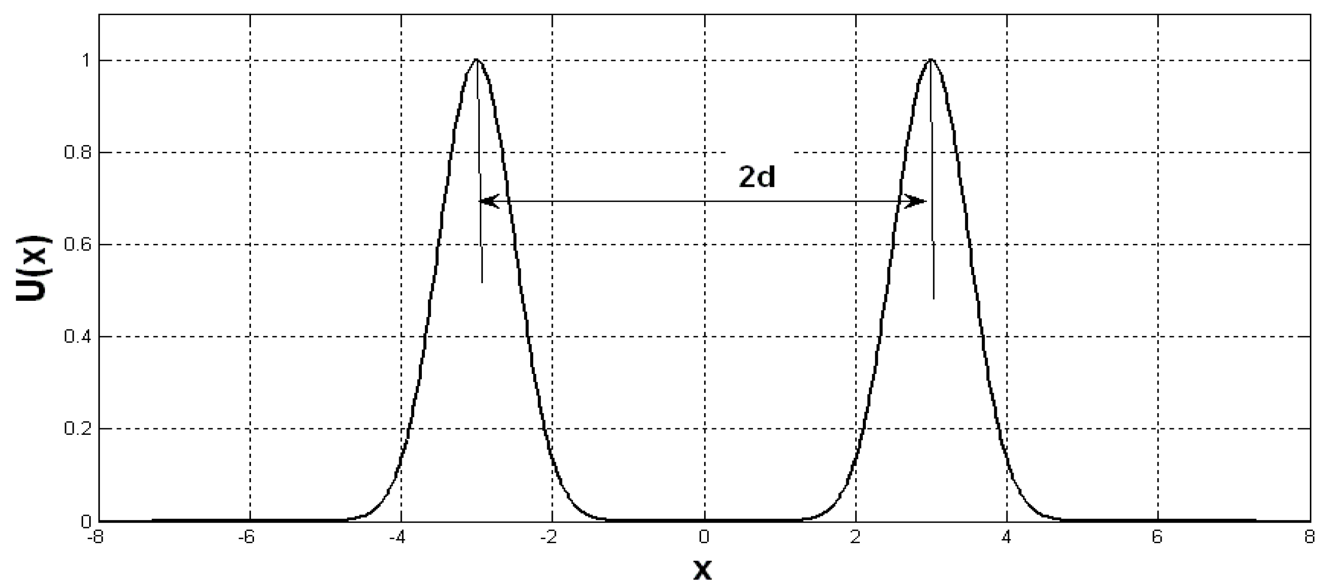
Abstract
:1. Introduction
2. Materials and Methods
2.1. The Schrödinger Differential Equation
2.2. The Integral Schrödinger Equation and Its Transformations
2.3. The Reflection Coefficient
3. Results
3.1. Determining the B(ω,k) Integral
3.2. The Double Potential Barrier
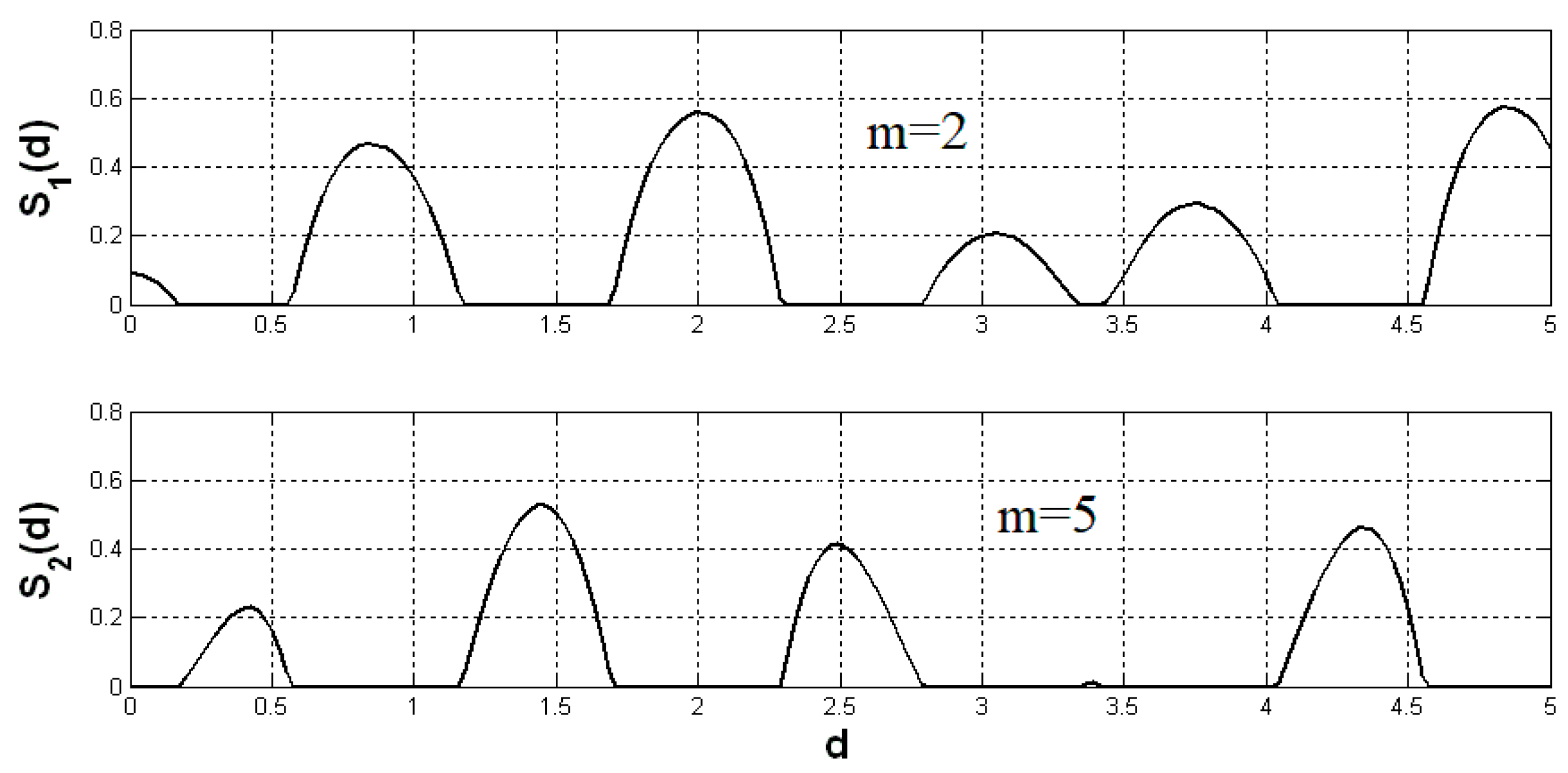
3.3. An Example of Calculations
4. Discussion
Author Contributions
Funding
Institutional Review Board Statement
Informed Consent Statement
Data Availability Statement
Acknowledgments
Conflicts of Interest
References
- Li, B.; Chen, Y.; Wang, Q. Exact analytical solutions to the nonlinear Schrödinger equation model. In Proceedings of the 2005 International Symposium on Symbolic and Algebraic Computation—ISSAC ’05, Beijing, China, 24–27 July 2005. [Google Scholar] [CrossRef]
- Belmonte-Beitia, J.; Gungor, F.; Torres, P.J. Explicit solutions with non-trivial phase of the inhomogeneous coupled two-component NLS system. J. Phys. A Math. Theor. 2020, 53, 015201. [Google Scholar] [CrossRef] [Green Version]
- Parwani, R.; Tabia, G. Universality in an information-theoretic motivated nonlinear Schrodinger equation. J. Phys. A Math. Theor. 2007, 40, 5621–5635. [Google Scholar] [CrossRef]
- Alhaidari, A.D. Analytic solution of the wave equation for an electron in the field of a molecule with an electric dipole moment. Ann. Phys. 2008, 323, 1709–1728. [Google Scholar] [CrossRef] [Green Version]
- Loboda, A.A. Schrödinger equation with signed Hamiltonian. Russ. J. Math. Phys. 2020, 27, 99–103. [Google Scholar] [CrossRef]
- Achilleos, V.; Diamantidis, S.; Frantzeskakis, D.J.; Karachalios, N.I.; Kevrekidis, P.G. Conservation laws, exact traveling waves and modulation instability for an extended nonlinear Schrödinger equation. J. Phys. A Math. Theor. 2015, 48, 355205. [Google Scholar] [CrossRef]
- Khawaja, U.A.; Al-Refai, M.; Shchedrin, G.; Carr, L.D. High-accuracy power series solutions with arbitrarily large radius of convergence for the fractional nonlinear Schrödinger-type equations. J. Phys. A Math. Theor. 2018, 51, 235201. [Google Scholar] [CrossRef]
- Syafwan, M.; Susanto, H.; Cox, S.M.; Malomed, B.A. Variational approximations for traveling solitons in a discrete nonlinear Schrödinger equation. J. Phys. A Math. Theor. 2012, 45, 075207. [Google Scholar] [CrossRef] [Green Version]
- Dmitriev, S.V.; Kevrekidis, P.G.; Yoshikawa, N.; Frantzeskakis, D.J. Exact stationary solutions for the translationally invariant discrete nonlinear Schrödinger equations. J. Phys. A Math. Theor. 2007, 40, 1727–1746. [Google Scholar] [CrossRef]
- Lashkin, V.M. N-soliton solutions and perturbation theory for the derivative nonlinear Schrödinger equation with nonvanishing boundary conditions. J. Phys. A Math. Theor. 2007, 40, 6119–6132. [Google Scholar] [CrossRef]
- Voros, A. Zeta-regularization for exact-WKB resolution of a general 1D Schrödinger equation. J. Phys. A Math. Theor. 2012, 45, 374007. [Google Scholar] [CrossRef]
- Musslimani, Z.H.; Makris, K.G.; El-Ganainy, R.; Christodoulides, D.N. Analytical solutions to a class of nonlinear Schrödinger equations with PT-like potentials. J. Phys. A Math. Theor. 2008, 41, 244019. [Google Scholar] [CrossRef]
- De Lima, E.F.; Ho, T.-S.; Rabitz, H. Solution of the Schrödinger equation for the Morse potential with an infinite barrier at long range. J. Phys. A Math. Theor. 2008, 41, 335303. [Google Scholar] [CrossRef]
- Silvestre-Brac, B.; Semay, C.; Buisseret, F. Auxiliary fields as a tool for computing analytical solutions of the Schrödinger equation. J. Phys. A Math. Theor. 2008, 41, 275301. [Google Scholar] [CrossRef] [Green Version]
- Edet, C.O.; Okoi, P.O.; Chima, S.O. Analytic solutions of the Schrödinger equation withnon-central generalized inverse quadratic Yukawa potential. Rev. Bras. de Ensino de Física 2020, 42, e20190083. [Google Scholar] [CrossRef] [Green Version]
- Akcay, H.; Sever, R. Analytical solutions of Schrödinger equation for the diatomic molecular potentials with any angular momentum. J. Math. Chem. 2012, 50, 1973–1987. [Google Scholar] [CrossRef]
- Abu-Shady, M. N-dimensional Schrödinger equation at finite temperature using the Nikiforov–Uvarov method. J. Egypt. Math. Soc. 2017, 25, 86–89. [Google Scholar] [CrossRef] [Green Version]
- Sacchetti, A. Solution to the double-well nonlinear Schrödinger equation with Stark-type external field. J. Phys. A Math. Theor. 2014, 48, 035303. [Google Scholar] [CrossRef]
- Manukyan, V.A.; Ishkhanyan, T.A.; Ishkhanyan, A.M. Schrödinger potential involving x2/3 and centrifugal-barrier terms conditionally integrable in terms of the confluent hypergeometric functions. Nonlinear Phenom. Complex Syst. 2019, 22, 84–92. [Google Scholar]
- Ishkhanyan, A.M.; Karwowski, J. The second Exton potential for the Schrödinger equation. Mod. Phys. Lett. A 2019, 34, 1950195. [Google Scholar] [CrossRef]
- Morse, P.M.; Feshbach, H. Methods of Theoretical Physics; McGraw-Hill Book Company, Inc.: New York, NY, USA; Toronto, ON, Canada; London, UK, 1953; Volume 1, 997p. [Google Scholar]
- Zhuravlev, V.F. Foundations of Theoretical Mechanics; Fizmatlit: Moscow, Russia, 2001; 321p. [Google Scholar]


Publisher’s Note: MDPI stays neutral with regard to jurisdictional claims in published maps and institutional affiliations. |
© 2021 by the authors. Licensee MDPI, Basel, Switzerland. This article is an open access article distributed under the terms and conditions of the Creative Commons Attribution (CC BY) license (https://creativecommons.org/licenses/by/4.0/).
Share and Cite
Bubenchikov, A.M.; Bubenchikov, M.A.; Chelnokova, A.S.; Jambaa, S. An Analytical Solution to the Problem of Hydrogen Isotope Passage through Composite Membranes Made from 2D Materials. Mathematics 2021, 9, 2353. https://doi.org/10.3390/math9192353
Bubenchikov AM, Bubenchikov MA, Chelnokova AS, Jambaa S. An Analytical Solution to the Problem of Hydrogen Isotope Passage through Composite Membranes Made from 2D Materials. Mathematics. 2021; 9(19):2353. https://doi.org/10.3390/math9192353
Chicago/Turabian StyleBubenchikov, Alexey Mikhailovich, Mikhail Alekseevich Bubenchikov, Anna Sergeevna Chelnokova, and Soninbayar Jambaa. 2021. "An Analytical Solution to the Problem of Hydrogen Isotope Passage through Composite Membranes Made from 2D Materials" Mathematics 9, no. 19: 2353. https://doi.org/10.3390/math9192353