
Statistical Inference for a General Family of Modified Exponentiated Distributions
by
 , , , and
Emilio Gómez-Déniz
1,† ,
,
Yuri A. Iriarte
2,†,
Yolanda M. Gómez
3,†,
Inmaculada Barranco-Chamorro
4,*,† and
Héctor W. Gómez
2,*,† 1
Department of Quantitative Methods in Economics and TiDES Institute, University of Las Palmas de Gran Canaria, 35017 Las Palmas de Gran Canaria, Spain
2
Departamento de Matemáticas, Facultad de Ciencias Básicas, Universidad de Antofagasta, Antofagasta 02800, Chile
3
Departamento de Matemáticas, Facultad de Ingeniería, Universidad de Atacama, Copiapó 1530000, Chile
4
Departamento de Estadística e Investigación Operativa, Facultad de Matemáticas, Universidad de Sevilla, 41012 Sevilla, Spain
*
Authors to whom correspondence should be addressed.
†
These authors contributed equally to this work.
Mathematics 2021, 9(23), 3069; https://doi.org/10.3390/math9233069
Submission received: 15 October 2021
/
Revised: 21 November 2021
/
Accepted: 24 November 2021
/
Published: 29 November 2021
Abstract
:In this paper, a modified exponentiated family of distributions is introduced. The new model was built from a continuous parent cumulative distribution function and depends on a shape parameter. Its most relevant characteristics have been obtained: the probability density function, quantile function, moments, stochastic ordering, Poisson mixture with our proposal as the mixing distribution, order statistics, tail behavior and estimates of parameters. We highlight the particular model based on the classical exponential distribution, which is an alternative to the exponentiated exponential, gamma and Weibull. A simulation study and a real application are presented. It is shown that the proposed family of distributions is of interest to applied areas, such as economics, reliability and finances.
1. Introduction
When the aim is to make inferences about a given real dataset, it is usually with statistics that the analyst starts the process of modeling, using classical distributions. Frequently, although a family of distributions seems appropriate, they do not provide a completely satisfactory description of the dataset, and there is a necessity to improve the model under consideration. In these cases, the chosen family of distributions can be considered as a starting point—it will be called the parent distribution—and the introduction of parameters may improve the statistical modeling process. It is well known that the incorporation of a new parameter into a baseline parametric model provides a new and more flexible one. For instance, it can be seen in [1] that the introduction of a scale parameter in the baseline hazard function resulted in accelerated failure time models, whereas taking powers of a baseline survival function yielded a proportional hazard model. The exponentiation method is quite general. Besides the previously mentioned hazard models, it is worth noting the max-stable family of distributions, whose cumulative distribution function (cdf) is obtained from a parent continuous cdf as
Equation (1) also present what is called the Lehmann alternatives; see [2,3]. An excellent review of the max-stable family of distributions along with a number of applications, mainly in the field of economics, can be found in [1]. It is also worth mentioning that, in reliability theory, the model given in (1) has been used used to describe random failure times. In this context, (1) is known as a proportional reversed hazard rate model. Relevant results on this topic, along with applications in reliability theory, can be seen in [4,5,6], and references therein. Other relevant papers related to (1) are: [7], where this model was used to provide a generalization of the classical logit and probit models; [8], wherein the authors related (1) to distributions of order statistics; and [9], wherein the authors introduced the generalized exponential distribution, which can be seen as a special case of the distribution introduced by Mudholkar et al. [10], and can be used as an alternative lifetime model to Gamma and Weibull distributions [11]. Estimation and other statistical inference issues in the generalized exponential distributions can be seen in [11,12,13,14,15,16]. We also wish to highlight the more recent paper by Jamal et al. [17], where a truncated general-G class of distributions is introduced, with emphasis on the truncated Burr-G family of distributions. The aim of our paper is to study and extend the family of distributions proposed in [17], which can also be considered as modified version of the family given in (1). We focus on properties which were not given by [17] and study in depth the special case of the sub-model exponential.
As for the merits of the max-stable distributions introduced in (1), which we aimed to keep in our proposal, we highlight
- A variety of shapes can be obtained due to the introduction of parameter .
- The random variable (rv) X with cdf F given in (1) can be obtained by applying a kind of inverse probability integral transformation (or alternatively ) to a distribution.
The class of distributions introduced in [17] also verifies these properties, with the difference that the truncated Burr-G family of distributions arises as a result of applying the inverse probability integral transformation to a truncated Burr distribution [17]. It will be shown that our proposal verifies a similar result and also allows us to obtain a variety of shapes in a continuous model, based on a modified exponentiation of the parent cdf.
The paper is organized as follows. In Section 2, the probability density function (pdf) for the new family of distributions is introduced, along with its genesis. The main properties of the family are given in Section 3. These are: the quantile function, random number generation, moments, ordering in terms of the shape parameter, Poisson mixture with our proposal as the mixing distribution (which can also be ordered), order statistics and tail behavior, with emphasis on cases in which heavy-tailed distributions are obtained. Section 4 is devoted to estimation methods: moment methods and maximum likelihood. The special case when the parent distribution is the classical exponential distribution is studied in Section 5. This model is referred to as the modified exponentiated exponential (MEE) distribution, and it is illustrated that can be used in reliability as an alternative to other lifetime models, in particular to the generalized exponential distribution proposed by Gupta and Kundu [9]. A simulation study is presented in Section 6. An application of the MEE model to a real dataset is provided in Section 7. To conclude, a brief discussion is given in Section 8. Throughout the paper, applications to economics, reliability and finance are included, which illustrate the potential uses of modified exponentiated distributions.
2. Materials and Methods
The next definition provides the cdf and the pdf of our proposal.
Definition 1.
Let Z be a continuous rv with cdf and pdf , where , , is a vector of unknown parameters. It is said that the rv Y is distributed according to a modified exponentiated family of distributions with parent cdf G, denoted as , with , if its cdf and pdf are given by
respectively, and .
Note that the support of agrees with the support of the parent distribution—that is, .
If , then the parent distribution, , is obtained.
For nonnegative rvs, from (2), the survival function is
from which we get the hazard rate function (hrf)
and the reversed hazard rate function is given by
Genesis of the Family
The family introduced in (2) can be related to the truncated Burr distribution and the general family of distributions proposed by [8], as we shall next see. Let
be the truncated in the pdf of a Burr (Type XII) or Singh–Maddala distribution (see [18]) with parameters and . It is well-known (see, for instance, [8]) that if is a continuous cdf with pdf , then we have that
is also the pdf of a continuous rv. Note that expression (3) can be obtained as a particular case of (7) by taking . Therefore, as is also the case with the max-stable distributions introduced in (1), the family (3) can be considered as the result of applying the inverse probability integral transformation to the one-parameter truncated on a (0, 1) Burr distribution, instead of a beta distribution. This property is of interest to get other properties, which involve the cdf, and generate random numbers in these models.
3. Results
The main results for this new family of distributions are given in this section.
3.1. Quantile Function and Random Number Generation
Proposition 1.
Let . Then the quantile function of Y is given by
where denotes the quantile function of the parent distribution G.
Proof.
Recall that the quantile function of Y is defined as
Expression (8) allows us to generate random numbers for the modified exponentiated family of distributions ME G by using the following algorithm:
- Generate .
- Compute .
3.2. Moments
Proposition 2.
Let . Then the moment of order r is given by
where is
being the quantile function associated with the parent distribution.
Proof.
Recall that
By making the change of variable , the result given in (9) is obtained. □
3.3. Stochastic Interpretation of the Parameters
Many parametric families of distributions can be ordered by using stochastic orders according to the values of their parameters. In this subsection we prove that the modified exponentiated family of distributions can be ordered with respect to the parameter in terms of the likelihood ratio, hazard rate and stochastic order, whose definitions can be seen, for example, in [19]. We highlight that this property can be of interest in applications of this model in disciplines such as insurance and reliability.
Definition 2.
Let and be continuous rvs with pdfs and , respectively, such that
Then is said to be smaller than in the likelihood ratio (LR) order, denoted by .
Proposition 3.
Let and . If , then .
Proof.
Let and . We have that
For ,
which implies that is decreasing on y. By applying Definition 2, Proposition 3 follows. □
It can be seen in [20] that the LR order is stronger than the hazard rate (HR) order, and in turn, this is stronger than stochastic (ST) order; that is,
Next we recall their definitions and some implications of this fact.
Definition 3.
Let and be two continuous rvs with hrfs and and cdfs and , respectively. Then
- 1.
- is said to be smaller than in the hazard rate order, denoted by if for all x.
- 2.
- is said to be stochastically smaller than , denoted by if for all x.
Corollary 1.
Let and . If , then
- 1.
- and .
- 2.
- .
Proof.
It is straightforward. □
Note that Corollary 1 implies that, for fixed values of , the mean of the parametric family of distributions increases with the values of the parameter .
3.4. Poisson-Modified Exponentiated Mixture
Mixtures of distributions constitute an interesting topic in applied statistics, especially in actuarial statistics. In the sequel we consider the mixture of a Poisson distribution with mean , denoted as , with a MEG distribution with positive support
Next it will be proven that (12) can be ordered. To reach this end, let be the cdf of the mixture Poisson–MEG distribution introduced in (12). The following result, analogous to Proposition 3, is established.
Proposition 4.
Let and be two Poisson–MEG mixtures with cdfs and , respectively. If , then .
Proof.
Let and be two MEG rvs with pdfs and , respectively. The cdf of the Poisson–MEG mixture with parameter , , is given by
where is the cdf of the Poisson rv with parameter , , .
Now, if , then, by applying Proposition 3, we have that
On the other hand, it is well-known (see, for example, Table 3.1 in [21]) that the Poisson model can also be ordered in terms of the likelihood ratio order
which is equivalent to say that the Poisson distribution of parameter is totally positive of order two (or TP2). Now Proposition 4 follows by applying Theorem 1.C.17 given in [20] (or alternatively, see Proposition 3.3.54 in [21]). □
Analogously to Corollary 1, the next result follows for the Poisson–MEG mixture, whose proof is omitted.
Corollary 2.
Let and be two Poisson–MEG mixtures with cdfs and and hrfs and , respectively. If then
- 1.
- and .
- 2.
- , for .
3.5. Order Statistics
Let be a random sample from a rv Y. If the rvs in the sample are arranged in increasing order of magnitude then the order statistics are obtained
In this series is the jth order statistic. Important cases of interest are the maximum, ; the minimum, ; and functions which involve the order statistics, such as the range, , the median and trimmed means, to name only a few.
The interest in order statistics to statistical inferences is twofold. On the one hand, they are building-block tools in nonparametric inference. On the other hand, they (and their functions) have relevant practical applications. They are used in the analysis of floods and droughts, reliability and fatigue failure, quality control, environmental and financial studies, among other fields. For all these reasons, some results are next given for the order statistics when sampling from a distribution.
First, recall that given a random sample from a continuous population, with cdf and pdf , the pdf of the jth order statistic, , is given by
for ; see [22]. Therefore, the pdf of the order statistics for a modified exponentiated distribution is
In particular, the pdf of the maximum is
and the pdf of the minimum, , is
A number of results related to order statistics can be deduced from previous pdfs. Other ones can be obtained from the properties of the family. As an illustration we give the next one, which establishes that the order statistics, and their expected values are also ordered in terms of the shape parameter .
Corollary 3.
Let and . If , then
- 1.
- for .
- 2.
- , provided the expectations exist.
Proof.
By applying Corollary 1, if , then . It can be seen in [22], Theorem 4.4.1, that implies the results given in 1 and 2. □
3.6. Right Tail Behavior
Important issues in distribution theory deal with long-tailed and heavy-right-tailed properties. These points are next studied. Their applications, mainly in financial and actuarial statistics, are also pointed out. Additional details can be seen in [23] and references therein. First, we recall that for a continuous rv X its cdf is , and the complementary event is
In survival and reliability analysis, (14) is referred to as the survival function, and it is usually denoted as . Contrarily, in economics, financial and actuarial statistics, (14) is usually denoted as and it is called the right tail of the cdf F; see [24]. Both nomenclatures are used throughout this paper, depending on the context.
The study of is related to the right tail behavior of the distribution: long tails, heavy tails and regular tails are analytical properties of interest, which we next study.
Lemma 1.
Let F be a continuous cdf. If
then F is long-tailed, and therefore F is also heavy-right-tailed; see [25].
Recall that if a distribution is heavy-right tailed, then its right tail is heavier than the exponential distribution. In the next proposition, conditions are given, in terms of the pdf of the parent distribution g, so that the distribution obtained as a result of applying (2) has a heavy right tail.
Proposition 5.
Let G be a continuous distribution such that its pdf g verifies that and tend to zero as . Then the family obtained by applying (2) is heavy-right-tailed.
Proof.
Let us consider . By applying the L’Hospital rule twice, and since it is supposed that and tend to zero as , we have that
From Lemma 1, the proposed result is obtained. □
An immediate consequence of Proposition 5 is given in the next corollary. This is, for a parent distribution verifying the conditions given in Proposition 5, the distribution has tails which are not exponentially bounded.
Corollary 4.
Under the conditions given in Proposition 5, it is verified that
Corollary 5.
Examples of heavy-right-tailed models.
- 1.
- Take , , the cdf of a Pareto distribution with shape parameter and scale parameter . Then the model is heavy-right-tailed.
- 2.
- Take , ; the cdf of a lognormal distribution with parameters and ; and Φ to denote the cdf of the standard normal distribution. Then the model is heavy-right-tailed.
Proof.
Both results follow from the application of Proposition 5. Since
- In this case and . Both functions tend to zero as , .
- In this case and , which tend to zero as .
□
An important issue in extreme value theory is the regular variation; see [26] or [27]. This property provides a flexible description of the variation of a given function according to a polynomial form of type , with . This idea is next formalized to study the right tail of a distribution.
Definition 4.
A cdf F is said to be regularly varying at infinity if there exits such that
δ is called the tail index.
The next theorem gives conditions on the parent distribution so that the cdf introduced in (2) has regular variation at ∞.
Proposition 6.
Let G be a continuous parent cdf such that its pdf verifies that , and . Then, the cdf introduced in (2) is regularly varying at ∞ with tail index δ.
Proof.
Let us consider the cdf given in (2). After applying the L’Hospital rule we get
Hence, the proposed result follows. □
An immediate consequence of Proposition 6 is given in Corollary 6. There, the notation as is used, which means that as ; see [24].
Corollary 6.
Let be independent and identically distributed as a nonnegative rv Y with the cdf given in (2) and . Then
Moreover, if then
Corollary 6 states that for a large y the event is due to the event . Therefore, exceedances of a high threshold by the sum are due to the exceedance of this threshold by the largest value in the sample.
Corollary 7.
If the parent distribution is a Pareto model with shape parameter and scale parameter , i.e., , , then the model obtained has regular variation at ∞.
Proof.
The result follows, since in this case . □
4. Inference
Let be a random sample from , where denotes the vector of unknown parameters associated with the parent distribution . Moment and maximum likelihood (ML) estimators for and are studied in this section.
4.1. Moment Estimators
By applying the method of moments,
with the sample moment of order j. From results given in Proposition 2, the moment estimator of , , is given as the solution of the system of equations
where was given in (10).
4.2. Maximum Likelihood Estimation
Given a random sample from the distribution , the log likelihood function is
where and are the pdf and cdf of the parent distribution with vector of unknown parameters . By taking the first partial derivatives in (16) with respect to for and , and setting them equal to zero, the log-likelihood equations are
where
In order to apply an iterative method of optimization, one of the equations given in (17) can be solved in , and we obtain
Now, by replacing in the remaining k equations, the ML estimates of the parameter can be obtained. The optim function available in the R package can be used in the maximization process. As initial values to start the process of estimation, the moment estimates can be used. Another option is to start with the MLEs of parameters in the parent distribution [28], , and to propose an initial from one of the equations in (17).
Under suitable conditions (regularity conditions) it is verified that the ML estimators of the parameters, properly normalized, converge in law to the standard normal distribution, , as n tends to infinity, which means that the asymptotic distribution of ML estimators can be approached for a normal distribution as n is large.
5. A Relevant Sub-Model: The Exponential Case
In this section, we consider the particular case in which the parent distribution G corresponds to an exponential model with rate parameter , . First, the submodel is defined; later, new and relevant properties are listed.
Definition 5.
An rv Y follows a modified exponentiated exponential (MEE) distribution, , if its pdf is given by
Here, and are the rate and shape parameters, respectively. Obviously, if , then the reduces to the classical exponential distribution, .
Proposition 7.
Let . Then
- 1.
- The hazard function is
- 2.
- The moment generating function of Y iswhere denotes the incomplete beta function; is defined for , ; and .
- 3.
- The expected value of Y can be obtained aswhereis the generalized hypergeometric function.
Proof.
1. It is immediate as result of applying (5).
2. From (19)
By making the change of variable in (23) and taking into account the definition of the incomplete beta function, (21) is obtained.
3. From (21), is obtained as the first derivative with respect to t of and by setting , which, in turn, can be written in terms of the generalized hypergeometric function. To get (22), we need the derivative of the incomplete beta function (see The Wolfram functions site https://functions.wolfram.com (accessed on 25 September 2021)), which is given by
Furthermore, the following relationship is used:
□
Shape of Distribution
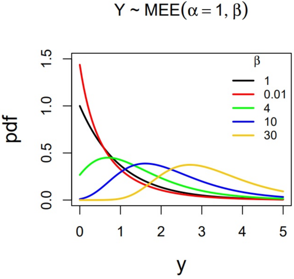
Since is a rate parameter, without loss of generality it can be , and the shape of the distribution can be studied in terms of . Figure 1 and Figure 2 show some plots of the pdf and hrf for different values of the shape parameter. The cases (red color), (black color) and (green, blue and yellow colors) are considered.
In these figures we can observe that for , the pdf is monotically decreasing, and the hazard rate too. Moreover, for , the hazard rate approaches one when y tends to . For , recall that the classical exponential distribution is obtained; its pdf is plotted in black in Figure 1, and its hazard rate is the constant one (black) in Figure 2. On the other hand, for , it can be seen in Figure 1 that the pdf is strongly unimodal and the hazard rate function is monotically increasing, approaching one when y tends to . As was proven in Section 3.3, these families of distributions are ordered in terms of hazard rate. This fact is clearly appreciated in Figure 2. These comments are formalized next.
Remark 1.
In this context, the term strongly unimodal means that the pdf f reaches its maximum at m, an interior point in the support of the distribution, and there are no other local maxima.
Proposition 8
(Shape of the pdf and hrf in the distribution).
- 1.
- For any , it is verified that if , then is monotically decreasing and its mode is at zero. On the other hand, if , then is strongly unimodal and the mode is at , where denotes natural logarithm.
- 2.
- For any , it is verified that if , then the hrf, , is monotically decreasing; if , then the hrf is constant, ; and if , then is monotically increasing.Moreover,
Proof.
Recall that a function f is log-concave if and only if
A number of properties can be deduced in the distribution from (25).
Proposition 9.
If , then the pdf of the distribution is log-concave, and if , then it is log-convex.
Proof.
Recall that if for all y, then f is log-concave. Analogously, if it is , then f is log-convex.
Since in this case
the result proposed follows. □
Immediate consequences are listed in the following corollary.
Corollary 8.
Let . Then
- 1.
- If (), then the cdf and survival functions are log-concave (log-convex).
- 2.
- If , then the truncated distribution at , , is also log-concave.
Proof.
These properties follow from the log-concavity (log-convexity) of the pdf; see, for instance, [29]. □
Other properties, such as the hazard rate function monotonically increasing for and monotonically decreasing for , can also be deduced from Proposition 9. They are omitted in Corollary 8 because they were previously proven in Proposition 8.
Remark 2
(Application of (24) of interest in reliability). As interesting applications of properties given in this subsection, we highlight the result given in (24) for . In this case we have a lifetime model whose hazard function increases from zero to a finite constant, . Gupta and Kundu [12] pointed out that this kind of model can be appropriate for describing a population of items which are in a regular maintenance program. That is, the hazard rate increases initially, but after some time the system reaches a stable situation due to maintenance.
Next, the quantile function of distribution is given along with a simulation study, which illustrates the use of this function. Applications of interest in reliability and finance are also listed.
Corollary 9.
Let . Then the quantile function obtained from (8) is
The algorithm proposed in Section 3.1 along with (26) can be applied to obtain simulated values of the distribution. Figure 3 shows the histogram for a simulated dataset of size by using that algorithm with and . We highlight the good agreement between the histogram and the pdf of this model.
Remark 3
(Practical applications of quantiles). We can cite
- 1.
- In reliability and survival analysis, models such as the distribution are of interest. In this context, quantiles are used to establish warranty periods of products, for modeling lifetime data, and to estimate features in the model not affected by the presence of outliers. The parametric estimation of quantiles tends to be more efficient than nonparametric estimation, as can be seen in [30].
- 2.
- In financial and actuarial theory, the quantile function is also known as the value at risk, (denoted as VaR), which is interpreted as the amount of capital required to ensure that the insurer (or the economic agent) does not become insolvent with a high degree of certainty. Therefore, it is of interest to have an explicit expression for this function, such as the one given in (26). This measure is also of great importance in scenarios where outliers corresponding to large empirical data may appear, which is quite common in risk theory. In this sense, we highlight that the MEE distribution seems appropriate for modeling this kind of empirical data, as can be seen in Figure 3.
To conclude this section, expressions for the moments are given.
Corollary 10.
Let . Then the moment of order r is given by
where and .
6. Simulation Study
In order to study the performance of the estimators obtained by the ML method, a simulation study was carried out. We focused on the relevant model introduced in Section 5 with only two parameters, and . One thousand samples of sizes were generated from the MEE model for several values of the parameters. The random numbers were generated by using the algorithm introduced in the Section 3.1.
Summaries of these simulations are given: the means of the estimates and their standard errors (s.e.) in parentheses.
Results in Table 1 suggest that
- The ML estimators were biased, but the bias tended to zero when n increased.
- The standard deviation of the estimates decreased when the sample size n increased.
- Since the previous summaries tended to zero if n increased, both estimators seem to have been consistent. That is, if , then closer estimates to the true values of the parameters were obtained.
- It can be appreciated that, for the values of the parameters and the sample sizes under consideration, the bias and standard deviation of are greater than the bias and standard deviation of , but in any case, both estimators exhibited good behavior, since if n increased, then both summaries decreased.
7. Application
An application with a real dataset was carried out. We proved that our proposal outperforms other common two-parameter lifetime distributions that can appropriately fit reliability data.
Modeling of a Fatigue Fracture in Kevlar 373/Epoxy Data
In this application a set of data were fitted by using the distribution. We proved that this model can be considered as an alternative to the Weibull and generalized exponential distributions introduced by Gupta and Kundu [9]. All these models had the same number of parameters and contained, in one particular case, the one-parameter exponential distribution. Recall that the Weibull and generalized exponential pdfs are given by
- 1.
- Weibull, , distribution:
- 2.
- Generalized exponential, , distribution:
In this application we compared the performances of the MEE, Weibull, generalized exponential and exponential distributions.
The dataset consisted of the lifetimes of fatigue fractures of Kevlar 373/epoxy, which were subject to constant pressure at the 90% stress level until all of them failed. Thus, we had complete data with the exact times of failure. This dataset can be seen in Table 2.
This dataset has been analyzed by a number of authors; see, for instance, [31,32]. The descriptive summaries are given in Table 3: sample mean, sample standard deviation, and (the latter are the sample asymmetry and kurtosis coefficients, respectively).
By using the results given in Section 4.1, moment estimators were computed, leading to the following estimates: = 0.7329 and = 3.6316, which were used as initial estimates for the ML approach. Table 4 shows the parameter estimates (with their standard errors in parenthesis) for MEE, GE, W and exponential (E) distributions obtained by using the ML method.
In order to compare the distributions, the Akaike information criterion (AIC) introduced by Akaike [33] and the Bayesian information criterion (BIC) proposed by Schwarz [34] were used. It is well known that AIC and BIC , where k is the number of parameters in the model, n is the sample size and is the maximized value of the log-likelihood function. Table 5 shows the corresponding AIC and BIC for each model. From these criteria, the better fit was provided by the MEE model. Figure 4 gives the histogram for the data along with the fitted densities, where the good fit provided by the MEE distribution can be seen.
8. Discussion
In this paper, a general class of modified exponentiated distributions has been introduced. The building-block is the modified exponentiation of the cdf of a parent distribution denoted by G. Properties of this new family of distributions were obtained in terms of G and the exponent, which acts as a shape parameter on the parent distribution. First, the general properties were obtained. These are: the cdf, pdf, quantile function, moments, order statistics and heavy tail properties, among others. It was shown that the family exhibits more flexible behavior than the parent distribution, and therefore it is suitable for fitting data of diverse nature. In order to interpret the shape parameter, stochastic orders are considered. We highlighted that some of these properties, such as the Poisson-modified exponentiated mixture and heavy tail behavior, are important due to their involvement in actuarial statistics. Other properties, such as those related to quantiles, hazard and survival function, are of interest in reliability and survival analysis. As estimation methods, moment and maximum likelihood methods have been proposed. As a particular case of interest, we used as the parent distribution the classical exponential distribution and obtained the MEE model. For this submodel, new properties were obtained, which show that MEE model can be an efficient alternative to Weibull and generalized exponential distributions for analyzing lifetime data. A simulation study was included, which illustrated the performance of ML estimators. Finally, a real application was presented, which shows that the new family can be a competitor of two-parameter distributions that receive common use in statistics and reliability. Immediate extensions of this work would allow one to obtain the modified exponentiated Pareto distribution, which should be of interest for economic and actuarial problems, and their multivariate generalizations. Some of the merits of this future research have been pointed out in the particular cases of parent distributions studied in Section 3.6.
Author Contributions
Conceptualization, E.G.-D.; formal analysis, I.B.-C.; investigation, Y.A.I. and Y.M.G.; supervision, H.W.G. All authors have read and agreed to the published version of the manuscript.
Funding
The research of H.W.G. was funded by SEMILLERO UA-2021 (Chile). E.G.-D. was partially funded by grant ECO2013–47092 (Ministerio de Economía y Competitividad, Spain) and ECO2017–85577–P (Ministerio de Economía, Industria y Competitividad. Agencia Estatal de Investigación).
Data Availability Statement
The real dataset under study is included in the paper.
Acknowledgments
Authors want to thanks the referees for the careful reading of the paper and their helpful comments, which contribute to improve it. The research of H.W.G. was supported by SEMILLERO UA-2021 (Chile). E.G.-D. was partially funded by grant ECO2013–47092 (Ministerio de Economía y Competitividad, Spain) and ECO2017–85577–P (Ministerio de Economía, Industria y Competitividad. Agencia Estatal de Investigación). The authors want to express their gratitude for these supports.
Conflicts of Interest
The authors declare no conflict of interest.
Abbreviations
The following abbreviations are used in this manuscript:
| cdf | cumulative distribution function |
| rv | random variable |
| probability density function | |
| hrf | hazard rate function |
| MEG | modified exponentiated family with parent cdf G |
| MEE | modified exponentiated exponential model |
| W | Weibull |
| GE | generalized exponential |
| E | (classical) Exponential distribution |
| ML | maximum likelihood |
References
- Sarabia, J.; Castillo, E. About a Class of Max-Stable Families with Applications to Income Distributions. Metron 2005, LXIII, 505–527. [Google Scholar]
- Lehmann, E. The power of rank test. Ann. Math. Stat. 2007, 24, 23–43. [Google Scholar] [CrossRef]
- Gupta, R.; Gupta, P.; Gupta, R. Modeling failure time data by Lehmann alternatives. Commun. Stat.-Theory Methods 1998, 27, 887–904. [Google Scholar] [CrossRef]
- Di Crescenzo, A. Some results on the proportional reversed hazards model. Stat. Probab. Lett. 2000, 50, 313–321. [Google Scholar] [CrossRef]
- Gupta, R.C.; Gupta, R.D. Proportional reversed hazard rate model and its applications. J. Stat. Plan. Inference 2007, 137, 3525–3536. [Google Scholar] [CrossRef]
- Sankaran, P.; Gleeja, V. Proportional reversed hazard and frailty models. Metrika 2008, 68, 333–342. [Google Scholar] [CrossRef]
- Prentice, R. A generalization of the probit and logit methods for dose–response curves. Biometrika 1976, 32, 761–768. [Google Scholar] [CrossRef]
- Jones, M. Families of distributions arising from distributions of order statistics. Test 2004, 13, 1–43. [Google Scholar] [CrossRef]
- Gupta, R.; Kundu, D. Generalized Exponential Distributions. Aust. N. Z. J. Stat. 1999, 41, 173–188. [Google Scholar] [CrossRef]
- Mudholkar, G.; Srivastava, D.; Freimer, M. The exponentiated Weibull Family—A reanalysis of the Bus-Motor-Failure data. Technometrics 1995, 37, 436–445. [Google Scholar] [CrossRef]
- Gupta, R.; Kundu, D. Generalized Exponential Distributions: Different Methods of Estimation. J. Stat. Comput. Simul. 2018, 69, 315–338. [Google Scholar] [CrossRef]
- Gupta, R.; Kundu, D. Exponentiated Exponential Family: An Alternative to Gamma and Weibull. Biom. J. 2001, 33, 117–130. [Google Scholar] [CrossRef]
- Gupta, R.; Kundu, D. Generalized Exponential Distribution: Statistical Inferences. J. Stat. Theory Appl. 2002, 1, 101–118. [Google Scholar]
- Gupta, R.; Kundu, D. Generalized exponential distribution: Existing results and some recent developments. J. Stat. Plan. Inference 2007, 137, 3537–3547. [Google Scholar] [CrossRef] [Green Version]
- Mitra, S.; Kundu, D. Analysis of the left censored data from the generalized exponential distribution. J. Stat. Comput. Simul. 2008, 78, 669–679. [Google Scholar] [CrossRef]
- Gupta, R.; Kundu, D. Generalized exponential distribution: Bayesian Inference. Comput. Stat. Data Anal. 2008, 52, 1873–1883. [Google Scholar]
- Jamal, F.; Bakouch, H.; Nasir, A. A truncated general-G class of distributions with application to truncated Burr-G family. Revstat.-Stat. 2020. to appear. [Google Scholar]
- Burr, I. Cumulative frequency functions. Ann. Math. Stat. 1942, 13, 215–232. [Google Scholar] [CrossRef]
- Ross, S. Stochastic Processes, 2nd ed.; John Wiley & Sons, Inc.: Hoboken, NJ, USA, 1996. [Google Scholar]
- Shaked, M.; Shanthikumar, J. Stochastic Orders; Series: Springer Series in Statistics; Springer: New York, NY, USA, 2007. [Google Scholar]
- Denuit, M.; Goovaerts, M.; Kaas, R. Actuarial Theory for Dependent Risks; John Wiley & Sons: Hoboken, NJ, USA, 2005. [Google Scholar]
- David, H.A.; Nagaraja, H.N. Order Statistics, 3rd ed.; John Wiley & Sons: Hoboken, NJ, USA, 2003. [Google Scholar]
- Gómez-Déniz, E.; Calderín-Ojeda, E. Financial and actuarial properties of the Beta-Pareto as a long-tail distribution. Span. J. Stat. 2020, 2, 7–21. [Google Scholar] [CrossRef]
- Jessen, A.; Mikosch, T. Regularly varying functions. Publ. L’institut Mathématique. Nouv. Ser. 2006, 80, 171–192. [Google Scholar] [CrossRef]
- Rolski, T.; Schimidli, H.; Schmidt, V.; Teugels, J. Stochastic Processes for Insurance & Finance; John Wiley & Sons, Ltd.: Hoboken, NJ, USA, 1999. [Google Scholar]
- Bingham, N.; Goldie, C.; Teugels, J. Regular Variation; Cambridge University Press: Cambridge, UK, 1987. [Google Scholar]
- Konstantinides, D. Risk Theory: A Heavy Tail Approach; World Scientific: Singapore, 2018. [Google Scholar]
- Martínez-Flórez, G.; Barranco-Chamorro, I.; Gómez, H.W. Flexible Log-Linear Birnbaum–Saunders Model. Mathematics 2021, 9, 1188. [Google Scholar] [CrossRef]
- Bagnoli, M.; Bergstrom, T. Log-Concave Probability and Its Applications. Econ. Theory 2005, 26, 445–469. [Google Scholar] [CrossRef] [Green Version]
- Barranco-Chamorro, I.; Jiménez-Gamero, M.D. Asymptotic results in partially non-regular log-exponential distributions. J. Stat. Comput. Simul. 2012, 82, 445–461. [Google Scholar] [CrossRef]
- Andrews, D.; Herzberg, A. Data: A Collection of Problems from Many Fields for the Student and Research Worker; Springer Series in Statistics; Springer: New York, NY, USA, 1985. [Google Scholar]
- Barlow, R.; Toland, R.; Freeman, T. A Bayesian analysis of stress-rupture life of kevlar 49/epoxy spherical pressure vessels. In Proceedings of the Conference on Applications of Statistics; Marcel Dekker: New York, NY, USA, 1984. [Google Scholar]
- Akaike, H. A new look at the statistical model identification. IEEE Trans. Autom. Control 1974, 19, 716–723. [Google Scholar] [CrossRef]
- Schwarz, G. Estimating the dimension of a model. Ann. Stat. 1978, 6, 461–464. [Google Scholar] [CrossRef]
Figure 1.
Plots of the MEE distribution pdf for different values of parameter .

Figure 2.
Plots of the hrf of MEE for different values of parameter .

Figure 3.
Histogram for the simulated study with size for MEE distribution.

Figure 4.
Models fitted by the ML approach to the Kevlar 373/epoxy dataset.


Table 1.
Means and standard errors (s.e.) for the estimates obtained by ML in the MEE distribution.
| MEE | |||||||
|---|---|---|---|---|---|---|---|
| (s.e.) | (s.e.) | (s.e.) | (s.e.) | (s.e.) | (s.e.) | ||
| 3 | 2 | 3.150 (1.120) | 2.038 (0.363) | 3.084 (0.845) | 2.036 (0.257) | 3.070 (0.627) | 2.022 (0.191) |
| 4 | 4.154 (1.205) | 2.046 (0.325) | 4.117 (0.895) | 2.027 (0.245) | 4.050 (0.650) | 2.013 (0.163) | |
| 5 | 5.204 (1.230) | 2.043 (0.296) | 5.152 (0.963) | 2.026 (0.206) | 5.056 (0.696) | 2.010 (0.155) | |
| 10 | 5 | 10.743 (2.697) | 5.123 (0.668) | 10.426 (1.851) | 5.087 (0.455) | 10.163 (1.214) | 5.023 (0.316) |
| 10 | 10.627 (2.589) | 10.207 (1.248) | 10.346 (1.751) | 10.109 (0.864) | 10.136 (1.133) | 10.058 (0.624) | |
| 15 | 10.674 (2.449) | 15.350 (1.851) | 10.366 (1.824) | 15.225 (1.368) | 10.270 (1.218) | 15.146 (0.933) | |
| 3 | 3 | 3.255 (1.305) | 3.123 (0.580) | 3.137 (0.895) | 3.071 (0.398) | 3.071 (0.604) | 3.023 (0.271) |
| 4 | 4 | 4.241 (1.366) | 4.129 (0.695) | 4.107 (0.942) | 4.043 (0.490) | 4.065 (0.640) | 4.041 (0.342) |
| 5 | 5 | 5.291 (1.538) | 5.132 (0.791) | 5.138 (0.972) | 5.085 (0.544) | 5.019 (0.707) | 5.005 (0.389) |
Table 2.
Data corresponding to the real application.
| 0.0251 | 0.0886 | 0.0891 | 0.2501 | 0.3113 | 0.3451 | 0.4763 | 0.5650 |
| 0.5671 | 0.6566 | 0.6748 | 0.6751 | 0.6753 | 0.7696 | 0.8375 | 0.8391 |
| 0.8425 | 0.8645 | 0.8851 | 0.9113 | 0.9120 | 0.9836 | 1.0483 | 1.0596 |
| 1.0773 | 1.1733 | 1.2570 | 1.2766 | 1.2985 | 1.3211 | 1.3503 | 1.3551 |
| 1.4595 | 1.4880 | 1.5728 | 1.5733 | 1.7083 | 1.7263 | 1.7460 | 1.7630 |
| 1.7746 | 1.8275 | 1.8375 | 1.8503 | 1.8808 | 1.8878 | 1.8881 | 1.9316 |
| 1.9558 | 2.0048 | 2.0408 | 2.0903 | 2.1093 | 2.1330 | 2.2100 | 2.2460 |
| 2.2878 | 2.3203 | 2.3470 | 2.3513 | 2.4951 | 2.5260 | 2.9911 | 3.0256 |
| 3.2678 | 3.4045 | 3.4846 | 3.7433 | 3.7455 | 3.9143 | 4.8073 | 5.4005 |
| 5.4435 | 5.5295 | 6.5541 | 9.0960 |
Table 3.
Statistical summaries for fatigue data of Kevlar 373/epoxy.
| n | s | |||
|---|---|---|---|---|
| 76 | 1.959 | 1.574 | 1.979 | 8.161 |
Table 4.
ML estimates of the fitted models with their respective standard errors (s.e.).
| Parameters Estimated | MEE (s.e.) | GE (s.e.) | W (s.e.) | E (s.e.) |
|---|---|---|---|---|
| 4.807 (1.120) | 1.709 (0.282) | 1.325 (0.113) | - | |
| 0.831 (0.106) | 0.702 (0.092) | 2.132 (0.194) | 0.510 (0.058) |
Table 5.
Akaike information criterion and Bayes information criterion for every model.
| Criterion | MEE | GE | W | E |
|---|---|---|---|---|
| AIC | 246.3844 | 248.4872 | 249.0494 | 256.2286 |
| BIC | 251.0459 | 253.1487 | 253.7109 | 258.5593 |
Publisher’s Note: MDPI stays neutral with regard to jurisdictional claims in published maps and institutional affiliations. |
© 2021 by the authors. Licensee MDPI, Basel, Switzerland. This article is an open access article distributed under the terms and conditions of the Creative Commons Attribution (CC BY) license (https://creativecommons.org/licenses/by/4.0/).
Share and Cite
MDPI and ACS Style
Gómez-Déniz, E.; Iriarte, Y.A.; Gómez, Y.M.; Barranco-Chamorro, I.; Gómez, H.W. Statistical Inference for a General Family of Modified Exponentiated Distributions. Mathematics 2021, 9, 3069. https://doi.org/10.3390/math9233069
AMA Style
Gómez-Déniz E, Iriarte YA, Gómez YM, Barranco-Chamorro I, Gómez HW. Statistical Inference for a General Family of Modified Exponentiated Distributions. Mathematics. 2021; 9(23):3069. https://doi.org/10.3390/math9233069
Chicago/Turabian StyleGómez-Déniz, Emilio, Yuri A. Iriarte, Yolanda M. Gómez, Inmaculada Barranco-Chamorro, and Héctor W. Gómez. 2021. "Statistical Inference for a General Family of Modified Exponentiated Distributions" Mathematics 9, no. 23: 3069. https://doi.org/10.3390/math9233069
Note that from the first issue of 2016, this journal uses article numbers instead of page numbers. See further details here.