
Flexible Power-Normal Models with Applications
by
 , , ,
, , ,
Guillermo Martínez-Flórez
1 ,
,
Diego I. Gallardo
2,
Osvaldo Venegas
3,*,
Heleno Bolfarine
4 and
Héctor W. Gómez
5 1
Departamento de Matemáticas y Estadística, Facultad de Ciencias, Universidad de Córdoba, Córdoba 2300, Colombia
2
Departamento de Matemática, Facultad de Ingeniería, Universidad de Atacama, Copiapó 1530000, Chile
3
Departamento de Ciencias Matemáticas y Físicas, Facultad de Ingeniería, Universidad Católica de Temuco, Temuco 4780000, Chile
4
Departamento de Estatística, IME, Universidade de São Paulo, São Paulo 05508-090, Brazil
5
Departamento de Matemáticas, Facultad de Ciencias Básicas, Universidad de Antofagasta, Antofagasta 1240000, Chile
*
Author to whom correspondence should be addressed.
Mathematics 2021, 9(24), 3183; https://doi.org/10.3390/math9243183
Submission received: 18 November 2021
/
Revised: 2 December 2021
/
Accepted: 6 December 2021
/
Published: 10 December 2021
(This article belongs to the Section Probability and Statistics)
Abstract
:The main object of this paper is to propose a new asymmetric model more flexible than the generalized Gaussian model. The probability density function of the new model can assume bimodal or unimodal shapes, and one of the parameters controls the skewness of the model. Three simulation studies are reported and two real data applications illustrate the flexibility of the model compared with traditional proposals in the literature.
1. Introduction
Azzalini [1] introduced the skew-normal (SN) model and Durrans [2] introduced the generalized Gaussian model, also known as the power-normal (PN) model. A limitation of those models is that they only produce uni-modal asymmetric densities, and are therefore not appropriate for fitting bimodal data. An approach typically used for fitting multimodal data is the mixture of normal or asymmetric-normal models, which present difficulties such as identifiability problems (see McLachlan and Peel [3]; Marin et al. [4]) and complicated numerical implementation. Bimodal distributions generated from skew-symmetric distributions can be found in Azzalini and Capitanio [5], Ma and Genton [6], Arellano-Valle et al. [7], Kim [8], Lin et al. [9,10], Elal-Olivero et al. [11], Arnold et al. [12,13], Gómez et al. [14], Braga et al. [15], Venegas et al. [16] and Gómez-Déniz et al. [17], among others.
It is therefore of interest to study asymmetric models that are adequate for fitting possible bimodal data. Hence, the main object of this paper is to propose asymmetric distributions that are more flexible than the SN and PN models; and are also useful for modeling bimodal data, which are very common in practical situations. The proposed model is not a mixture type model, to avoid the identifiability problems mentioned above. Our proposal considers a family of distributions which can adopt both a unimodal shape (competing with the SN and PN models) and a bimodal shape (competing with the mixture of normals).
The following Lemma is introduced in Gómez et al. [14], and is crucial for the construction of the new family of distributions.
Lemma 1.
Let f be a symmetric around zero probability density function (pdf), F its respective cumulative distribution function (cdf) and G an absolutely continuous cdf such that is a symmetric pdf around zero. Then,
is the pdf of a random variable, where .
Gómez et al. [14] studied the skew-flexible-normal (SFN) distribution with pdf given by:
The authors show that, for , the model in (2) is bimodal. We denote this model as SFN().
The “Lehmann’s alternatives” model proposed in Lehmann [18] is based on the distribution of the maximum of a sample. It is a good alternative for extending models because it incorporates a higher asymmetry and/or kurtosis than the basal model. The cdf of this model is given by:
where F is a cdf. For , the cdf corresponds to the random variable defined as , where the s are independent and identically distributed with common cdf F. Durrans [2] extends this interpretation to fractional order statistics for . We denote a random variable with cdf defined in (3) as Z ∼ . The case, , corresponds to the PN model with pdf given by
which we denote by Z ∼ . This model has been studied in more detail in Gupta and Gupta [19]. Pewsey et al. [20] derived its Fisher information matrix, showing that it is non-singular in a neighborhood of symmetry point (), which is not satisfied for the SN distribution under the symmetry hypothesis, that is, at , because its Fisher information matrix is singular.
The paper is organized as follows. In Section 2, the flexible power-normal (FPN) model is introduced and some of its main properties are discussed. An inference of the model via maximum likelihood (ML) estimation is considered in Section 3. Three procedures to draw values from the FPN distribution are discussed in Section 4. Three simulation studies are carried out in Section 5 in order to assess different aspects of the model. Two real data applications are reported in Section 6, illustrating the usefulness of the model compared with other common distributions in the literature. Finally, Section 7 presents a discussion of the main results of the paper.
2. Flexible Power-Normal Distribution
In this section, we introduce a more flexible model than the power-normal model introduced in (4) by incorporating a new shape parameter One of the interesting features of this model is that, for certain values of shape parameter , a bimodal pdf can be obtained.
Definition 1.
A random variable Z follows a FPN distribution with parameters α and δ, if its pdf is given by:
where
is the normalizing constant. We use the notation .
2.1. Some Particular Cases of the FPN Model
For the FPN distribution, we have the following particular cases.
Proposition 1.
If , then
- .
- .
- .
- .
Remark 1.
Note that points 1 and 2 show that N and PN distributions are particular cases of the FPN model. Points 3 and 4 show that the model contains particular cases of the skew-normal and skew-flexible-normal models (SN(1) and SFN(1,δ), respectively).
2.2. Properties of the pdf for the FPN Model
The following propositions illustrate a point where the pdf of the FPN model is not differentiable.
Proposition 2.
Let . If , then the pdf of the FPN is not differentiable at .
Proof.
Note that
from which we conclude that the pdf of the FPN model is not differentiable at as long as . □
Proposition 3.
Let . If , the distribution of the random variable Z is bimodal.
Proof.
Equating to zero the first derivative for the pdf of the random variable Z with FPN distribution, we have the following cases:
- If , then it follows that the solution is given by .
- If , we have the solution .
Moreover, if , and if , Hence, and are distinct values. Therefore, Z is a random variable with a bimodal distribution. □
Corollary 1.
Let . If and , then random variable Z is symmetric and bimodal.
Proof.
If then , . As is a symmetric function, we conclude that Z is a symmetric random variable. □
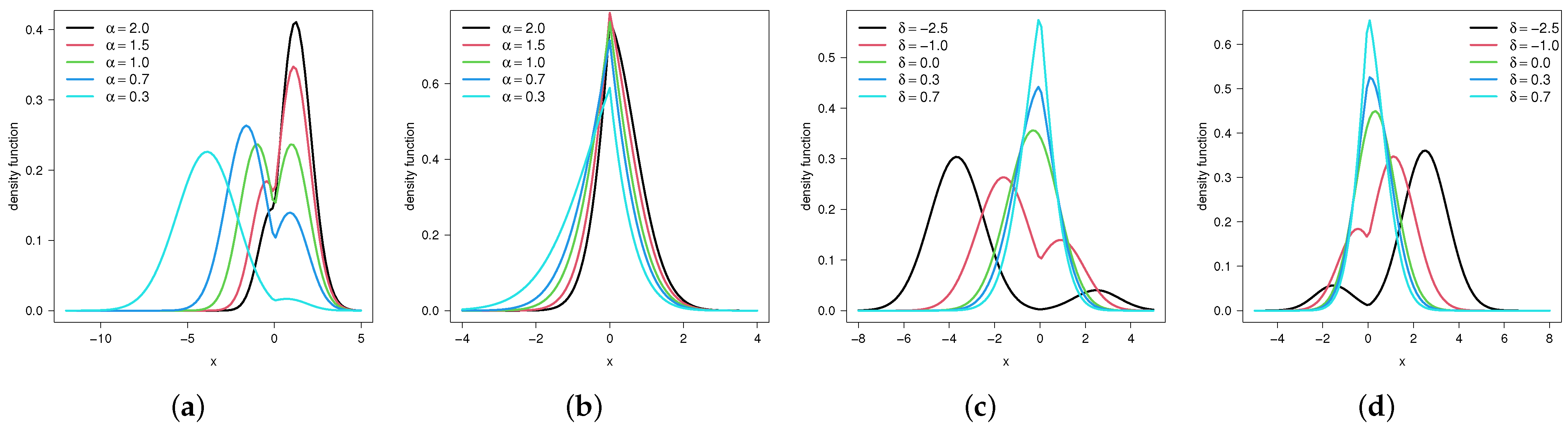
Figure 1 shows plots of the pdf for the FPN for different values of and . As mentioned previously, for a bimodal pdf is obtained, but one of the modes “disappears” when moves away from one ( or ), whereas for a unimodal pdf is obtained with different degrees of kurtosis (leptokurtic, mesokurtic or platykurtic) depending on the value of . On the other hand, and produce a positive and negative skew effect in the pdf, respectively, whereas corresponds to a symmetrical pdf.
2.3. Moments
Definition 2.
Let . For , we define the lower and upper r-th incomplete moments of Z as
respectively. With those definitions, the r-th moment of Z is given by
The next result presents a recursive expression for computing the moments of the FPN random variable.
Proposition 4.
Let . The r-th moment of the random variable Z is given by:
The r-th central moment, say , for , can be computed using the expressions:
, and
With those definitions, the variance and the asymmetry and kurtosis coefficients are given by:
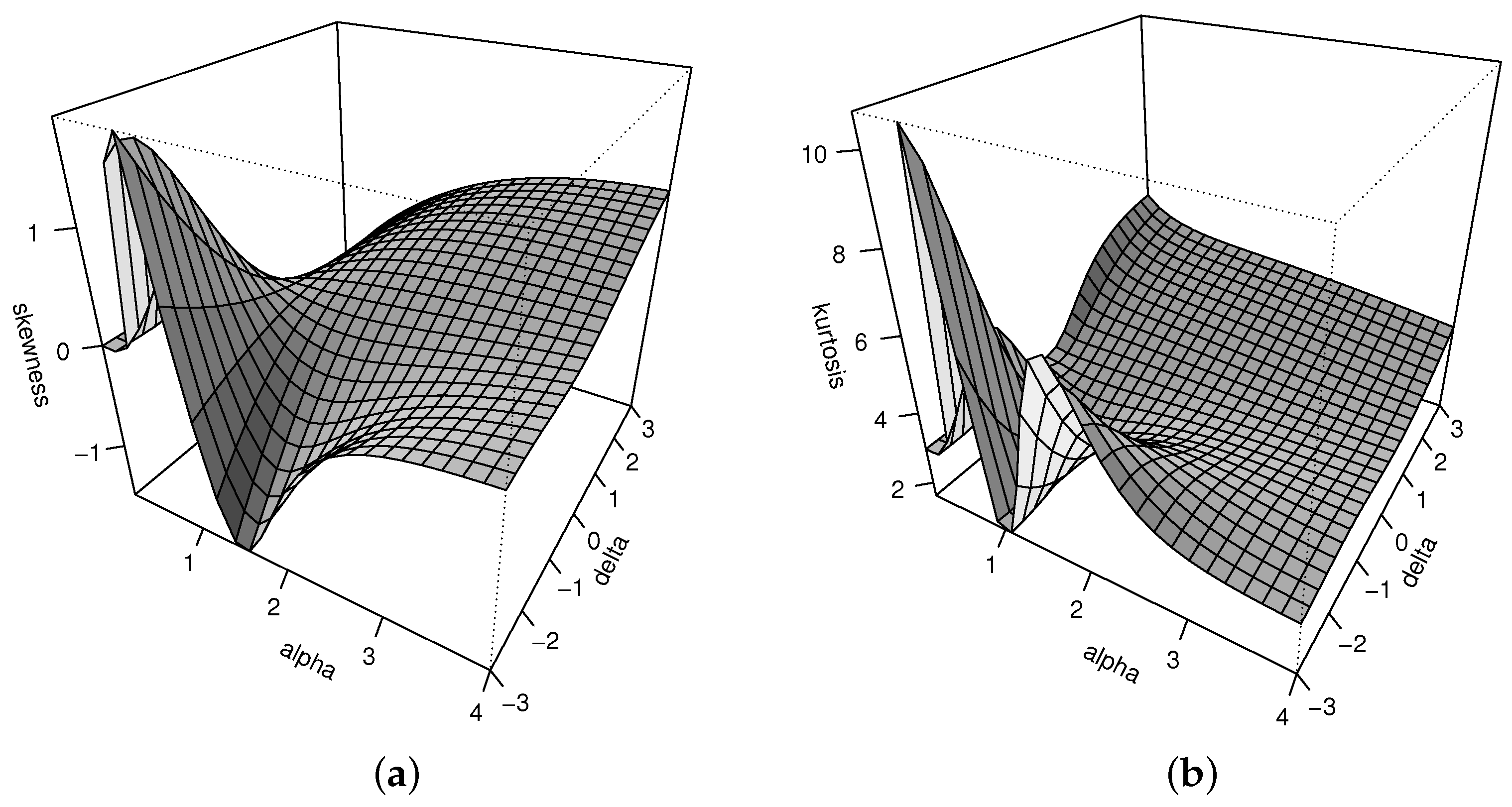
respectively. Figure 2 shows the asymmetry and kurtosis coefficients for the FPN model with different values of and .
2.4. The Location-Scale Extension
We consider now the location-scale extension for the model. The FPN distribution with location parameter and scale parameter is defined as the distribution of the random variable , for which the pdf is given by:
If X has a density function as in the Equation (7) model, we use the notation .
3. Inference for the FPN Model
In this section, we discuss the ML estimation of the parameters of the FPN model. Observed and expected (Fisher) information matrices are derived for the standard and location-scale models. For the location-scale situation, we have a four-dimension parameter vector, .
3.1. Standard Case
Considering that are independent and identically distributed with standard FPN distribution, the log-likelihood function for based on the sample is given by:
from which the elements of the score function are given by:
where
Equating the above derivatives to zero, we obtain the ML equations, which are given by:
To solve the above equations, a numerical procedure is required since analytical solutions are not available. To derive the Fisher information matrix, we consider the second derivatives of the log-likelihood function for parameters , which we denote by (); these are given by:
where
| , | , | |
| , | , | . |
The elements of the Fisher information matrix are obtained by computing the expected values of the corresponding elements of the observed information matrix.
3.2. The Location-Scale Model
For a random sample of size n, , from the distribution, the likelihood function for based on the sample can be written as:
where . The elements of the score function are given by:
where , and sign is the sign function. The solutions for the score equations are given by:
where
3.3. Expected Information Matrix
For an observation () we have that:
where . The second derivatives of the log-likelihood function (11) with respect to the model parameters are given by:
where are defined in Section 3.1. Note that , , and . Denoting as the expected values of the elements of the observed information matrix and defining for , and we obtain:
must be computed numerically since they have no closed forms.
4. Simulating Values from the FPN Model
In this section, we discuss three methods for drawing values from the FPN distribution. This model has no stochastic representation, nor does it have a tractable cdf, making data simulation by conventional methods difficult. On the other hand, as the FPN is a location-scale model, we only discuss the case and .
4.1. Acceptance-Rejection Method: Way 1
This method can be used for . Note that the pdf of the FPN model can be written as
where and is the pdf of the PN. For this reason, to draw values from the standard FPN model, we can use the following algorithm:
- Simulate .
- Simulate .
- Simulate .
- Do .
- If , accept Y. Otherwise, back to step 1.
The probability of a value being accepted is .
4.2. Acceptance-Rejection Method: Way 2
This method can be used for . Note that:
where and is the pdf of the . For this reason, to draw values from the standard FPN model, we can use the following algorithm:
- Simulate .
- Simulate .
- Simulate independently.
- Do .
- If , do . Otherwise, do .
- Do .
- If , accept Y. Otherwise, back to step 1.
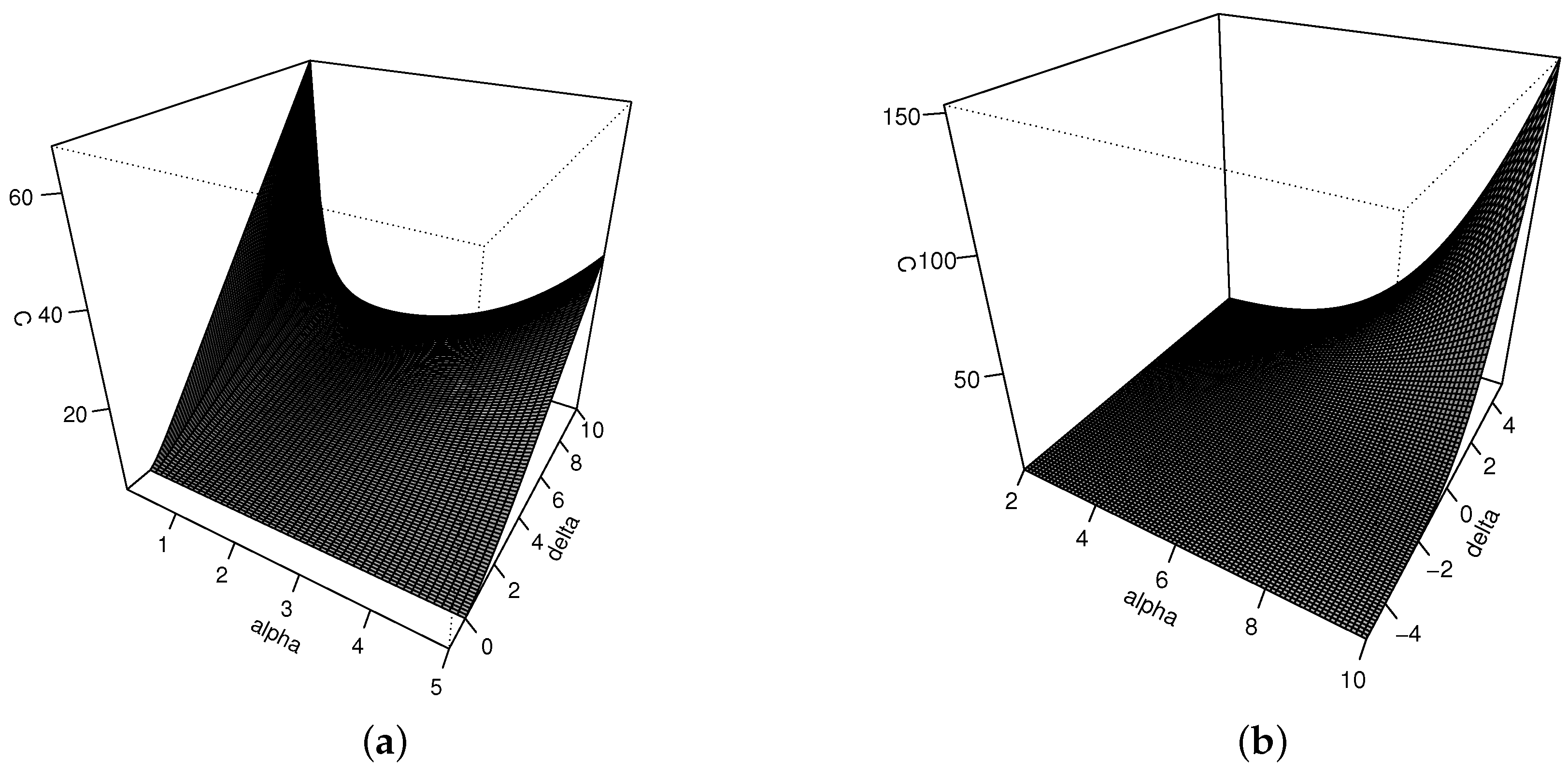
The probability of a value being accepted is . Figure 3 shows the constant C for the two ways discussed of drawing values from the FPN model. Results suggest that neither method is appropriate for drawing values from the FPN model for large values of .
4.3. A Metropolis-Hastings Algorithm
The Metropolis–Hastings algorithm is used extensively in a Bayesian context, because it allows values to be drawn from a given pdf, as long as we know its kernel (and not necessarily a possible normalizing constant). For the FPN distribution, that kernel is given by:
The method requires a proposal distribution, for which we considered the model. The detail of the algorithm is as follows:
- Define an initial value .
- For , draw and . Do .
- Define .
- If , do . Otherwise, .
represent a sample of size n from the FPN distribution. In order to decrease the correlation of the values drawn, we draw values. The first b values are discarded (the burn-in) and for t values we only consider 1 (the thin). In particular, we consider 1000, and , showing a satisfactory performance of the method for all the combinations of and considered in this work.
5. Simulation Studies
In this Section, we present three simulation studies. The first study illustrates the performance of the three simulation procedures in drawing values from the model discussed in Section 4. The second study is devoted to assessing the performance of the ML estimators in finite samples. The third study shows a model selection problem to select among the N, PN and FPN models when the data are generated under different scenarios.
5.1. Assessing the Simulation Procedures for the FPN Model
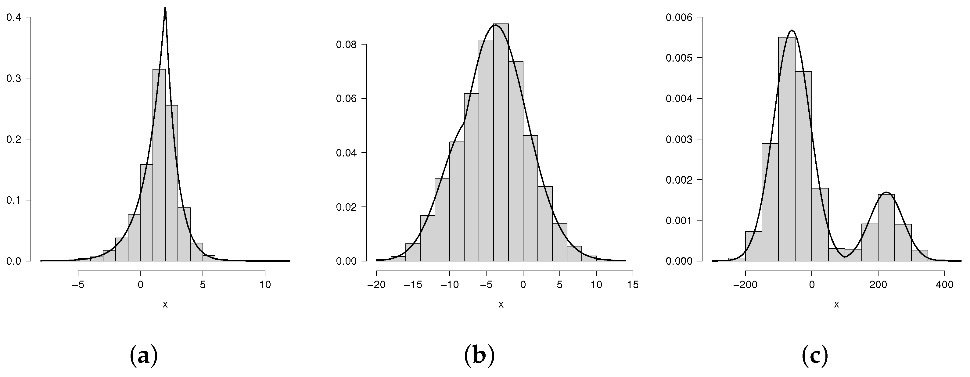
In this Section, we study the three methods discussed in Section 4 to simulate values from the FPN distribution. Figure 4 shows the histogram versus the theoretical curve for 10,000 values drawn from three combinations of parameters for the FPN model, using the three methods discussed previously. Note that, except for restrictions in the acceptance-rejection method given in the two ways (i.e., and for way 1 and way 2, respectively) the three methods seem suitable for drawing values from the model.
On the other hand, we evaluate the execution times of the three ways of drawing values (when the comparison is possible). For this, we draw 100 samples for the FPN model of size 1000; 2000 and 5000 and compute the average of these execution times. We consider , , ranging in and ranging in . The results for the three methods were very similar (with differences lower than 0.01 s). For instance, considering all the combinations for and and 5000 (the case that took the longest), the maximum average of the execution times was 0.9134 s, suggesting that is relatively quick to simulate values from the model in all cases. As the Metropolis-Hastings algorithm can be applied for the FPN model in all situations, this method was used for data generation hereinafter.
5.2. Performance of ML Estimators in Finite Samples
In order to evaluate the properties of ML estimators in finite samples, the samples were generated based on the Metrópolis-Hastings algorithm discussed in the previous section.
In all cases, we consider and as true values. The sample sizes considered were and with three values for (0.5, 1.0 and 1.5) and (−0.5, 0.0 and 0.5). The three values for represent the bimodal asymmetric, bimodal symmetric and unimodal cases respectively, totaling 18 different cases. For each, we drew 1000 replicates and we computed the ML estimators using the optim function in R. We present the mean of the estimates and the mean of the estimated standard errors for the 1000 replicates. Results are presented in Table 1, showing that the mean of the estimates converges to the true value, and the mean of the estimated standard errors is reduced for all the parameters when n is increased, suggesting that the ML estimators for the FPN model are consistent.
5.3. A Model Selection Study
In this Section, we consider a simulation study in order to assess two model selection criteria in different contexts based on the FPN model: the AIC (see Akaike [21]), namely
where is the ML estimator of and k is the number of parameters for the fitted model; and the Bayesian criterion (see Schwarz [22]), defined as
Models with lower AIC and BIC are preferred. The data were drawn from the FPN model, with varying in and varying in . Note that the FPN corresponds to the N distribution and FPN corresponds to the PN model. Again, we consider two sample sizes: 200 and 500. For each simulated sample, we fitted the N, PN and FPN models and selected a model based on AIC and BIC criteria. Table 2 summarizes the percentage of times where each model is chosen based on the two criteria. Note that for and (where the data are drawn from the N model), both criteria effectively chose the N model more frequently than the other models. However, for and (where the data are drawn from the PN model), both criteria continue to choose the N model more frequently (except for the case , and ), suggesting that AIC and BIC criteria choose the N model over the other models in scenarios where the asymmetry and the sample size are greater. For all other cases, we note that the BIC criterion tends to choose the N model—incorrectly—much more frequently than the AIC criterion, and the advantages of the FPN model are evidenced in cases where is increased.
6. Numerical Illustrations
In this Section, we illustrate with two real datasets the better performance of the FPN distribution compared with other models in the literature. Codes were developed in Core Team R [23] and are available as supplementary material for this manuscript.
6.1. Illustration 1
The first dataset corresponds to 481 observations of the variable “Crack” included in the dataset verb “Pollen5.Dat” available at http://lib.stat.cmu.edu/datasets/pollen.data, accessed on 15 October 2021. A descriptive summary of the data can be found in Table 3. Quantities and denote, respectively, the sample asymmetry and kurtosis coefficients.
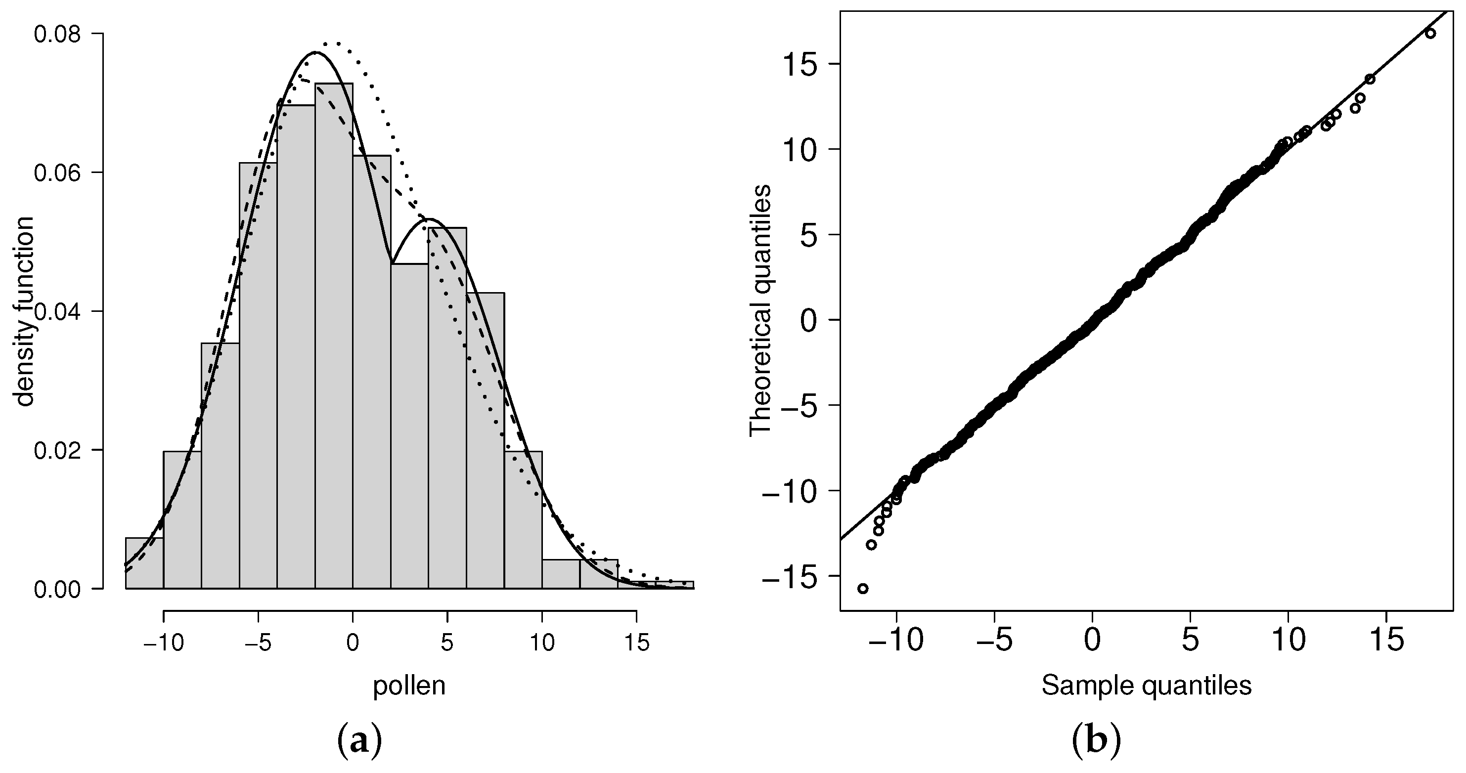
Clearly, the values taken by the asymmetry and kurtosis coefficients indicate that an asymmetric model may be more adequate than a symmetric model for fitting the pollen data. Moreover, the data histogram presented in Figure 5a shows that a model with the ability to fit bimodal data may present better results than just the PN model. To quantify the findings we test the hypothesis
by using the likelihood ratio statistic
leading to
which is greater than the 5% critical value for the chi-square distribution with one degree of freedom, given by Hence, there is a clear indication that the FPN model can be quite useful in fitting bimodal data such as the pollen data described above. Table 4 presents parameter estimates (standard errors in parentheses) for both the FPN and ordinary models, including the mixture of normals (MN). Finally, plots for the fitted PN, MN and FPN models are presented in Figure 5b. Likewise, we present the qq-plot that follows by using parameter estimates for the FPN model, suggesting a good fit of the model for this dataset.
To compare model fit, we consider the AIC and BIC criteria. Hence, we have that the FPN model presents the best fit for the pollen dataset, of all the models considered.
6.2. Illustration 2
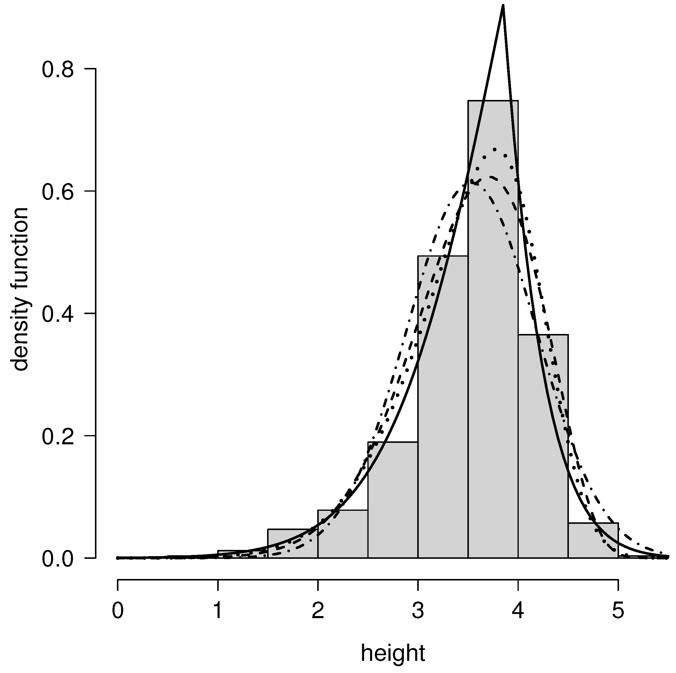
The dataset consists of 1150 heights measured at 1 micron intervals along the drum of a roller (i.e., parallel to the axis of the roller). This was part of an extensive study of surface roughness of the rollers. The units of height are not given, because the data are automatically rescaled as they are recorded, and the scaling factor is imperfectly known. The zero reference height is arbitrary. Data are available for downloading at http://lib.stat.cmu.edu/jasadata/laslett, accessed on 15 October 2021. More details about the data can be found in Laslett [24]. Table 5 shows the summary statistics for the data. Note that the data have a large, negative sample asymmetry and sample kurtosis greater than three, indicating that the ordinary normal model may present a poor fit. Table 6 presents the fit for the N, SN, PN and FPN models. Note that the minimum AIC and BIC criteria are attached by the FPN distribution. Finally, Figure 6 presents the histogram for the data and the fitted pdf for the models, showing the better performance of the FPN distribution over the other models considered.
7. Conclusions
The main object of this paper is to propose a new asymmetric model that is more flexible than the generalized Gaussian model studied in Durrans [2]. This new model includes a parameter that makes it more flexible, because it is useful for unimodal or bimodal data and/or cases with skewness and kurtosis larger than those expected for the N and PN models. Given the flexibility of the model, further work could study the FPN distribution in different contexts: regression, measurement with error-in-variable models, random effect models, and so forth.
Author Contributions
Conceptualization, G.M.-F. and H.W.G.; methodology, H.W.G.; software, D.I.G. and G.M.-F.; validation, G.M.-F., H.W.G. and H.B.; formal analysis, G.M.-F., O.V. and H.W.G.; investigation, H.W.G., O.V. and G.M.-F.; writing—original draft preparation, G.M.-F. and D.I.G.; writing—review and editing, O.V. All authors have read and agreed to the published version of the manuscript.
Funding
Héctor W. Gómez’s research has been partially supported by SEMILLERO UA-2021.
Institutional Review Board Statement
Not applicable.
Informed Consent Statement
Not applicable.
Data Availability Statement
Data are available for downloading at http://lib.stat.cmu.edu/datasets/pollen.data (accessed on 15 October 2021) and http://lib.stat.cmu.edu/jasadata/laslett (accessed on 15 October 2021).
Conflicts of Interest
The authors declare no conflict of interest.
References
- Azzalini, A. A class of distributions which includes the normal ones. Scand. J. Stat. 1985, 12, 171–178. [Google Scholar]
- Durrans, S.R. Distributions of fractional order statistics in hydrology. Water Resour. Res. 1992, 28, 1649–1655. [Google Scholar] [CrossRef]
- McLachlan, G.; Peel, D. Finite Mixture Models; John Wiley & Sons, Inc.: New York, NY, USA, 2000. [Google Scholar]
- Marin, J.; Mengersen, K.; Robert, C.P. Bayesian Modeling and Inference for mixtures of distributions. In Handbook of Statistics; Dey, D., Rao, C., Eds.; Elsevier: Amsterdam, The Netherlands, 2005; pp. 454–508. [Google Scholar]
- Azzalini, A.; Capitanio, A. Distributions generate by perturbation of symmetry with emphasis on a multivariate skew-t distribution. J. R. Stat. Soc. Ser. B 2003, 65, 367–389. [Google Scholar] [CrossRef]
- Ma, Y.; Genton, M.G. Flexible class of skew-symmetric distributions. Scand. J. Stat. 2004, 31, 459–468. [Google Scholar] [CrossRef] [Green Version]
- Arellano-Valle, R.B.; Gómez, H.W.; Quintana, F.A. Statistical inference for a general class of asymmetric distributions. J. Stat. Plan. Inference 2005, 128, 427–443. [Google Scholar] [CrossRef]
- Kim, H.J. On a class of two-piece skew-normal distributions. Statistics 2005, 39, 537–553. [Google Scholar] [CrossRef]
- Lin, T.I.; Lee, J.C.; Hsieh, W.J. Robust mixture models using the skew-t distribution. Stat. Comput. 2007, 17, 81–92. [Google Scholar] [CrossRef]
- Lin, T.I.; Lee, J.C.; Yen, S.Y. Finite mixture modeling using the skew-normal distribution. Stat. Sin. 2007, 17, 909–927. [Google Scholar]
- Elal-Olivero, D.; Gómez, H.W.; Quintana, F.A. Bayesian Modeling using a class of Bimodal skew-Elliptical distributions. J. Stat. Plan. Inference 2009, 139, 1484–1492. [Google Scholar] [CrossRef]
- Arnold, B.C.; Gómez, H.W.; Salinas, H.S. On multiple constraint skewed models. Statistics 2009, 43, 279–293. [Google Scholar] [CrossRef]
- Arnold, B.C.; Gómez, H.W.; Salinas, H.S. A doubly skewed normal distribution. Statistics 2015, 49, 842–858. [Google Scholar] [CrossRef]
- Gómez, H.W.; Elal-Olivero, D.; Salinas, H.S.; Bolfarine, H. Bimodal extension based on the skew-normal distribution with application to pollen data. Environmetrics 2011, 22, 50–62. [Google Scholar] [CrossRef]
- Braga, A.D.S.; Cordeiro, G.M.; Ortega, E.M.M. A new skew-bimodal distribution with applications. Commun. Stat.-Theory Methods 2018, 47, 2950–2968. [Google Scholar] [CrossRef]
- Venegas, O.; Salinas, H.S.; Gallardo, D.I.; Bolfarine, B.; Gómez, H.W. Bimodality based on the generalized skew-normal distribution. J. Stat. Comput. Simul. 2018, 88, 156–181. [Google Scholar] [CrossRef]
- Gómez-Déniz, E.; Pérez-Rodríguez, J.V.; Reyes, J.; Gómez, H.W. A Bimodal Discrete Shifted Poisson Distribution. A Case Study of Tourists’ Length of Stay. Symmetry 2020, 12, 442. [Google Scholar] [CrossRef] [Green Version]
- Lehmann, E.L. The power of rank tests. Ann. Math. Stat. 1953, 24, 23–43. [Google Scholar] [CrossRef]
- Gupta, D.; Gupta, R.C. Analyzing skewed data by power normal model. Test 2008, 17, 197–210. [Google Scholar] [CrossRef]
- Pewsey, A.; Gómez, H.W.; Bolfarine, H. Likelihood-based inference for power distributions. Test 2012, 21, 775–789. [Google Scholar] [CrossRef]
- Akaike, H. A new look at statistical model identification. IEEE Trans. Autom. Control 1974, 19, 716–723. [Google Scholar] [CrossRef]
- Schwarz, G. Estimating the dimension of a model. Ann. Stat. 1978, 1, 461–464. [Google Scholar] [CrossRef]
- Core Team, R. R: A Language and Environment for Statistical Computing; R Foundation for Statistical Computing: Vienna, Austria, 2021. [Google Scholar]
- Laslett, G.M. Kriging and Splines: An Empirical Comparison of Their Predictive Performance in Some Applications: Rejoinder. J. Am. Stat. Assoc. 1994, 89, 406–409. [Google Scholar] [CrossRef]
Figure 1.
Pdf for FPN with different combinations of and : (a) FPN and varying ; (b) FPN and varying ; (c) FPN and varying ; and (d) FPN and varying .
Figure 1.
Pdf for FPN with different combinations of and : (a) FPN and varying ; (b) FPN and varying ; (c) FPN and varying ; and (d) FPN and varying .

Figure 2.
(a) Skewness and (b) kurtosis coefficients for the FPN model.

Figure 3.
Constant C for the acceptance-rejection method to draw values from FPN model: (a) way 1 and (b) way 2.
Figure 3.
Constant C for the acceptance-rejection method to draw values from FPN model: (a) way 1 and (b) way 2.

Figure 4.
Ten thousand values simulated from the FPN model under different scenarios: (a) , and acceptance-rejection method: way 1; (b) and acceptance-rejection method: way 2; (c) and Metropolis-Hastings method.
Figure 4.
Ten thousand values simulated from the FPN model under different scenarios: (a) , and acceptance-rejection method: way 1; (b) and acceptance-rejection method: way 2; (c) and Metropolis-Hastings method.

Figure 5.
(a) Fitted distributions: SN (dotted line), MN (dashed line) and FPN (solid line) models. (b) Simulated QQ-plot for the fitted FPN model and the variable pollen.
Figure 5.
(a) Fitted distributions: SN (dotted line), MN (dashed line) and FPN (solid line) models. (b) Simulated QQ-plot for the fitted FPN model and the variable pollen.

Figure 6.
Histogram of heights dataset and fitted models N (dotted-dashed line), SN (dotted line), PN (dashed line) and FPN (solid line).
Figure 6.
Histogram of heights dataset and fitted models N (dotted-dashed line), SN (dotted line), PN (dashed line) and FPN (solid line).


Table 1.
Mean of the estimates and mean of the estimated standard errors (in parentheses) based on 1000 replicates for the FPN model. In all cases , are maintained and different sample sizes and values for and are considered.
Table 1.
Mean of the estimates and mean of the estimated standard errors (in parentheses) based on 1000 replicates for the FPN model. In all cases , are maintained and different sample sizes and values for and are considered.
| Parameter | |||||||
|---|---|---|---|---|---|---|---|
| 0.4861 (4.4259) | −0.2412 (2.0642) | −0.1071 (1.5502) | −0.0133 (1.2664) | −0.0065 (1.0174) | −0.0029 (0.8505) | ||
| 0.9068 (0.5161) | 0.9280 (0.4248) | 0.9340 (0.3629) | 0.9258 (0.3173) | 0.9382 (0.2802) | 0.9469 (0.2468) | ||
| 0.1195 (0.0990) | 0.1109 (0.0774) | 0.1136 (0.0719) | 0.1101 (0.0637) | 0.1093 (0.0640) | 0.1081 (0.0601) | ||
| −0.8799 (1.3637) | −0.6915 (0.6524) | −0.4955 (0.4797) | −0.3877 (0.3809) | −0.1621 (0.3485) | −0.0117 (0.3129) | ||
| −0.022 (0.134) | 0.000 (0.085) | 0.054 (0.150) | 0.011 (0.124) | 0.000 (0.064) | −0.007 (0.031) | ||
| 0.971 (0.100) | 0.989 (0.065) | 0.923 (0.132) | 0.953 (0.090) | 0.977 (0.189) | 1.009 (0.118) | ||
| 0.835 (0.096) | 0.809 (0.060) | 0.846 (0.150) | 0.870 (0.123) | 0.895 (0.155) | 0.833 (0.079) | ||
| −0.587 (0.225) | −0.532 (0.145) | −0.163 (0.281) | −0.109 (0.181) | 0.450 (0.439) | 0.515 (0.277) | ||
| 0.006 (0.126) | −0.007 (0.081) | 0.018 (0.129) | 0.017 (0.105) | −0.003 (0.069) | −0.013 (0.038) | ||
| 0.965 (0.108) | 0.984 (0.070) | 0.928 (0.135) | 0.947 (0.088) | 0.991 (0.206) | 1.008 (0.126) | ||
| 1.011 (0.112) | 1.009 (0.072) | 1.065 (0.178) | 1.058 (0.138) | 1.184 (0.352) | 1.060 (0.104) | ||
| −0.578 (0.243) | −0.540 (0.156) | −0.167 (0.309) | −0.122 (0.197) | 0.493 (0.516) | 0.510 (0.298) | ||
| −0.003 (0.122) | 0.008 (0.079) | 0.050 (0.112) | −0.016 (0.096) | −0.016 (0.096) | −0.018 (0.03) | ||
| 0.970 (0.115) | 0.983 (0.074) | 0.921 (0.136) | 0.964 (0.092) | 0.963 (0.092) | 1.011 (0.126) | ||
| 1.515 (0.190) | 1.498 (0.115) | 1.479 (0.241) | 1.504 (0.207) | 1.604 (0.207) | 1.501 (0.154) | ||
| −0.584 (0.273) | −0.541 (0.173) | −0.175 (0.343) | −0.104 (0.228) | 0.545 (0.527) | 0.524 (0.330) | ||
Table 2.
Percentage of times where AIC and BIC choose the N, PN and FPN models based on 1000 replicates for different scenarios for the FPN model and sample size.
Table 2.
Percentage of times where AIC and BIC choose the N, PN and FPN models based on 1000 replicates for different scenarios for the FPN model and sample size.
| −1.5 | −0.5 | 0.0 | 0.5 | 2.0 | ||||||||
| Fitted Model | AIC | BIC | AIC | BIC | AIC | BIC | AIC | BIC | AIC | BIC | ||
| 200 | 0.5 | N | 0.0 | 0.2 | 42.0 | 85.4 | 65.2 | 93.6 | 35.0 | 77.9 | 2.6 | 19.5 |
| PN | 2.2 | 6.6 | 8.9 | 3.7 | 25.0 | 6.1 | 16.0 | 9.4 | 0.9 | 1.3 | ||
| FPN | 97.8 | 93.2 | 49.1 | 10.9 | 9.8 | 0.3 | 49.0 | 12.7 | 96.5 | 79.2 | ||
| 0.8 | N | 0.0 | 0.0 | 41.4 | 90.2 | 76.0 | 97.5 | 52.0 | 91.8 | 5.3 | 35.1 | |
| PN | 0.1 | 0.1 | 9.3 | 1.8 | 12.7 | 2.1 | 9.0 | 2.1 | 1.6 | 1.3 | ||
| FPN | 99.9 | 99.9 | 49.3 | 8.0 | 11.3 | 0.4 | 39.0 | 6.1 | 93.1 | 63.6 | ||
| 1.0 | N | 0.0 | 0.0 | 48.2 | 92.4 | 76.3 | 97.7 | 53.1 | 92.0 | 6.0 | 38.4 | |
| PN | 0.0 | 0.0 | 10.9 | 3.1 | 12.9 | 1.9 | 10.2 | 2.9 | 2.3 | 2.6 | ||
| FPN | 100.0 | 100.0 | 40.9 | 4.5 | 10.8 | 0.4 | 36.7 | 5.1 | 91.7 | 59.0 | ||
| 1.5 | N | 0.0 | 1.4 | 63.1 | 96.8 | 71.6 | 94.8 | 43.2 | 82.3 | 5.7 | 35.5 | |
| PN | 4.1 | 9.9 | 11.5 | 2.1 | 16.7 | 4.8 | 25.7 | 12.3 | 6.1 | 9.3 | ||
| FPN | 95.9 | 88.7 | 25.4 | 1.1 | 11.7 | 0.4 | 31.1 | 5.4 | 88.2 | 55.2 | ||
| 3.0 | N | 50.1 | 88.0 | 71.3 | 94.0 | 49.6 | 83.3 | 26.6 | 63.6 | 1.7 | 13.2 | |
| PN | 19.3 | 11.1 | 20.5 | 6.0 | 37.7 | 15.6 | 48.2 | 33.8 | 25.7 | 48.7 | ||
| FPN | 30.6 | 0.9 | 8.2 | 0.0 | 12.7 | 1.1 | 25.2 | 2.6 | 72.6 | 38.1 | ||
| 500 | 0.5 | N | 0.0 | 0.0 | 11.8 | 69.2 | 47.9 | 87.2 | 10.7 | 52.8 | 0.1 | 0.4 |
| PN | 0.1 | 0.4 | 4.2 | 1.8 | 39.0 | 12.1 | 9.8 | 11.2 | 0.0 | 0.0 | ||
| FPN | 99.9 | 99.6 | 84.0 | 29.0 | 13.1 | 0.7 | 79.5 | 36.0 | 99.9 | 99.6 | ||
| 0.8 | N | 0.0 | 0.0 | 13.6 | 76.3 | 72.2 | 97.6 | 25.6 | 82.6 | 0.0 | 1.4 | |
| PN | 0.0 | 0.0 | 3.9 | 1.1 | 16.1 | 2.3 | 3.5 | 1.8 | 0.0 | 0.0 | ||
| FPN | 100.0 | 100.0 | 82.5 | 22.6 | 11.7 | 0.1 | 70.9 | 15.6 | 100.0 | 98.6 | ||
| 1.0 | N | 0.0 | 0.0 | 17.4 | 80.8 | 77.4 | 98.4 | 25.4 | 84.0 | 0.0 | 2.2 | |
| PN | 0.0 | 0.0 | 5.7 | 1.7 | 13.7 | 1.6 | 4.6 | 1.9 | 0.0 | 0.0 | ||
| FPN | 100.0 | 100.0 | 76.9 | 17.5 | 8.9 | 0.0 | 70.0 | 14.1 | 100.0 | 97.8 | ||
| 1.5 | N | 0.0 | 0.0 | 41.3 | 95.2 | 60.6 | 94.1 | 15.7 | 68.5 | 0.0 | 2.1 | |
| PN | 0.0 | 0.3 | 10.8 | 2.3 | 29.0 | 5.6 | 26.0 | 19.3 | 0.9 | 2.0 | ||
| FPN | 100.0 | 99.7 | 47.9 | 2.5 | 10.4 | 0.3 | 58.3 | 12.2 | 99.1 | 95.9 | ||
| 3.0 | N | 27.6 | 91.3 | 53.1 | 93.5 | 18.3 | 61.1 | 3.1 | 25.5 | 0.0 | 0.3 | |
| PN | 4.4 | 1.0 | 27.5 | 6.4 | 66.6 | 38.5 | 57.0 | 70.9 | 8.7 | 25.8 | ||
| FPN | 68.0 | 7.7 | 19.4 | 0.1 | 15.1 | 0.4 | 39.9 | 3.6 | 91.3 | 73.9 | ||
Table 3.
Summary statistics for precipitation data.
| n | Mean | Variance | ||
|---|---|---|---|---|
| 481 | −0.0483 | 26.9980 | 0.2329 | 2.5944 |
Table 4.
Parameter estimates (standard errors in parentheses) for N, SN, PN, MN and FPN models in the pollen dataset.
Table 4.
Parameter estimates (standard errors in parentheses) for N, SN, PN, MN and FPN models in the pollen dataset.
| Parameter | N | SN | PN | FPN | Parameter | MN |
|---|---|---|---|---|---|---|
| −0.0489 (0.2367) | −4.9482 (0.8164) | −11.8216 (7.2910) | −2.0300 (0.2797) | −3.5847 (0.8948) | ||
| 5.1902 (0.1673) | 7.1379 (0.6058) | 8.4627 (1.8070) | 3.5192 (0.1982) | 3.3009 (0.3662) | ||
| - | 1.6568 (0.4856) | 7.5132 (7.9838) | 0.7316 (0.0464) | 3.8531 (1.5545) | ||
| - | - | - | −0.6946 (0.1316) | 3.9516 (0.6768) | ||
| - | - | - | - | - | p | 0.5245 (0.1593) |
| Log-likelihood | −1474.64 | −1472.08 | −1472.24 | −1466.33 | −1466.30 | |
| AIC | 2953.28 | 2950.16 | 2950.47 | 2940.66 | 2942.60 | |
| BIC | 2961.63 | 2962.68 | 2963.00 | 2957.36 | 2963.48 |
Table 5.
Summary statistics for roller data.
| n | Mean | Variance | ||
|---|---|---|---|---|
| 1150 | 3.535 | 0.422 | −0.986 | 4.855 |
Table 6.
Parameter estimates (standard errors in parentheses) for N, SN, PN and FPN models in roller dataset.
Table 6.
Parameter estimates (standard errors in parentheses) for N, SN, PN and FPN models in roller dataset.
| Parameter | N | SN | PN | FPN |
|---|---|---|---|---|
| 3.5347 (0.0192) | 4.2475 (0.0284) | 4.5494 (0.0570) | 3.8529 (0.0106) | |
| 0.6497 (0.0135) | 0.9644 (0.0304) | 0.1983 (0.0279) | 0.7589 (0.0634) | |
| - | −2.7578 (0.2529) | 0.0479 (0.0155) | 0.2082 (0.0568) | |
| - | - | - | 1.3045 (0.2064) | |
| Log-likelihood | −1135.87 | −1071.35 | −1085.24 | −1065.92 |
| AIC | 2275.73 | 2148.69 | 2176.84 | 2139.84 |
| BIC | 2285.83 | 2163.84 | 2191.98 | 2160.03 |
Publisher’s Note: MDPI stays neutral with regard to jurisdictional claims in published maps and institutional affiliations. |
© 2021 by the authors. Licensee MDPI, Basel, Switzerland. This article is an open access article distributed under the terms and conditions of the Creative Commons Attribution (CC BY) license (https://creativecommons.org/licenses/by/4.0/).
Share and Cite
MDPI and ACS Style
Martínez-Flórez, G.; Gallardo, D.I.; Venegas, O.; Bolfarine, H.; Gómez, H.W. Flexible Power-Normal Models with Applications. Mathematics 2021, 9, 3183. https://doi.org/10.3390/math9243183
AMA Style
Martínez-Flórez G, Gallardo DI, Venegas O, Bolfarine H, Gómez HW. Flexible Power-Normal Models with Applications. Mathematics. 2021; 9(24):3183. https://doi.org/10.3390/math9243183
Chicago/Turabian StyleMartínez-Flórez, Guillermo, Diego I. Gallardo, Osvaldo Venegas, Heleno Bolfarine, and Héctor W. Gómez. 2021. "Flexible Power-Normal Models with Applications" Mathematics 9, no. 24: 3183. https://doi.org/10.3390/math9243183
Note that from the first issue of 2016, this journal uses article numbers instead of page numbers. See further details here.