
Numerical and Experimental Evaluation of Thermal Conductivity: An Application to Al-Sn Alloys


Department of Mechanical Engineering, Politecnico di Milano, Via La Masa 1, 20156 Milan, Italy
*
Author to whom correspondence should be addressed.
Metals 2021, 11(4), 650; https://doi.org/10.3390/met11040650
Submission received: 31 March 2021
/
Revised: 8 April 2021
/
Accepted: 14 April 2021
/
Published: 16 April 2021
Abstract
:Evaluation of thermal conductivity of composite materials is extremely important to control material performance and stability in thermal applications as well as to study transport phenomena. In this paper, numerical simulation of effective thermal conductivity of Al-Sn miscibility gap alloys is validated with experimental results. Lattice Monte-Carlo (LMC) method is applied to two-phase and three-phase materials, allowing to estimate effective thermal conductivity from micrographs and individual phase properties. Numerical results are compared with literature data for cast Al-Sn alloys for the two-phase model and with a specifically produced powder metallurgy Al-10vol%Sn, tested using laser flash analysis, for a three-phase simulation. A good agreement between numerical and experimental data was observed. Moreover, LMC simulations confirmed the effect of phase morphology as well as actual phase composition on thermal conductivity of composite materials.
1. Introduction
Thermal conductivity is one of the main properties of materials. It describes the heat transfer in solids related to the transmission of vibrational energy from one particle to an adjacent one without motion of material [1]. The evaluation of this property is fundamental to control material performance and stability, as well as to study further transport phenomena, like electrical conductivity [2].
When composite materials are considered, the evaluation of the overall thermal conductivity as a homogeneous property of the material, known as the effective thermal conductivity (λeff), can become a little tricky. Equilibrium properties of composites, like density and heat capacity, can be determined as a weighted average of constituents’ properties with respect to volume or mass. On the other hand, morphology must be taken into account as well for transport properties like thermal conductivity [3]. In more detail, this means that distribution, shape, and orientation of phases must be considered in addition to thermal conductivity of each phase and its volume fraction.
From a computational point of view, various analytical equations have been developed for particular structures, such as Maxwell-Eucken, Bruggeman, and Progelhof models [4,5]. The limit of this kind of model is that they consider an idealized microstructure and not the real morphology of the material, such as when assuming one phase as inclusion in a matrix with a spherical or cylindrical shape. Therefore, for real multiphase composites with a more complex morphology, it is necessary to use numerical simulations, like direct simulation with finite elements [6,7,8] or Lattice Monte Carlo (LMC) simulation [4,9,10]. The LMC method can statistically predict the effective thermal conductivity (λeff) of a two-dimension or three-dimension multiphase material, considering the random walk of energy particles in a lattice model describing its phase volume fraction, distribution, and size. The starting point for the application of this method can be a micrograph (2D) or a tomography (3D) [4,11]. Each node of the lattice derived from images, arranged in a simple cubic structure, has the properties of the local material. In this way, any geometry of interest can be represented such as starting from a micrograph [12]. In LMC methods applied to the estimation of a multiphase material, a fundamental role is played by the jump probability [9]. The jump probability of a particle to one of the surrounding nodes is a function of thermal conductivity of the phases. The effective thermal conductivity is related to the probability that N jump attempts are successful or unsuccessful in a time interval t. This probability depends on thermal conductivities of original and destination nodes and it is described by the particle displacement vector R. This relation is described by Equation (1).
where λmax is the maximum thermal conductivity of all phases, <R2> is the mean square displacement of all energy particles, and N is the number of jump attempts. Therefore, λeff is the average effective thermal conductivity. In addition, λeff can be estimated along directional components of R. Further details about the equations used in the LMC method are presented in a dedicated paper by Li and Gariboldi [13].
λeff = <R2> * λmax/N
The main challenge in the application of the LMC method is how to obtain meaningful results in a reasonable computational time. In more detail, two aspects are fundamental: the image magnification must be appropriate to show clearly the overall distribution of phases and the lattice model must effectively describe the microstructural features without being too fine, causing a long computational time. The LMC method has, thus, a huge potential in simulating a thermal response of composite materials, taking into account the real microstructural features that cannot be represented in analytical methods.
From an experimental point of view, many techniques are available for characterizing thermal conductivity. The choice of the appropriate method depends on the material class (metallic, polymeric, ceramic), their melting temperature, their expected conductivity/diffusivity, and, in the case of composite materials, their scale length [14]. The latter factor implies that the specimen size for the specific test must allow us to consider the composite material as homogeneous. Therefore, for example, laser flash analysis (LFA, [15,16]) can be applied to a composite material with a sub-millimetric phase size, while a non-conventional experimental setup, like the one proposed by Gariboldi et al. in [14], must be designed according to the specific material structure.
Al-Sn alloys are considered to be the case study to compare numerical and experimental results for effective thermal conductivity. Al-Sn binary alloys are miscibility gap alloys, i.e., they consist of two (almost) completely immiscible phases. Therefore, this system can be considered as a metallic composite material made of two phases: the Al high-melting phase and the Sn low-melting soft phase. Al-Sn alloys are usually applied as bearing materials for their good tribological and mechanical properties [17]. Additionally, they have been proposed as potential alternative anode materials for lithium anode batteries and as anodic corrosion-protective coatings for steels, so it is useful to evaluate transport phenomena and electrical conductivity in particular [2]. Moreover, Sugo et al. [18] suggested applying Al-Sn alloys as metallic phase change materials (PCMs) for thermal energy storage and management. The basic principle behind PCMs is storing the latent heat during a phase transition and releasing it when the transition is reversed. In Al-Sn system, Sn is the phase undergoing the solid-liquid transition, while Al acts as matrix providing mechanical properties and enhancing thermal conductivity. Clearly, in addition to transition temperature and latent heat, thermal conductivity is particularly important in thermal management applications, controlling the rate at which heat is stored or released. The fine microstructure that can be obtained for Al-Sn alloys allows us to consider a relatively small sample that is homogeneous enough to represent the whole material [19]. Therefore, conventional thermal conductivity tests, like LFA, can be applied to characterize these materials.
In the present paper, the LMC numerical method for the analysis of two-phase and three-phase materials is applied to determine thermal conductivity of Al-Sn alloys and results are compared with experimental data. A software for LMC thermal analysis of two-phase materials is validated using experimental data from literature, in which Al-Sn alloys are produced through a cast process. The validation of the version for three-phase materials, where the third phase consists of pores, is conducted on a powder metallurgy Al-Sn sample produced and characterized by the authors.
2. Materials and Methods
2.1. Numerical Method: Lattice Monte-Carlo
A C code was developed by Li and Gariboldi [13] in order to apply the LMC method to 2D micrographs with 2 or 3 phases. The first step is the preparation of representative micrographs describing the material microstructure. Proper single or multiple thresholds must be applied to multi-color or grayscale micrographs, to get a single homogeneous color for each phase. For example, micrographs of two-phase materials are converted in binary images, which have black and white regions only. For this step, two MATLAB scripts were developed for two-phase and three-phase materials, respectively. In this way, the LMC code will be able to distinguish between the phases and it will assign them the corresponding properties, which are the values of thermal conductivity.
Then, the microstructure is mapped into a square lattice model with lattice length L, i.e., L grid nodes along the side of the square area. The number of random particles Num, that will “try to move” in the lattice as well as the number of jump attempts N are set as parameters. As previously said, the jump probability depends on the thermal conductivity of the phase. In more detail, if origin and destination point are in the same phase, the probability is equal to the ratio between the thermal conductivity of the phase normalized with respect to the maximum thermal conductivity of phases, which, in the present case, is thermal conductivity of Al [13]. If the jump is between two different phases (A and B), jump probability at the interface (pAB) is calculated using Equation (2), according to Reference [13].
where λAl and λSn are the thermal conductivities of Al and Sn, respectively. The number of particles Num is usually chosen to be equal to the total number of lattice nodes. The number of jump attempts N is suggested be equal to 105 when L < 100 and to 106 for larger L [13]. The simulation is repeated for a set number of cycles, at least 3, to have statistically representative results. A study on the effect of the different parameters was presented in Reference [13].
2.2. Validation for 2-Phase Materials
The validation of the developed LMC code for two-phase materials was conducted by applying the method to an experimental study by Meydaneri Tezel et al. [20] who reported the experimental characterization of Al-Sn alloys. This study was suitable for the purposes of the present paper, since it presented experimental values of thermal conductivity as well as scanning electron microscopy (SEM, LEO 440, Leica, Wetzlar, Germany) micrographs for various compositions of the Al-Sn binary alloy. Samples, with Al mass content equal to 0%, 0.5%, 2.2%, 25%, 50%, 75%, and 100%, were produced through a casting process involving directional solidification after stirring the molten blend [20]. This method allowed us to obtain flawless and homogeneous samples [20]. Therefore, it is possible to consider them as perfectly binary alloys, where only Al and Sn regions are seen. Based on this assumption, the volume fractions of phases have been calculated here from the given actual composition of the Al alloys, considering their room-temperature densities: 7.31 and 2.70 g/cm3 for Sn and Al, respectively. Thermal conductivity was measured using a radial heat flow apparatus as a function of temperature [20].
Analysis and preparation of SEM micrographs on transversal sections from Reference [20] for an LMC calculation was carried out using ImageJ software (Fiji distribution) [21]. The results of the 2D-LMC calculations will, thus, be related to thermal conductivity in directions perpendicular to the longitudinal axis of the cylindrical sample mentioned in Reference [20] (diameter 30 mm and height 12 mm) in the direction taken into account by the radial heat flow apparatus.
Three areas with lattice length L equal to 150 nodes, i.e., 150 pixels, were chosen for each micrograph of Al-Sn containing 2.2%, 25%, 50%, or 75% in mass of Al, corresponding to about 94.3%, 52.8%, 27.2% and 11.1% in volume of Sn. The corresponding size is 186 µm (41.63 µm for 2.2% Al for which a different magnification had been adopted for a literature micrograph). The Sn-0.5%Al in mass was not considered since it is not possible to clearly distinguish between the two phases. The particle number Num and the number of jumps attempts were set to 22,500, i.e., equal to the number of nodes, and 10,000, respectively. LMC simulations were repeated five times to get statistically representative results. Thermal conductivity at 340 K, 400 K, and 460 K was determined. Thermal conductivity values for the two phases at different temperatures were inferred from the plot of experimental data provided in Reference [20]. The values are reported in Table 1.
Furthermore, a numerical evaluation of λeff was repeated through a direct simulation (DS) with finite elements on the same micrographs at the three reference temperatures. In this steady analysis, λeff can be derived using Equation (3).
where, ΔT is the temperature difference between the two surfaces perpendicular to the considered direction set to 1 K, L is the distance between the two surfaces, and Q is the heat flux. Detailed description of the method was reported in Reference [22].
2.3. Validation for Three-Phase Material
LMC method for three-phase materials was applied to an Al-Sn alloy containing a non-negligible amount of porosity. The main difference with respect to the alloys presented in the previous paragraph is the production process, which can lead more easily to the occurrence of pores.
This Al-Sn based alloy with 10% of Sn in volume was produced through a powder metallurgy process, consisting of powder mixing, compression, and sintering, following a procedure developed in previous studies by the authors [23]. A high purity (>99.7 mass%) atomized Al powder (ECKA Granules GmbH, Fürth, Germany), with particle diameters <45 µm, was simply mixed to Sn powder (Thermo Fisher (Kandel) GmbH-Alfa Aesar, Karlsruhe, Germany) characterized by purity of 99.85% and particle size below 150 µm (100 mesh). The nominal composition of 10% Sn volume corresponds to 23% in mass. Powders were mixed at room temperature in a tumbler mixer (Girafusti Adler T0, Barasso, Italy) for 1 h at 20 rpm. The powder blend was compressed at room temperature using an Instron (Norwood, MA, USA) 1195 100 kN Universal Testing Machine equipped with an extrusion set consisting of a hollow cylinder steel die and a 15-mm-diameter punch. Compression was divided in three steps: loading up to 20 kN with a punch speed of 3 mm/s, then loading up to 53 kN at 1 mm/s, and keeping the maximum load for 1 minute. The resulting specimen is a cylinder with 15 mm in diameter and 15 mm or 8 mm in height. Finally, specimens were sintered at 500 °C for 1 h, in Ar atmosphere to avoid oxidation.
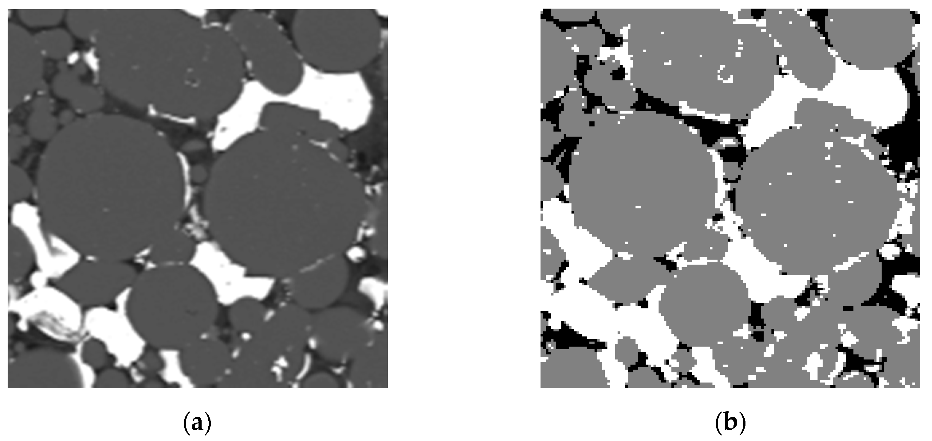
The tallest specimen was cut along a plane parallel to the compression direction for metallographic analysis using Scanning Electron Microscopy (SEM, Sigma 500, Zeiss, Jena Germany). Thanks to the difference in atomic mass between the two elements, chemical etching was not necessary to highlight the phases. The lightest regions consist of Sn, while the darkest ones are pores and the intermediate, dark grey regions correspond to Al. The obtained micrographs were then processed with a MATLAB code to be used for LMC calculation. In this case, two thresholds were applied to obtain three homogeneous regions: Sn (white), Al (grey), and pores (black). An example is given in Figure 1, in a region containing a relatively high amount and irregularly distributed pores.
The shortest specimen was cut along a plane perpendicular to compression direction to obtain a thin sample for LFA. The resulting disk was further cut in a square shape with a side of 10 mm to fit the LFA graphite sample holder. Both top and bottom surfaces were ground with abrasive paper and then covered with a thin graphite layer. The final sample thickness was 1.12 mm. LFA at room temperature was conducted using a Linseis (Selb, Germany) LFA 1000/1600 machine in vacuum. The diffusivity measurement was repeated three times. Thermal conductivity was derived by thermal diffusivity data by multiplying them by specific heat capacity (Cp) and density (ρ). Specific heat capacity for Al-10vol%Sn was determined with thermodynamic calculations as the derivative of enthalpy with respect to temperature at a constant pressure. These calculations were done using Thermo-Calc Software (Version 2020b with TCAL5.1 Al-Alloys Database, Thermo-Calc Software, Stockholm, Sweden) [24]. Density was either calculated with Thermo-Calc Software and measured experimentally using Archimedes’ method (Analytical Balance ME204 with Density Kit Standard and Advanced, Mettler Toledo, Greifensee, Switzerland). The experimental error for thermal conductivity (ελ) is calculated from the relative errors on density (ρ) and thermal diffusivity (α) (Equation (4), [25]).
where δρ and δα are the standard deviations of density and thermal diffusivity obtained experimentally, while , and are the average values of experimental thermal conductivity, density, and thermal diffusivity, respectively.
Three-phase LMC method was applied on 10 areas chosen randomly on a SEM micrograph of diametral section of the sample. Thus, the longitudinal direction of the sample, corresponding to the compression direction, was also the direction for heat propagation in the LFA test. The selected lattice length L was 149 nodes, i.e., 149 pixels, corresponding to 80.54 µm. This number of areas with a relatively small dimension was used to have a reasonable computational time for each simulation, but, at the same time, to have a good statistic supporting the results. To evaluate the effect of the number of particles, two simulation sets were conducted, one with 22,201 particles, corresponding to the number of nodes, and one with 10,000 particles. Less particles can speed up the simulation, but make the result less reliable. Therefore, the number of simulation repetitions was increased from 3 for 22,201 particles to 5 for 10,000 particles. In both cases, the number of jump attempts was set to 10,000. Thermal conductivity of phases at 293 K (20 °C) was set as 63.9 W/(m·K) for Sn [26] and 246.7 W/(m·K) for Al [27]. Considering the sample production process, gas in pores is air, and its thermal conductivity can be approximated to zero (it is 0.0257 W/(m·K) in Reference [28]).
3. Results
3.1. Application of Two-Phases LMC Method
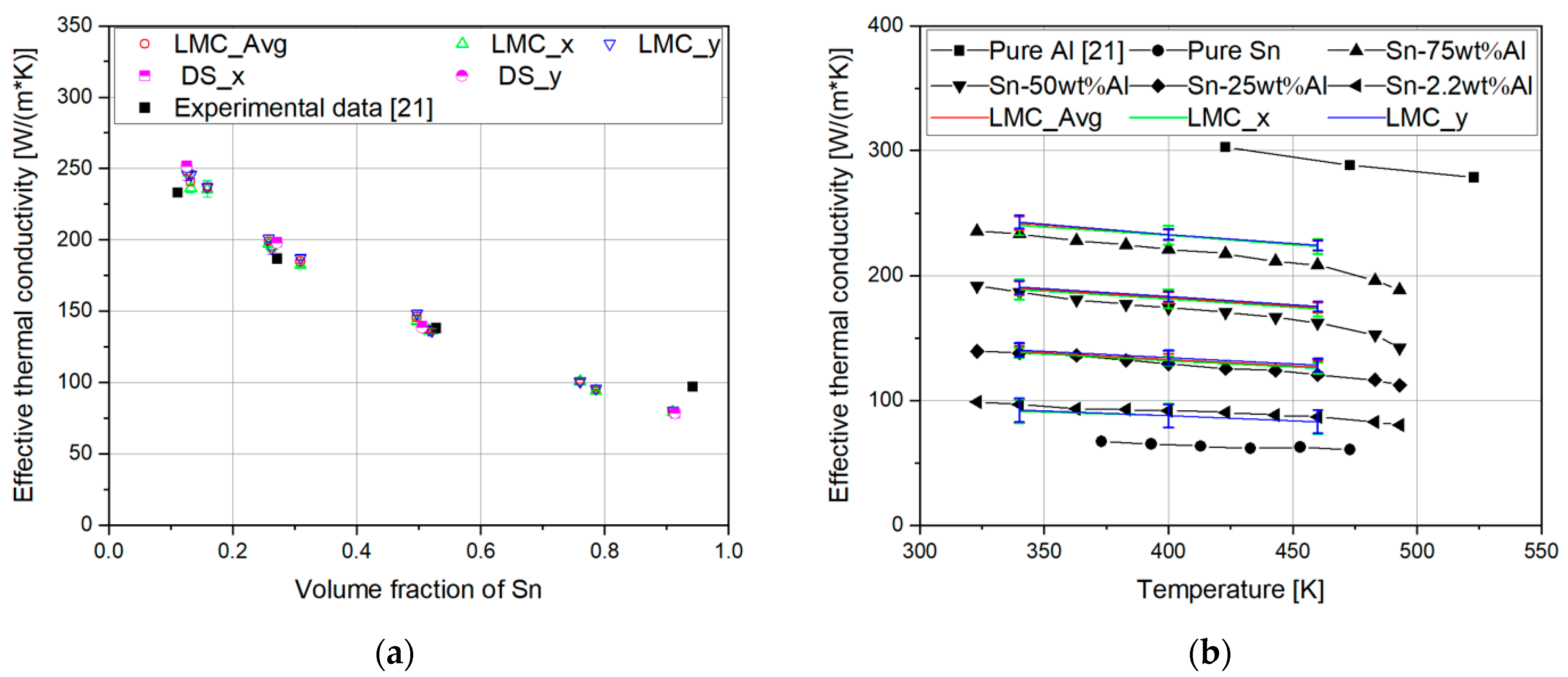
The results of LMC simulation on two-phase Al-Sn alloys are shown in Figure 2 as well as the corresponding experimental results and DS numerical results. Specifically, Figure 2a plots the literature thermal conductivity data [20] at 340 K in terms of their calculated volume fraction of Sn. These data are compared with LMC calculations made for three square regions sampled from the micrograph supplied by Reference [20] for each alloy composition. The results for LMC runs are given both by considering their average thermal conductivity and that, along the horizontal (x) and vertical (y) direction of the square regions, sampled for LMC analyses. Negligible differences can be observed in Figure 2a for thermal conductivity between the x and y directions. Thus, in the following, the only average thermal conductivity has been considered. For LMC calculations of thermal conductivity, the bars plotted in Figure 2a also visualize the difference between maximum and minimum values, which is about ±5 W/(K⋅m) for all the sampled regions. On the other hand, the values for the three regions considered for LMC calculations for the same alloy, clearly show the effect of the actual volume fraction of Sn as well as its variability when these areas are selected from small regions of metallographic samples. For example, for the Sn-50mass%Al, the volume fraction of Sn calculated from chemical composition in Reference [20] is 27.2%and the volume fractions for the three regions used for LMC calculations are very close to it. For the Sn-2.2%Al alloy, the volume % of Sn derived from the chemical composition is 94.3%, while all the three sampled regions displayed lower Sn volume fractions (the average volume of Sn from the micrograph is closer to that derived from the corresponding micrograph in Reference [20]).
Numerical and experimental values of effective thermal conductivity λeff plotted vs. temperature in Figure 2b show a decreasing trend with temperature. At low temperature, the agreement between experimental and calculated data for the same nominal composition are good. The data calculated at a higher temperature are not able to describe the downward curvature displayed by the thermal conductivity of Al-Sn. The downward curvature of high-temperature data from Reference [20] is not displayed by pure Al and Sn.
3.2. Application of Three-Phase LMC Method
3.2.1. Experimental Characterization of Al-10Sn
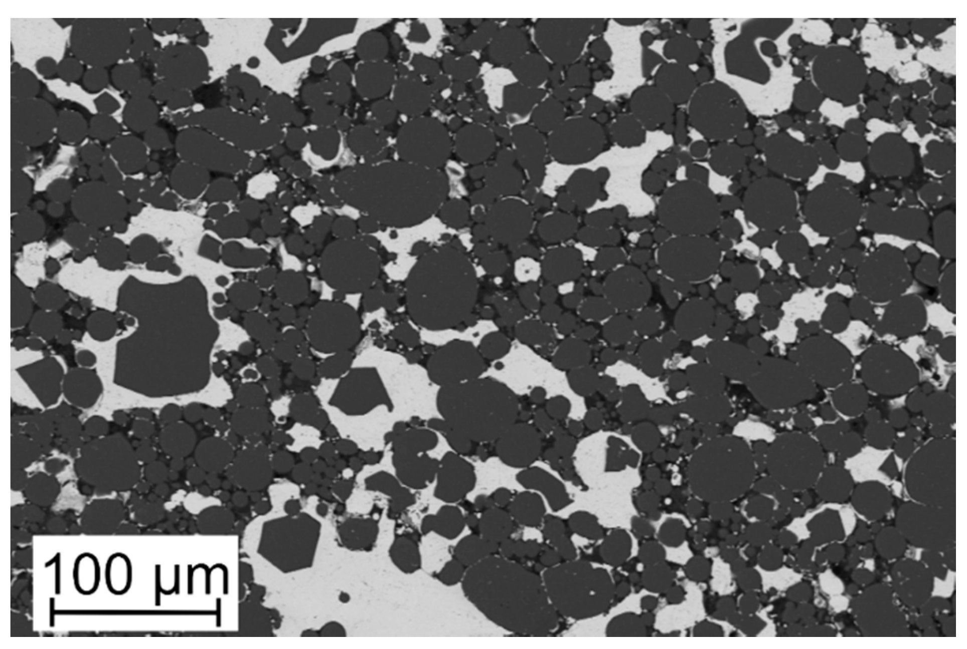
Microstructure of Al-10vol%Sn alloy obtained through powder metallurgy is shown in Figure 3. Light areas correspond to Sn, dark areas correspond to Al, and black areas are pores.
Even after compression, most Al particles have a very circular section. On the other hand, during sintering at 500 °C, Sn melts (melting temperature 232 °C) and it can flow between Al particles. Nevertheless, in the presented sample, the Sn phase is generally located in isolated particles, without forming an interconnected network. Pores can be observed at phase boundaries. According to metallographic analysis on SEM images, porosity volume content is around 8%.
Experimental room-temperature thermal diffusivity data are presented in Table 2 together with other experimental data or thermodynamical properties used to calculate the thermal conductivity. Thermodynamic calculations resulted in a specific heat capacity equal to 0.743 J/(g·K) and theoretical density of 3.16 g/cm3. Experimental density, measured with Archimedes’ method, is 2.90 g/cm3, corresponding to 91.84% of the theoretical value. This result is consistent with porosity measured with metallographic analysis. The average thermal diffusivity measured with LFA is 0.357 cm2/s with a standard deviation of 0.002 cm2/s, i.e., 0.4%. The resulting thermal conductivity is 76.863 ± 0.352 W/(m·K).
3.2.2. LMC Calculation
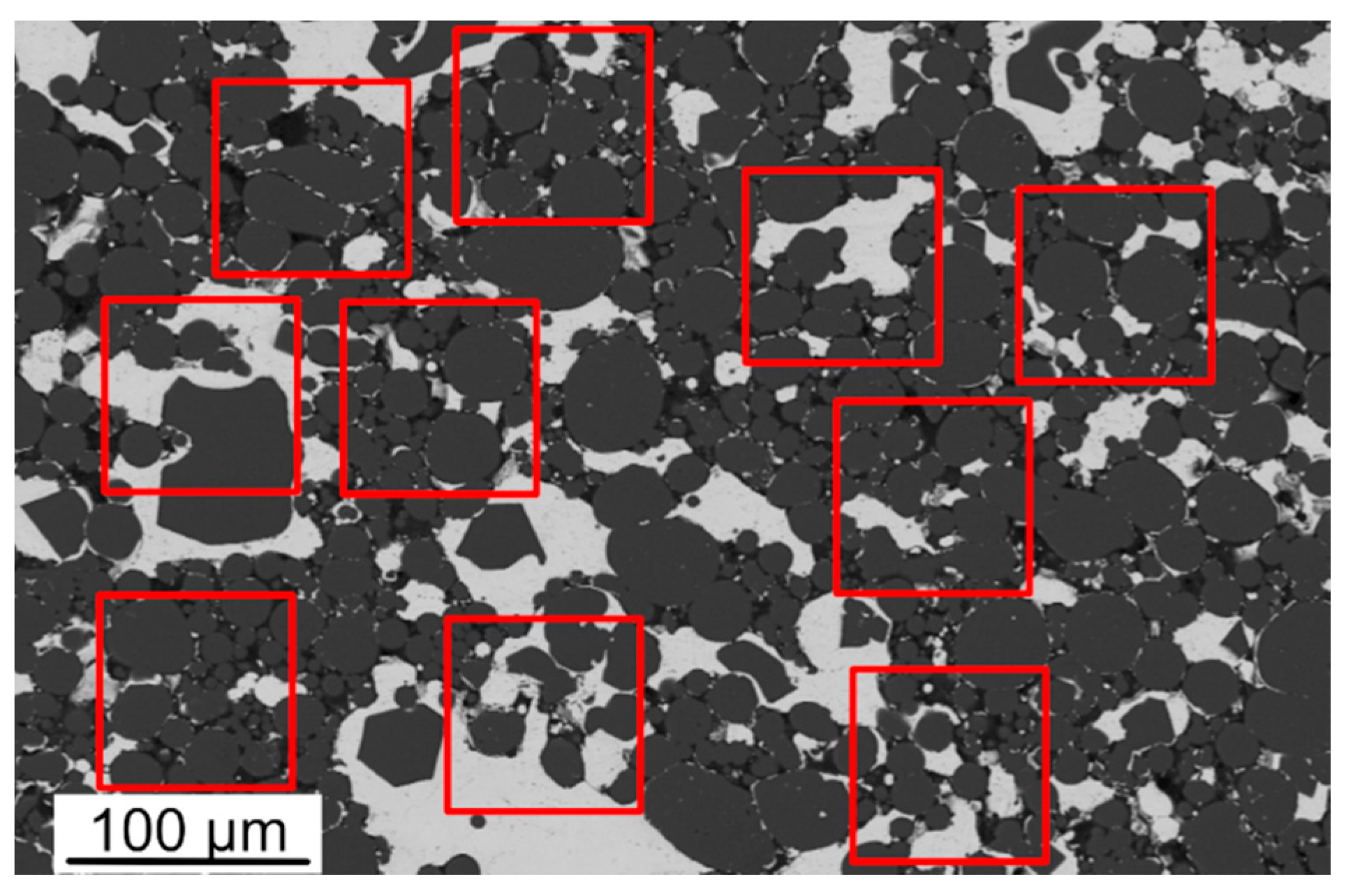
The 10 areas chosen on the SEM micrographs for LMC simulations are shown in Figure 4.
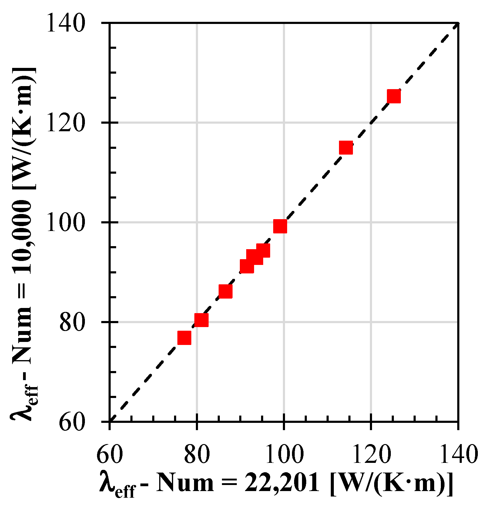
Values of λeff obtained with two different numbers of particles (Num) are compared plotting the series of values with Num = 22,201 on the x-axis and the one with Num = 10,000 on the y-axis in Figure 5. Datapoints are on the bisector of the first quadrant (y = x), which means that the two different parameters for the number of particles result in a close value. The difference is in the standard deviation for the same area after a simulation repetition, which is higher for Num = 10,000 (average value of 0.96 W/(K·m)) than for Num = 22,201 (average value of 0.52 W/(K·m)). In both cases, the standard deviation is quite small, at about 1% or lower. Due to its low value, standard deviation is not reported in any plot, since it would not be possible to appreciate it.
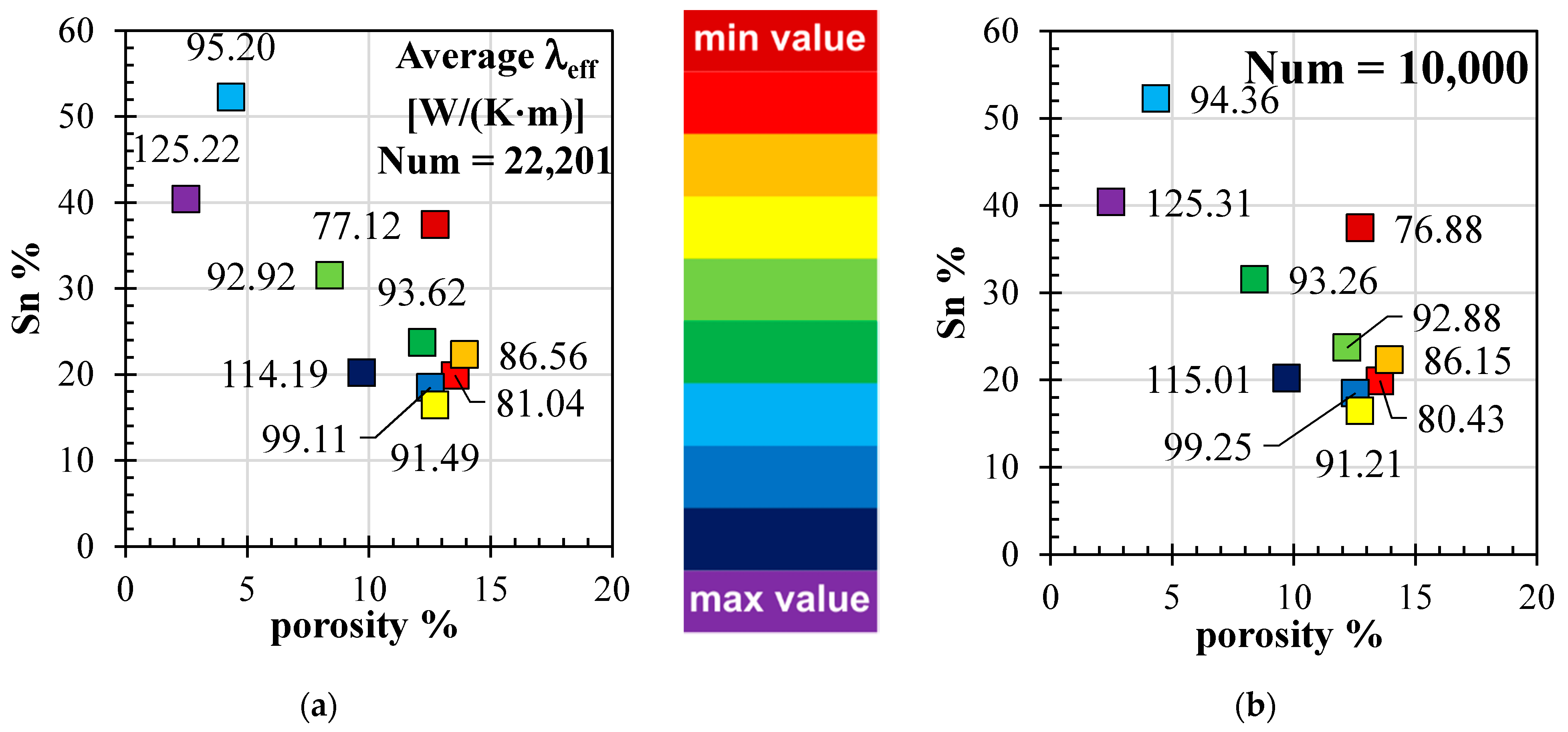
Effective thermal conductivity values are displayed as a function of Sn and porosity content in volume percent, according to the number of particles (Num) equal to 22,201 (Figure 6a) and equal to 10,000 (Figure 6b). The highest λeff, 125 W/(K·m), is observed for the lowest porosity content (2.49% volume) and for 40% Sn. It is difficult to identify a clear trend to correlate λeff values with Sn or porosity values.
The average value of λeff calculated over all the areas is 95.65 ± 14.52 W/(K·m) for Num = 22,201 and 95.47 ± 14.82 W/(K·m) for Num = 10,000.
Comparing λeff along horizontal and vertical directions of the selected regions of micrographs, values can be higher in the direction or, in the other direction, suggesting isotropic thermal conductivity, since the ratio between the difference of thermal conductivity in horizontal and vertical directions and the vertical one is less than 1%. Furthermore, since the orthotropic material microstructure was observed for produced samples, thermal conductivity in a perpendicular metallographic section would lead to values corresponding to those in a horizontal (x) direction.
4. Discussion
The validation of 2D-LMC method for two-phase materials with literature data and DS numerical simulation gave good results. Considering the overall trend for λeff, it reduces as Sn volume content increases as well as with temperature. The predicted thermal conductivities have a good agreement with experimental data at relatively low temperatures. At 460 K, the equilibrium Al-Sn phase diagram [29] suggests that the mutual solubility of the elements increases. It is known that the formation of solid solutions reduces the thermal conductivity with respect to those of metals. This could be the case for Al-Sn alloys, for which the experimental data presented by Reference [20] rapidly decrease above a certain temperature. In these conditions, the use of the thermal conductivity of Al and Sn cannot be considered anymore, since the two phases identified as black and white are not pure Al and pure Sn. The available data did not allow us to verify this explanation. The results show also that the material is likely to have an isotropic response in planes perpendicularly to the solidification axis of the sample from which micrographs have been taken by Reference [20].
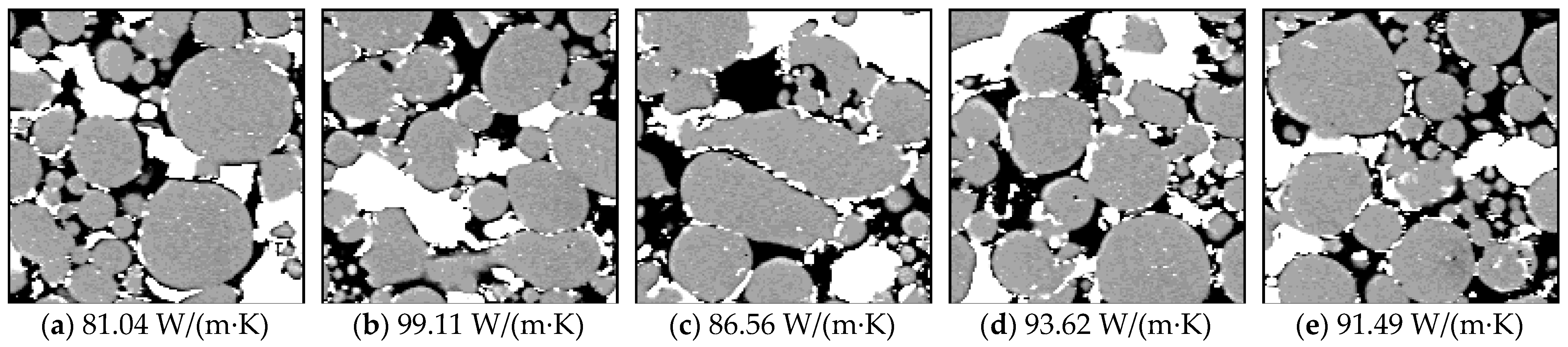
The application of the 2D-LMC method for three-phase analysis shows the effect of composition and morphology on effective thermal conductivity even more clearly. An increase of Sn and porosity volume fractions causes the reduction of λeff, with a predominant effect of porosity, as it can be easily expected. Nevertheless, even a slight variation of volume content of phases can give very different results. For example, this can be observed for about 12% of porosity and 20% of Sn in volume (Figure 7). Despite a very similar composition, these areas have a different phase distribution, which can explain differences up to 18% in the λeff value. Further studies are required to obtain a deep understanding on the role of the three phase distributions.
The reduction of the number of jumping particles provided almost the same results, only with a higher standard deviation. This aspect is particularly interesting for the use of the LMC method, since computational time, especially on images with many nodes, can be significantly reduced. Therefore, the present work suggests the repetition of the simulation on many areas sampled randomly for more cycles, but with a low number of jumping particles as a possible approach to apply the LMC method to real microstructures. In this way, the loss of precision induced by the small size of images and the low number of particles is balanced with the statistics on results.
The experimental λeff for Al-10vol%Sn is 76.863 ± 0.352 W/(m·K), while the average result of the LMC simulation is 95.65 ± 14.52 W/(K·m) (Num = 22,201). The standard deviation of the LMC simulations is very large. Thus, the experimental and simulation values can be considered to be similar. Moreover, since the sample was sintered at 500 °C, it is reasonable to expect the presence of mutual solute atoms, which reduce the actual thermal conductivity of the material with respect to the one calculated considering the thermal conductivity of pure Al and Sn, as mentioned above. The presence of impurities consisting of other elements could affect thermal conductivity of the phases as well. However, according to nominal composition of raw materials, impurity content should be very low and chemical analysis did not show significant quantities.
The use of LMC simulation proved to give the real effect of the three-phase microstructure with respect to analytical models. Considering a very simple example, for Al-10vol%Sn-8%vol%pores, if the upper and lower boundary rule of mixture is applied, the expected thermal conductivity should range from about 210 W/(K·m) to 0 W/(K·m). Therefore, the LMC provides a far closer estimation. Moreover, considering the presented microstructure, the application of analytical models where inclusions are represented as regular objects, like spheres or cylinders, would be a very rough approximation. The application of the LMC simulation in this case allows us to obtain a good estimation of effective thermal conductivity starting from a real microstructure, without the need for finite element analyses.
5. Conclusions
Effective thermal conductivity of composite metallic materials was evaluated both numerically and experimentally. The Lattice Monte-Carlo method was applied to estimate the effective thermal conductivity of two-phase and three-phase materials from micrographs. The validation with experimental data about Al-Sn alloys showed that the difference between numerical and experimental results is below 5% at relatively low temperatures. Less precise predictions, with variations up to 8%, can be observed if the alloy is heated above 450 K, due to mutual elements’ diffusion, which reduces thermal conductivity of each phase with respect to the corresponding pure element phases. Furthermore, the use of the LMC method, especially for three-phase material, highlighted the effect of morphology of phases in addition to local phase content. The LMC method proved to be a very effective tool for evaluating thermal conductivity of two- or three-phase composite materials, taking into account their real microstructure. These results can be applied in the development of composite materials for thermal applications, allowing us to study the effect of a specific microstructure on heat transfer. This is particularly interesting for application of binary alloys, like Al-Sn, as phase change materials for thermal energy management, for which thermal conductivity is one of the most important properties. Thanks to a deeper knowledge on the effect of microstructure on effective thermal conductivity, it would be possible to tailor the microstructure to obtain optimal heat transfer.
Author Contributions
Conceptualization, E.G. Data curation, Z.L. and C.C. Formal analysis, Z.L. and C.C. Investigation, C.C. Methodology, Z.L., C.C. and E.G. Project administration, E.G. Software, Z.L. and C.C. Supervision, E.G. Validation, Z.L. and C.C. Visualization, Z.L. and C.C. Writing—original draft, C.C. Writing—review & editing, Z.L. and E.G. All authors will be informed about each step of manuscript processing including submission, revision, revision reminder, etc. via emails from our system or assigned Assistant Editor. All authors have read and agreed to the published version of the manuscript.
Funding
The Italian Ministry of Education, University and Research is acknowledged for the support through the Project “Department of Excellence LIS4.0−Lightweight and Smart Structures for Industry 4.0”.
Institutional Review Board Statement
Not applicable.
Informed Consent Statement
Not applicable.
Data Availability Statement
The raw data required to reproduce these findings cannot be shared at this time as the data also forms part of an ongoing study. The processed data required to reproduce these findings cannot be shared at this time as the data also forms part of an ongoing study.
Acknowledgments
The authors would like to thank Alessandra Camnaghi for her help in thermodynamic calculations and experimental activities during her master’s thesis.
Conflicts of Interest
The authors declare no conflict of interest. The funders had no role in the design of the study, in the collection, analyses, or interpretation of data, in the writing of the manuscript, or in the decision to publish the results.
References
- Burger, N.; Laachachi, A.; Ferriol, M.; Lutz, M.; Toniazzo, V.; Ruch, D. Review of thermal conductivity in composites: Mechanisms, parameters and theory. Prog. Polym. Sci. 2016, 61, 1–28. [Google Scholar] [CrossRef]
- Meydaneri, F.; Saatçi, B.; Özdemir, M. Thermal conductivities of solid and liquid phases for pure Al, pure Sn and their binary alloys. Fluid Phase Equilib. 2010, 298, 97–105. [Google Scholar] [CrossRef]
- Rawson, A.J.; Kisi, E.; Wensrich, C. Microstructural efficiency: Structured morphologies. Int. J. Heat Mass Transf. 2015, 81, 820–828. [Google Scholar] [CrossRef]
- Rawson, A.; Kisi, E.; Sugo, H.; Fiedler, T. Effective conductivity of Cu-Fe and Sn-Al miscibility gap alloys. Int. J. Heat Mass Transf. 2014, 77, 395–405. [Google Scholar] [CrossRef] [Green Version]
- Progelhof, R.C.; Throne, J.L.; Ruetsch, R.R. Methods for predicting the thermal conductivity of composite systems: A review. Polym. Eng. Sci. 1976, 16, 615–625. [Google Scholar] [CrossRef]
- Veyhl, C.; Fiedler, T.; Andersen, O.; Meinert, J.; Bernthaler, T.; Belova, I.V.; Murch, G.E. On the thermal conductivity of sintered metallic fibre structures. Int. J. Heat Mass Transf. 2012, 55, 2440–2448. [Google Scholar] [CrossRef]
- Fiedler, T.; Löffler, R.; Bernthaler, T.; Winkler, R.; Belova, I.V.; Murch, G.E.; Öchsner, A. Numerical analyses of the thermal conductivity of random hollow sphere structures. Mater. Lett. 2009, 63, 1125–1127. [Google Scholar] [CrossRef]
- Karkri, M.; Ibos, L.; Garnier, B. Comparison of experimental and simulated effective thermal conductivity of polymer matrix filled with metallic spheres: Thermal contact resistance and particle size effect. J. Compos. Mater. 2015, 49, 3017–3030. [Google Scholar] [CrossRef]
- Fiedler, T.; Belova, I.V.; Rawson, A.; Murch, G.E. Optimized Lattice Monte Carlo for thermal analysis of composites. Comput. Mater. Sci. 2014, 95, 207–212. [Google Scholar] [CrossRef]
- Ye, H.; Ni, Q.; Ma, M. A Lattice Monte Carlo analysis of the effective thermal conductivity of closed-cell aluminum foams and an experimental verification. Int. J. Heat Mass Transf. 2015, 86, 853–860. [Google Scholar] [CrossRef]
- Fiedler, T.; Rawson, A.J.; Sugo, H.; Kisi, E. Thermal capacitors made from Miscibility Gap Alloys (MGAs). In WIT Transactions on Ecology and the Environment, Proceedings of the 5th International Conference on Energy and Sustainability, Putrajaya, Malaysia, 16–18 December 2014; WIT Press: Southampton, UK, 2014; Volume 186, pp. 479–486. [Google Scholar] [CrossRef]
- Belova, I.V.; Murch, G.E. Bridging Different Length and Time Scales in Diffusion Problems Using a Lattice Monte Carlo Method. Solid State Phenom. 2007, 129, 1–10. [Google Scholar] [CrossRef]
- Li, Z.; Gariboldi, E. Reliable estimation of effective thermal properties of a 2-phase material by its optimized modelling in view of Lattice Monte-Carlo simulation. Comput. Mater. Sci. 2019, 169, 109–125. [Google Scholar] [CrossRef]
- Gariboldi, E.; Colombo, L.P.M.; Fagiani, D.; Li, Z. Methods to Characterize Effective Thermal Conductivity, Diffusivity and Thermal Response in Different Classes of Composite Phase Change Materials. Materials 2019, 12, 2552. [Google Scholar] [CrossRef] [PubMed] [Green Version]
- Shinzato, K.; Baba, T. A Laser Flash Apparatus for Thermal Diffusivity and Specific Heat Capacity Measurements. J. Therm. Anal. Calorim. 2001, 64, 413–422. [Google Scholar] [CrossRef]
- ASTM International. E1461-13 Standard Test Method Thermal Diffusivity by the Flash Method; ASTM International: West Conshohocken, PA, USA, 2013. [Google Scholar] [CrossRef]
- Liu, X.; Zeng, M.Q.; Ma, Y.; Zhu, M. Promoting the high load-carrying capability of Al–20wt%Sn bearing alloys through creating nanocomposite structure by mechanical alloying. Wear 2012, 294–295, 387–394. [Google Scholar] [CrossRef]
- Sugo, H.; Cuskelly, D.; Rawson, A.; Erich, K. High conductivity PCM for thermal energy storage—Miscibility Gap Alloys. In Proceedings of the Solar2014: The 52nd Annual Conference, Australian Solar Energy Society (Australian Solar Council), Melbourne, Australia, 9 May 2014; pp. 201–210. [Google Scholar]
- Confalonieri, C.; Bassani, P.; Gariboldi, E. Microstructural and thermal response evolution of metallic form-stable phase change materials produced from ball-milled powders. J. Therm. Anal. Calorim. 2020, 142, 85–96. [Google Scholar] [CrossRef]
- Meydaneri Tezel, F.; Saatçi, B.; Arı, M.; Durmuş Acer, S.; Altuner, E. Structural and thermo-electrical properties of Sn–Al alloys. Appl. Phys. A 2016, 122, 906. [Google Scholar] [CrossRef]
- Rasband, W.S. ImageJ, Version 2.0.0-rc-69/1.52i, Distribution Fiji. 2018. Available online: https://imagej.net/Welcome (accessed on 29 March 2021).
- Li, Z.; Gariboldi, E. Review on the temperature-dependent thermophysical properties of liquid paraffins and composite phase change materials with metallic porous structures. Mater. Today Energy 2021, 20, 100642. [Google Scholar] [CrossRef]
- Gariboldi, E.; Perrin, M. Metallic Composites as Form-Stable Phase Change Alloys. Mater. Sci. Forum 2018, 941, 1966–1971. [Google Scholar] [CrossRef]
- Thermo-Calc Software. Version 2020b with TCAL5.1 Al-Alloys Database; Thermo-Calc Software: Stockholm, Sweden, 2020. [Google Scholar]
- Taylor, J.R. Introduzione All’Analisi Degli Errori, 1st ed.; Zanichelli: Bologna, Italy, 1986. [Google Scholar]
- Yamasue, E.; Susa, M.; Fukuyama, H.; Nagata, K. Deviation from Wiedemann–Franz Law for the Thermal Conductivity of Liquid Tin and Lead at Elevated Temperature. Int. J. Thermophys. 2003, 24, 713–730. [Google Scholar] [CrossRef]
- Bakhtiyarov, S.I.; Overfelt, R.A.; Teodorescu, S.G. Electrical and thermal conductivity of A319 and A356 aluminum alloys. J. Mater. Sci. 2001, 36, 4643–4648. [Google Scholar] [CrossRef]
- Baehr, H.D.; Stephan, K. Heat and Mass Transfer, 2nd ed.; Springer: Berlin/Heidelberg, Germany, 2006; ISBN 978-3-540-29526-6. [Google Scholar]
- Pilote, L.; Gheribi, A.E.; Chartrand, P. Study of the solubility of Pb, Bi and Sn in aluminum by mixed CALPHAD/DFT methods: Applicability to aluminum machining alloys. Calphad 2018, 61, 275–287. [Google Scholar] [CrossRef]
Figure 1.
Area of Al-10vol%Sn microstructure prepared for the Lattice Monte-Carlo (LMC) method: (a) Original cropped image and (b) three-zone image after application of a multi-threshold. The side of the micrograph is 80.54 µm in length.
Figure 1.
Area of Al-10vol%Sn microstructure prepared for the Lattice Monte-Carlo (LMC) method: (a) Original cropped image and (b) three-zone image after application of a multi-threshold. The side of the micrograph is 80.54 µm in length.

Figure 2.
(a) Effective thermal conductivity of Al-Sn alloys vs. Sn volume fraction experimentally measured by Meydaneri Tezel et al. [20] at 340 K and estimated by the Lattice Monte-Carlo (LMC) method and direct simulation (DS) method at the same temperature. In addition to average values of effective thermal conductivity, those obtained along the horizontal (x) and vertical, (y) direction in their micrographs are given. (b) Experimental and calculated effective thermal conductivity as a function of temperature data for pure Al, pure tin, and for different Al-Sn alloys.

Figure 3.
SEM micrograph of Al-10vol%Sn sample, sectioned on a plane parallel to the compression direction.
Figure 3.
SEM micrograph of Al-10vol%Sn sample, sectioned on a plane parallel to the compression direction.

Figure 4.
SEM micrograph for LMC simulations of Al-10vol%Sn sample, sectioned on a plane parallel to the compression direction.
Figure 4.
SEM micrograph for LMC simulations of Al-10vol%Sn sample, sectioned on a plane parallel to the compression direction.

Figure 5.
Comparison between results obtained with a different number of particles: 22,201 on the x-axis and 10,000 on the y-axis. The line is the bisector of the first quadrant of the plot (y = x).
Figure 5.
Comparison between results obtained with a different number of particles: 22,201 on the x-axis and 10,000 on the y-axis. The line is the bisector of the first quadrant of the plot (y = x).

Figure 6.
Average effective thermal conductivity (values next to datapoints). The color should help to order values from a minimum to a maximum. (a) Results with the number of particles (Num) equal to 22,201. (b) Results with the number of particles (Num) equal to 10,000.
Figure 6.
Average effective thermal conductivity (values next to datapoints). The color should help to order values from a minimum to a maximum. (a) Results with the number of particles (Num) equal to 22,201. (b) Results with the number of particles (Num) equal to 10,000.

Figure 7.
Regions of Figure 4 with about 12% porosity and 20% of Sn in volume and their average λeff (Num = 22,201). The side of each micrograph is 80.54 µm in length. (a–e) refer to different regions chosen from Figure 4 with their effective thermal conductivity.


Table 1.
Thermal conductivity values for Al and Sn at different temperatures inferred from the plot of experimental data provided in Reference [20].
Table 1.
Thermal conductivity values for Al and Sn at different temperatures inferred from the plot of experimental data provided in Reference [20].
| Phase | Thermal Conductivity [W/(m·K)] | ||
|---|---|---|---|
| at 340 K | at 400 K | at 460 K | |
| Al | 306.56 | 296.66 | 286.76 |
| Sn | 69.18 | 65.28 | 61.38 |
Table 2.
Calculated (Cp) or experimental (density and thermal diffusivity) values to determine thermal conductivity.
Table 2.
Calculated (Cp) or experimental (density and thermal diffusivity) values to determine thermal conductivity.
| Value | Density [g/cm3] | Cp [J/(g·K)] | Thermal Diffusivity [cm2/s] | Thermal Conductivity [W/(m·K)] |
|---|---|---|---|---|
| Average | 2.901 | 0.743 | 0.357 | 76.863 |
| Error (%) | 0.164 1 | - | 0.428 1 | 0.458 2 |
1 standard deviation% 2 experimental error (Equation (1)).
Publisher’s Note: MDPI stays neutral with regard to jurisdictional claims in published maps and institutional affiliations. |
© 2021 by the authors. Licensee MDPI, Basel, Switzerland. This article is an open access article distributed under the terms and conditions of the Creative Commons Attribution (CC BY) license (https://creativecommons.org/licenses/by/4.0/).
Share and Cite
MDPI and ACS Style
Li, Z.; Confalonieri, C.; Gariboldi, E. Numerical and Experimental Evaluation of Thermal Conductivity: An Application to Al-Sn Alloys. Metals 2021, 11, 650. https://doi.org/10.3390/met11040650
AMA Style
Li Z, Confalonieri C, Gariboldi E. Numerical and Experimental Evaluation of Thermal Conductivity: An Application to Al-Sn Alloys. Metals. 2021; 11(4):650. https://doi.org/10.3390/met11040650
Chicago/Turabian StyleLi, Ziwei, Chiara Confalonieri, and Elisabetta Gariboldi. 2021. "Numerical and Experimental Evaluation of Thermal Conductivity: An Application to Al-Sn Alloys" Metals 11, no. 4: 650. https://doi.org/10.3390/met11040650
Note that from the first issue of 2016, this journal uses article numbers instead of page numbers. See further details here.