A Stochastic Model Approach for Copper Heap Leaching through Bayesian Networks
by
 , , , and
Manuel Saldaña
1,* ,
,
Javier González
2, 
Ricardo I. Jeldres
3,
Ángelo Villegas
2,
Jonathan Castillo
4 ,
,
Gonzalo Quezada
5 and
and
Norman Toro
2,6,* 1
Departamento de Ingeniería de Sistemas y Computación, Facultad de Ingeniería y Ciencias Geológicas, Universidad Católica del Norte, 1270709 Antofagasta, Chile
2
Departamento de Ingeniería Metalúrgica y Minas, Facultad de Ingeniería y Ciencias Geológicas, Universidad Católica del Norte, 1270709 Antofagasta, Chile
3
Departamento de Ingeniería Química y Procesos de Minerales, Facultad de Ingeniería, Universidad de Antofagasta, 1270300 Antofagasta, Chile
4
Departamento de Ingeniería en Metalurgia, Universidad de Atacama, 1531772 Copiapó, Chile
5
Water Research Center for Agriculture and Mining (CRHIAM), University of Concepción, 4030000 Concepción, Chile
6
Department of Mining and Civil Engineering, Polytechnic University of Cartagena, 30203 Cartagena, Spain
*
Authors to whom correspondence should be addressed.
Metals 2019, 9(11), 1198; https://doi.org/10.3390/met9111198
Submission received: 14 October 2019
/
Revised: 21 October 2019
/
Accepted: 4 November 2019
/
Published: 7 November 2019
(This article belongs to the Special Issue Advanced Simulation Technologies of Metallurgical Processing)
Abstract
:Multivariate analytical models are quite successful in explaining one or more response variables, based on one or more independent variables. However, they do not reflect the connections of conditional dependence between the variables that explain the model. Otherwise, due to their qualitative and quantitative nature, Bayesian networks allow us to easily visualize the probabilistic relationships between variables of interest, as well as make inferences as a prediction of specific evidence (partial or impartial), diagnosis and decision-making. The current work develops stochastic modeling of the leaching phase in piles by generating a Bayesian network that describes the ore recovery with independent variables, after analyzing the uncertainty of the response to the sensitization of the input variables. These models allow us to recognize the relations of dependence and causality between the sampled variables and can estimate the output against the lack of evidence. The network setting shows that the variables that have the most significant impact on recovery are the time, the heap height and the superficial velocity of the leaching flow, while the validation is given by the low measurements of the error statistics and the normality test of residuals. Finally, probabilistic networks are unique tools to determine and internalize the risk or uncertainty present in the input variables, due to their ability to generate estimates of recovery based upon partial knowledge of the operational variables.
1. Introduction
Copper mining is a constantly growing industry [1], and in countries like Chile, this industry represents 10% of the gross national product (GNP) [2], while approximately 19.7 million tons are produced annually worldwide [3]. Among the copper ores on the planet, the vast majority correspond to sulfured minerals, and a smaller amount to oxidized minerals [4], which is why flotation techniques and smelting processes are used to process these minerals, and to a lesser extent hydrometallurgical techniques [5]. However, flotation techniques generate a large amount of waste, resulting in tailings and the generation of acid drainage by the oxidation of minerals with a high presence of pyrite [4,6].
On the other hand, pyrometallurgical processes produce high emissions of sulfur dioxide (SO2), which together with NOx and CO2, can cause major problems, such as acid rain and increased local pollution [5]. So, hydrometallurgy is a good alternative to process both oxidized minerals and sulfurized minerals, since it is more environmentally friendly [5,7,8].
During the last 50 years, heap leaching processes were a very attractive technological option for the treatment of low grade minerals, allowing the economic exploitation of marginal deposits, often in remote locations in many parts of the world [9]. They are applied to previously crushed minerals in crushers, where the copper (Cu) present in the mineralized rock is extracted by the mixture between water and leaching agents [10]. This process is performed in leaching piles, where its typical height is between 4 to 10 m, although in some cases they can reach 18 m [11]. It can be applied for oxidized copper ores of low to medium grades (0.3–0.7%) as well as secondary copper sulfides. In heap leaching, larger sizes generally range between 10 and 40 mm, where sizes less than 6 mm are unacceptable, because they affect the permeability of the pile, especially if there are clayey minerals that result in a greater obstruction of heaps over time, due to swelling and gradual decrepitation. The leaching solution is distributed on top of the heap by sprinklers or drip emitters and then flows down through the heap under gravity. The volumetric flows of the typical solution vary between 4 and 20 L/(h × m2) [9]. Finally, cupric ions (Cu2+) are obtained together with other ions of elements dissolved in the pregnant liquid solution (PLS), which ions all advance to the subsequent stage of solvent extraction [12].
In the present investigation, the modeling of the copper heap leaching process is proposed using a stochastic approach through bayesian networks (BN), which considers both the distributions of the independent variables and the conditioned distributions of the response variable to the independent variables, in addition to the conditional relationships between the independent variables. The generation of this type of model allows investigation of the effects of the variables or input factors on one or more output variables through intentional changes, which are used to identify the conditions of the process and its components that affect the extraction behavior, in order to identify the configuration of factors that have a greater conditional dependence on the response variable. On the other hand, the modeling of this type of processes, in addition to being efficient in predicting the response variable, is robust to the lack of evidence; that is, they have the capacity to estimate recovery under conditions of lack of evidence or lack of knowledge, or more independent variables.
2. Materials and Methods
2.1. Machine Learning
Machine Learning is related to the creation of computer programs or algorithms which automatically improve and/or adapt their performance through experience. Machine learning has many things in common with other domains, such as statistics and probability theory (understanding of the phenomena that have generated the data), data mining (finding patterns in data that are understandable to people) and cognitive sciences (human learning aims to understand the mechanisms that underlie the various learning behaviors exhibited by people, such as concept learning, skill acquisition, strategy change, etc.) [13]. The objective of machine learning is to devise learning algorithms that automatically learn without human intervention or assistance, generating methods by which the computer creates its own program based on the examples we provide [14].
As part of the exploration and understanding of a process, ways of quantifying the events associated with its variables are sought. Depending on their complexity, these events could be associated with a single variable or multiple of them, and often follow an orderly, sequential evolution that could converge in one or more patterns that reflect, and sometimes determine, their behavior.
2.2. Data-Based Modeling in Mineral Processing
Machine learning and artificial intelligence techniques have a growing presence and impact in a wide variety of research fields. McCoy and Auret [15] develop a review of the state of machine learning applications in mineral processing. Data-based modeling methods in the mineral processing literature are frequently applied as “soft sensors” for the prediction of variables measured infrequently (or difficult to measure), based on variables measured frequently [16,17,18]. Some applications include the prediction of indicators of the grinding phase, determining the chemical properties that have a greater impact on the milling capacity indices by configuring an artificial neural network [19,20] or a regression of support vectors [21], Martin et al. [22]. On the other hand, they apply Random Forest (RF) for the prediction of the Hardgrove Grindability Index (HGI) based on a wide range of Kentucky coal samples.
Modeling applications to predict mill performance indicators based on process measurements, include the use of multivariate statistical methods such as partial least squares (PLS) and radial-based neural networks (RBF), demonstrating that the density of mill pulp and ball loading volume can be estimated reliably from different operational characteristics [23]. Ahmadzadeh and Lundberg [24], on the other hand, developed a method that predicts the remaining lifespan of a mill’s lining without stopping it, by modeling an artificial neural network capable of recognizing the complex relationships between inputs and departures. The results obtained by Ahmadzadeh and Lundberg [24] show a remarkably high degree of correlation between the input and output variables. The performance of the neural network model is very consistent for the data used for training and testing.
Other studies show the application of machine learning techniques to the prediction of flotation performance indicators based on process measurements. Jahedsaravani et al. [25] analyzed and modeled the relationship between flotation process conditions and foam characteristics through the use of neural networks. Similar to the study developed by Jahedsaravani et al., Massinaei and Doostmohammadi [26] studied the relationship between gas dispersion in a flotation cell and flotation speed using artificial neural network (ANN) techniques and statistics (nonlinear regression). Nakhaei et al. [27], investigates the prognosis of metallurgical performance (grade and recovery) of the flotation column of the pilot plant using artificial neural networks (ANN) and multivariable nonlinear regression (MNLR).
However, most of these neural networks applied to the modeling of mineral processes have to be relatively small, often with only a hidden layer due to computer or data limitations. Recent developments in the design and training of deep and complex neural networks have not been demonstrated in the literature on mineral processing. Comparisons between neural networks and methods such as linear or nonlinear regression have not confirmed a significant benefit of neural networks compared to simpler methods [26,27].
Wang et al. [28], developed another work that implements an interesting adaptive modeling application, where multiple neural networks are used to predict foam properties based on the measurements of input or feed parameters. As machine learning techniques become increasingly accessible as part of software packages, data-based modeling applications are likely to become more common and make use of more advanced techniques and analysis. In particular, techniques for modeling the dynamics of complex processes may be of interest, since most applications currently assume that observations are independent [15].
2.3. Bayesian Networks
The Bayesian networks model is a phenomenon through a set of variables with dependency relationships between them. In this model, Bayesian inference can estimate the subsequent probability of the unknown variables based on the known variables. These models can have different applications for classification, prediction, diagnosis, etc. In addition, they can give interesting information, as to how the domain variables are related, which can sometimes be interpreted as cause-effect relationships. A Bayesian network is therefore a device of representation destined to organize knowledge about a particular situation in a coherent whole. The Bayesian network is a graphical modeling tool to specify probability distributions [29].
Bayesian networks provide a graphical representation for a set of random variables and for the relationships between them. The structure of the network makes it possible to specify the joint probability function of these variables as the product of conditional probability functions, usually simpler ones. BN are probabilistic, multivariate models that relate a set of random variables through a directed graph that explicitly indicates causal influence and this is thanks to its probability update engine, Bayes’ Theorem [30]. Bayesian networks are an extremely useful tool in estimating probabilities to new evidence. A Bayesian network is, therefore, a type of causal network.
Then, defining the fundamentals of Bayesian networks, given a vector of random variables , a joint probability measure is defined (Equation (1)):
where . If the joint probability is known, it is possible to calculate any probability on the variables . Then the following propositions are defined: Rule of total probability (Equation (2)) and rule of marginalization (Equation (3)).
Then the theorem shown in Equation (2) shows a simple but powerful relationship between conditional probabilities, which will be the basis of Bayesian network theory.
where,
Now, considering the independence between the factors, the two random variables are independent if and only if the conditions of Equation (9) are met, or the condition of Equation (10) is met if the existence of evidence is considered.
If, on the contrary, X and Y are independent, o . The independence between variables allows a reduction in the complexity of the joint probability function, and instead of modeling a single function, we separate them into simpler parts.
Then, assuming that you have the data of the form , where C is the class variable, and you are looking to predict the value of the class a probabilistic approach will assign the most probable class (Equation (11)), which is:
Then, if Bayes’ Theorem is applied, the following is obtained (Equation (12)):
However, for the purpose of estimating the output, the expected value of mineral recovery through the product between the outputs and their conditional probabilities is considered, as shown in Equation (13).
where X represents the set of independent variables influencing the response variable in different degrees, and corresponds to a possible state of recovery in a given time t.
If the existence of certain independent variables is unknown, the expected value of the probability of each value of the response variable is considered conditional on the evidence of the n –k independent variables known and the conditional distributions of the k independent variables unknown, as shown in Equation (14).
It should be noted that the expected value of the k variables whose evidence is unknown may or may not be conditioned on the other independent variables, which is the variables whose evidence is known and the conditional distributions of the variables whose evidence is unknown.
2.4. Uncertainty Analysis
The uncertainty analysis (UA) corresponds to determine the uncertainty in the output variables as a result of the uncertainty in the input variables [31]. The UA is generally performed using the probability theory [32], where uncertainty is represented by the probability distribution functions (PDFs), and which can be done in four steps. First, the type of PDF and the magnitude of the uncertainty for each input variable is determined. In other words, the uncertainty of entry is characterized. Then, for each input variable, a sample of the PDF is generated. Third, the values of the output variables are determined for each element of the sample. Finally, the results are analyzed using graphs, descriptive statistics and statistical tests to characterize the behavior of the output variables.
When the input variables have epistemic uncertainties, the uncertainty can be represented by a uniform distribution. Design and operation variables present this type of uncertainty. When the input variables have stochastic uncertainties, the normal distribution is generally used to represent this type of uncertainty [33].
3. Results and Discussion
The results are ordered into three subsections: The results of the UA, which address the UA in the response variable at 30, 60 and 90 days of leaching; the modeling results of the copper recovery from the heap leaching process through the Bayesian networks, in addition to the conditional relationships between the independent variables and the recovery, and the conditional dependence between the independent variables, together with the degree of strength of the dependencies (reflected in the arcs that connect the nodes of the network). Finally, the effectiveness of the Bayesian network is studied as a tool to model the productive process of heap leaching, by calculating the indicators of goodness of adjustment mean absolute deviation (MAD), mean squared error (MSE) and mean absolute percentage error (MAPE), together with tests of the normality of the residues when evaluating the value expected response to changes in input variables and ignorance of one or more independent variables.
3.1. Analysis of Uncertainty
Equation (14) indicates that copper recovery depends on the operational variables’ sampled time, particle radius, pile height, particle porosity, surface velocity of the leaching flow and effective diffusivity of the solute through the pores of the particle.
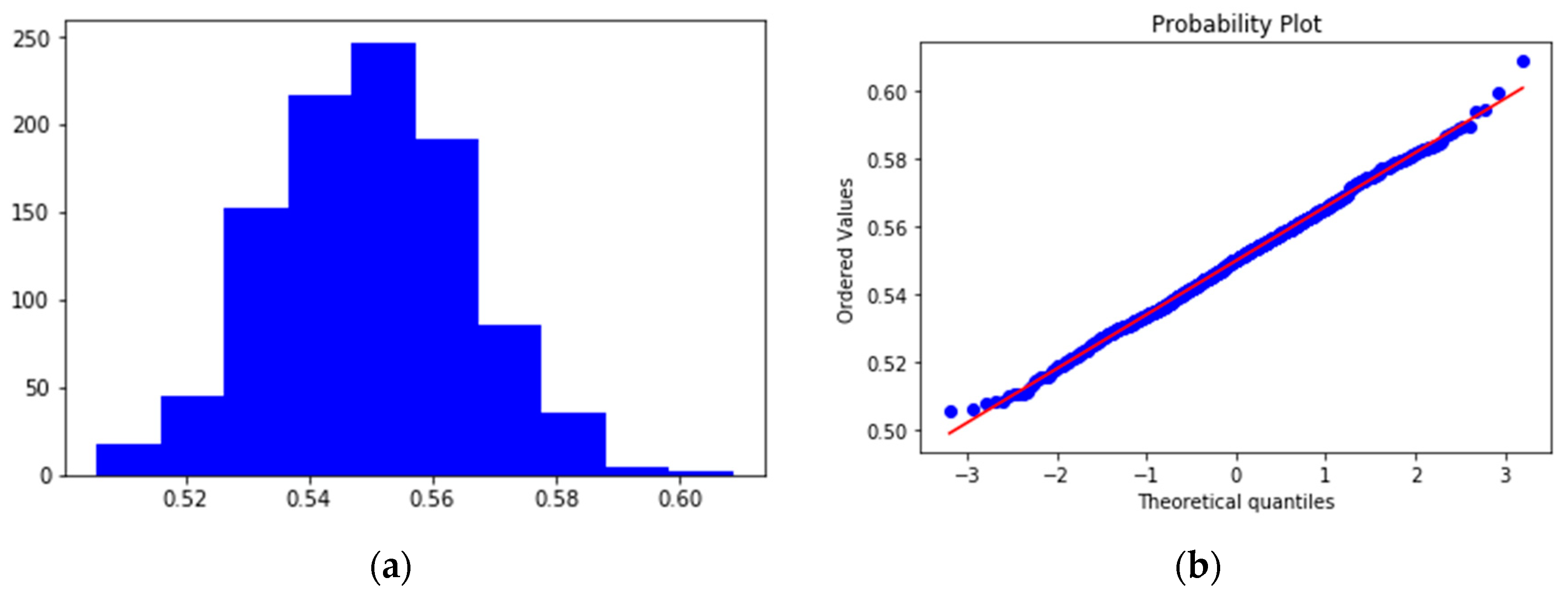
A good distribution function to represent epistemic uncertainties is the uniform PDF, taking the values of as the central tendency values of the parameters , respectively. The sensitivity analysis was analyzed three times for the occasions of 30, 60 and 90 days of leaching. The results are shown in Figure 1, Figure 2 and Figure 3, respectively.
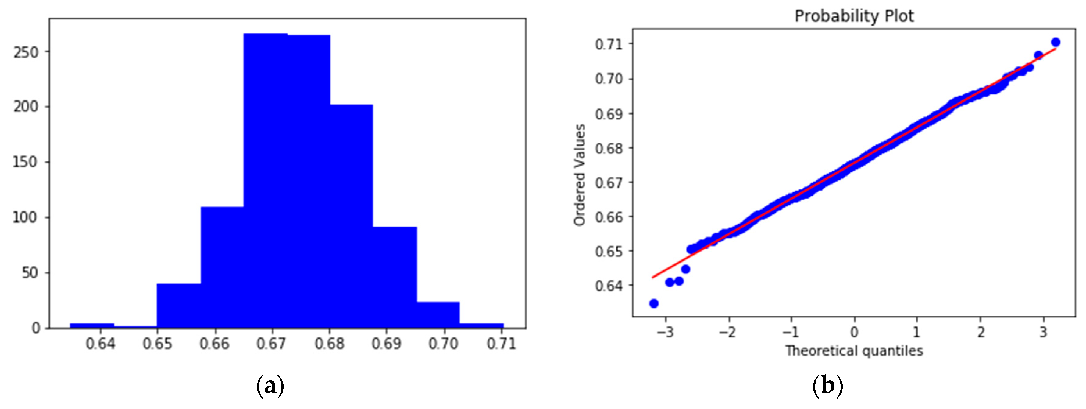
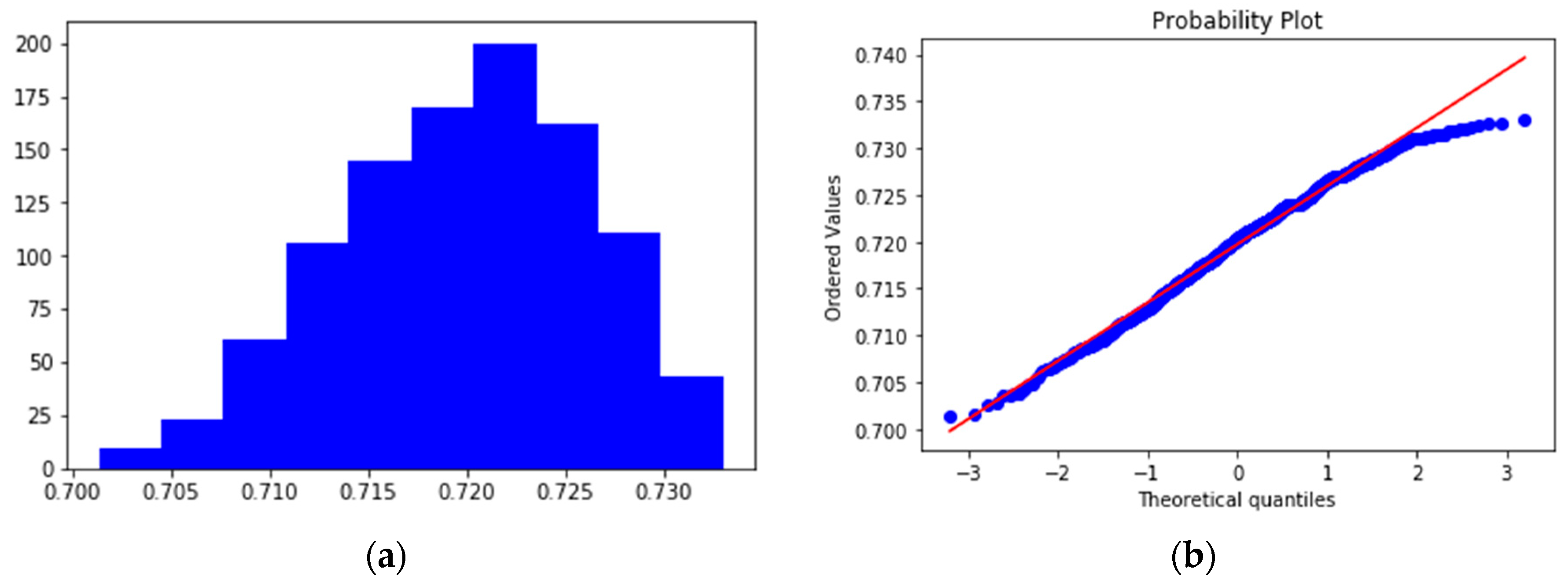
Figure 1, Figure 2 and Figure 3 show that the leaching time affects the kinetic uncertainty of the battery leaching phase. Histograms show that uncertainty in the input variables produces greater uncertainty in recovery after 30 days compared to uncertainty after 60 days, in addition to greater uncertainty after 60 days compared to sampling after 90 days leaching.
The normal probability plot (Figure 1b) indicates that when the leaching time is equal to 30 days, the recovery presents a normal PDF with a standard deviation of 1.75 and an average of 54.89% recovery, while when the leaching time is 60 days (Figure 2b), the recovery presents a normal PDF with an average of 57.53% and a deviation of 1.03.
On the other hand, the normal probability plot indicates that when the leaching time is equal to 90 days, the recovery has a tail that moves away from normal behavior. These results show that the Bayesian network can estimate the expected recovery of copper from heap leaching, considering a wide range of the uncertainties of independent variables. The change in the recovery behavior as a function of the time factor is because the recovery tends to present asymptotic behavior at high values of the time factor. It is evident that regardless of the value of the other independent variables, the deviation of the long-term recovery is less than at lower levels of the time factor.
3.2. Bayesian Network Modeling
The analysis of the behavior or dynamics of battery leaching involves a complex and multidimensional system in an environment, in which there is regularly uncertainty and the lack or absence of certain risk factors involved in the problem. The modeling made possible through probability distributions amid uncertainties, provided by the BN-based models, becomes appropriate to model the recovery of copper, considering that it allows one to deduce hypotheses and establish the relationships between the explanatory factors of the response variable. However, risk is a changing fact when it comes to time (among other aspects), and modeling through BNs satisfies this logic, since it stimulates stochastic processes [34].
The parameters’ leaching time, pile height, particle size, surface velocity of the leaching flow through the bed, effective diffusivity of the solute within the pores of the particle and the porosity of particle, were considered for the generation of the Bayesian network, information obtained from operational data from a mine in the Antofagasta region, Chile (data provided by the national mining company, Antofagasta, Chile, ENAMI, by its acronym in Spanish). The minimum, maximum and average values of the variables considered are presented in Table 1.
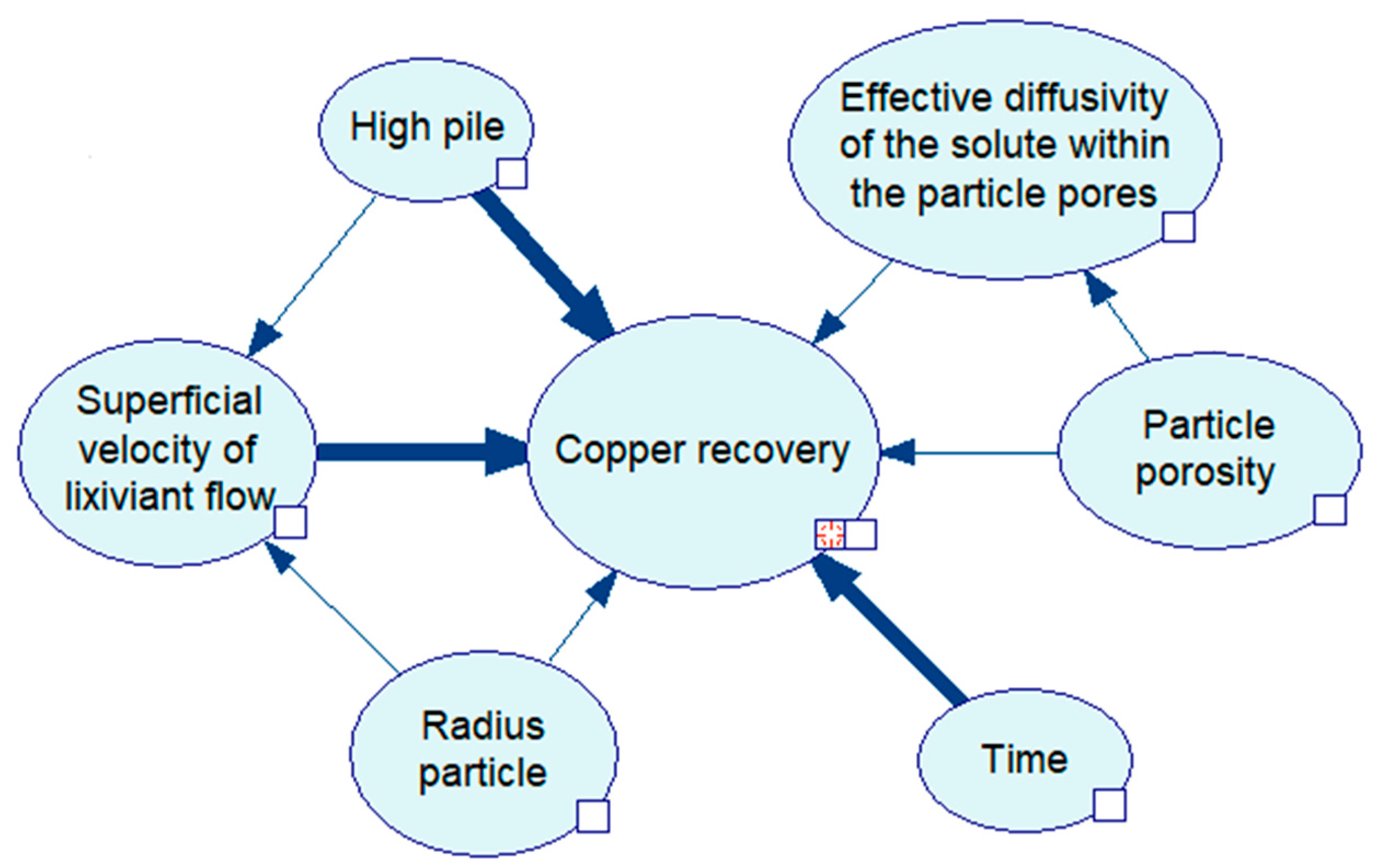
Developing the Bayesian network in GeNIe software (version 2.3) [35], the a priori structure of the network is given by Figure 4, where it is possible to appreciate that copper recovery is conditionally dependent upon all the variables considered in the sampling. Looking at the arches of the Bayesian network of Figure 4, they have a different thickness, indicating the force of influence between the nodes of the network. Strength of influence is always calculated from the total conditional probability (TCP) of the child node, and essentially expresses some form of distance between the various conditional probability distributions over the child node conditional on the states of the parent node; that is, the greater the thickness of the arc, the greater the conditional dependence between the nodes. The distance function that is used for the generation of the Bayesian network is the Euclidean function.
Once the network structure is identified, the probabilistic and computational calculations make the inference of the quantitative parameters of the model, with a possible interaction of the theoretical knowledge of the experts on the risk scenario that involves a specific problem, with the establishment of relationships that theoretically influence the response variable. Therefore, for the construction of analytical models using BN, prior subjective knowledge is required, which is also associated with the fact that the algebra of Bayesian analysis is more complex than classical analysis, especially in multidimensional problems.
Analyzing the network of Figure 4, it is necessary that the class variable “Copper recovery” is conditionally dependent on the independent variables considered in the sampling. However, for the set of sampled values, there is no conditional dependence between the variables that explains the answer. Then, incorporating a priori knowledge of the dynamics of the process handled by the authors (dependence relationships), the expected recovery following a stochastic approach should be modeled as shown in Figure 5.
Developing an analysis of influences of the nodes that show conditional dependence, prior to the establishment of relationships generated based on a priori knowledge managed by the system, the arcs that have a greater conditional dependence are time-copper recovery, heap height-recovery and superficial velocity of the leaching flow-recovery. Analyzing the Bayesian network outputs, the increase in the height and size of the typical commercial heap has not occurred simply as a result of economic efficiency but is also a function of the available surface area [9]. One of the factors that most influences the kinetics of the process is the percolation rate, which is directly related to the height of the pile and the permeability of the pile [12]. While time is a factor that greatly influences in copper recovery percentage from conventional leaching stacks, the current laws have made other technologies not profitable, since they require greater comminution or temperature [12].
For this reason, it works with long operating times, which may vary depending on the material to be worked and the recovery standards that the mining company is looking for.
On the other hand, the factors that have a marginal effect are the effective diffusivity of the solute within the pores of the particle and the size and porosity of particle. The influence force is always calculated from the total conditional probability (TCP) of the secondary node and essentially expresses some form of distance between the various distributions of conditional probability over the secondary node, conditioned on the states of the primary node.
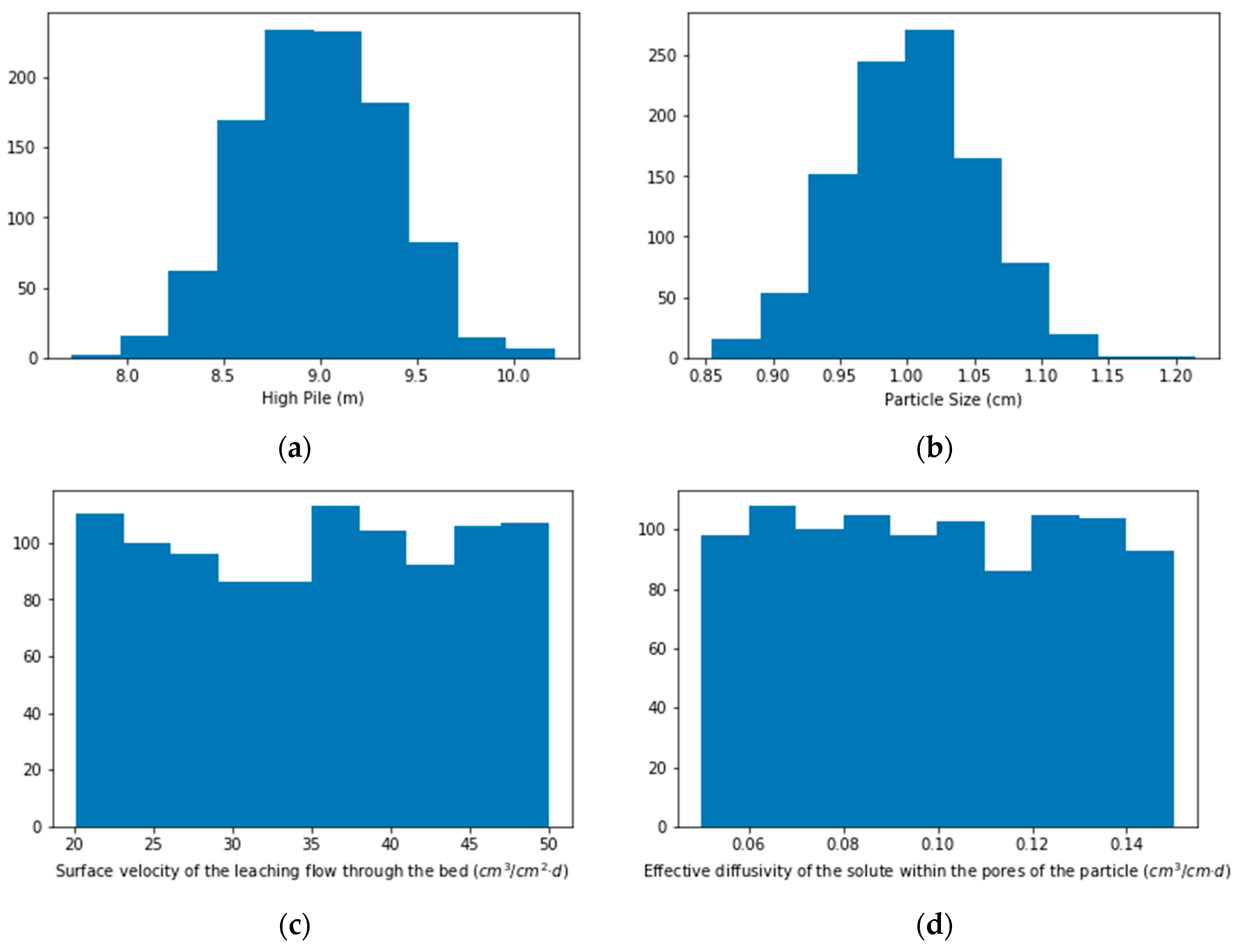
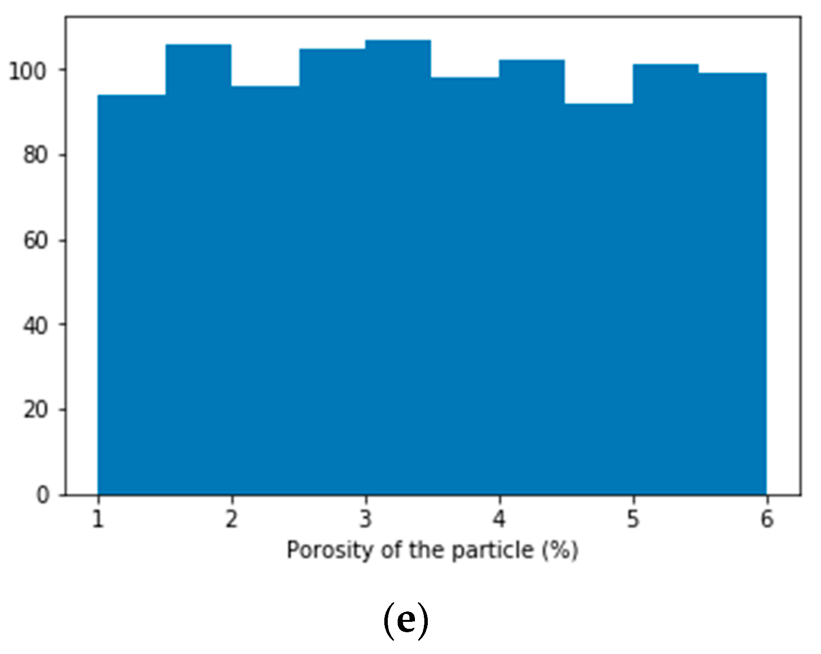
The total probability distributions identified by the Bayesian network are presented in Figure 6, where it can be seen that the stack height and particle size factors tend to be distributed normally (Figure 6a,b), while the surface velocity of the leaching flow (Figure 6c), the effective diffusivity of the solute through the pores of the particle (Figure 6d) and the porosity of the particle (Figure 6e) can be adjusted to a uniform continuous distribution. It is assumed that the time factor, as it is an operational sampling data, is uniform discrete, with a priori known values.
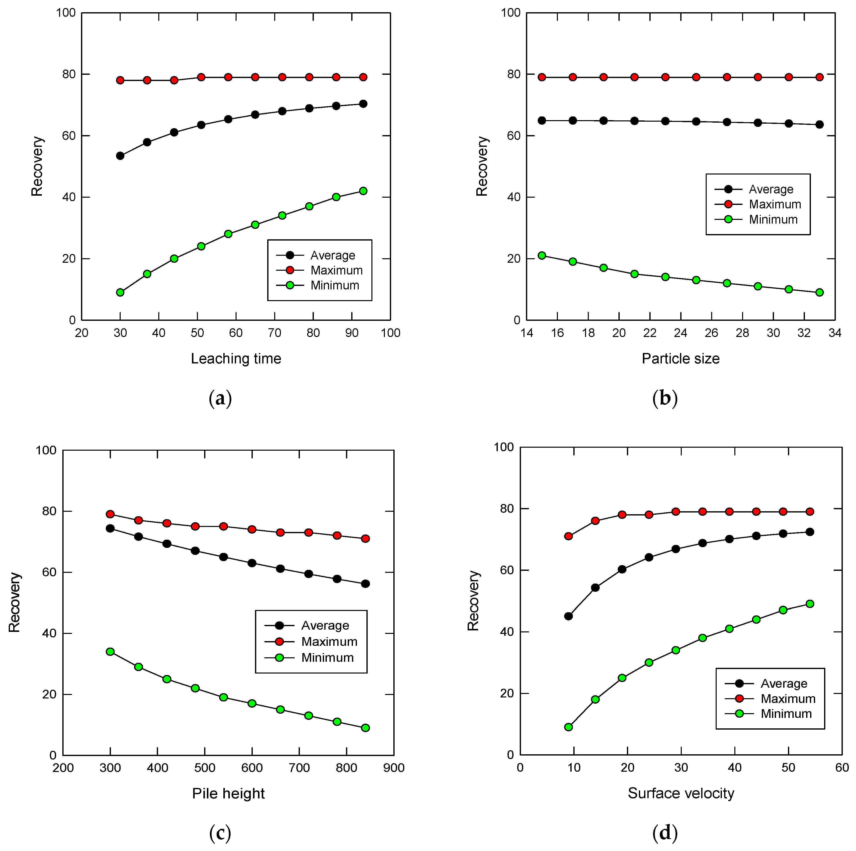
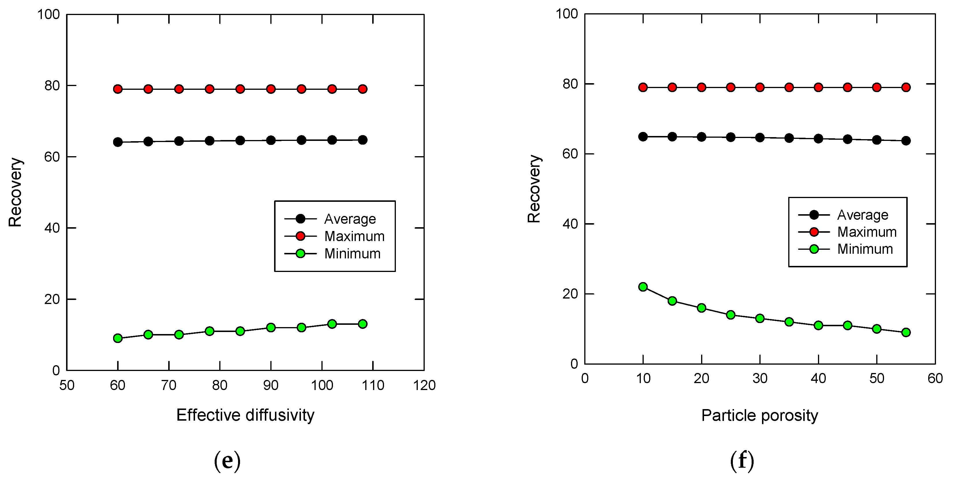
Then, the effectiveness of the Bayesian network is evaluated to estimate copper recovery considering a priori knowledge of the sampled parameters. The ability to predict the recovery is based on the knowledge of the n variables of interest, or the expected value of the response variable is calculated based on the underlying distributions of the independent variables unknown, while the dynamics of the recovery based on each of the independent variables is presented in Figure 7.
3.3. Bayesian Network Validation
Finally, the effectiveness of the Bayesian network is evaluated to estimate copper recovery considering a priori knowledge of the parameters considered in its generation. The ability to predict recovery is based upon the knowledge of the n variables of interest, otherwise the expected value of the response variable is calculated conditioned on the underlying distributions of the independent variables, which in turn are conditioned on the evidence of the other independent variables already known. Then, the independent variables are sensitized, in order to estimate the expected recovery of ore, according to the stochastic model shown in Equation (14).
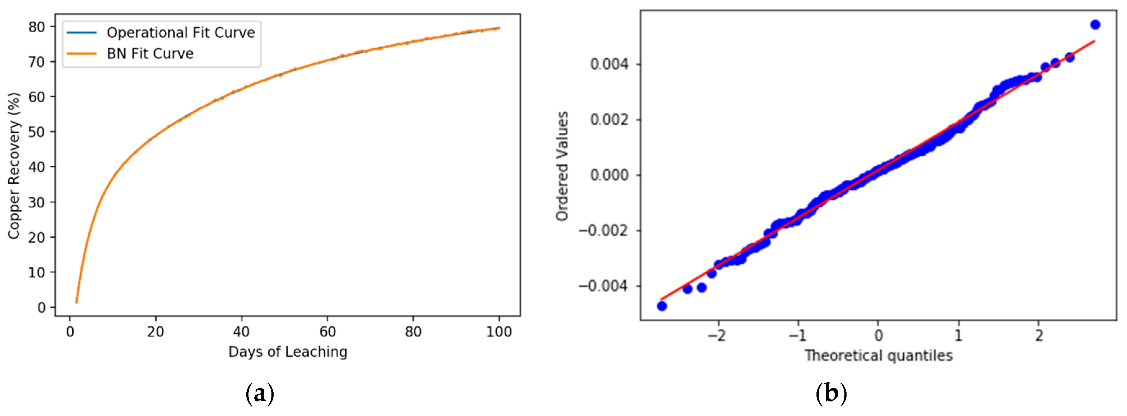
Estimating the recovery of copper through the Bayesian network adjusted with operational data from a copper mine considering as evidence the n independent variables, and analyzing the contrast between the outputs of the network and the operational results, as shown in Figure 8a, The Bayesian network presents a good fit to the operational data, and the goodness of fit statistics shown in Table 2 validate it.
On the other hand, Figure 8b shows that the assumption of the normality of the residues obtained from the contrast between the expected value of the network output and the operational data is reached, making the p-value of the test greater than the level of significance (p > 0.05), which indicates that the mathematical model is relatively accurate in representing the experimental design, although some points away from the line imply a distribution with outliers.
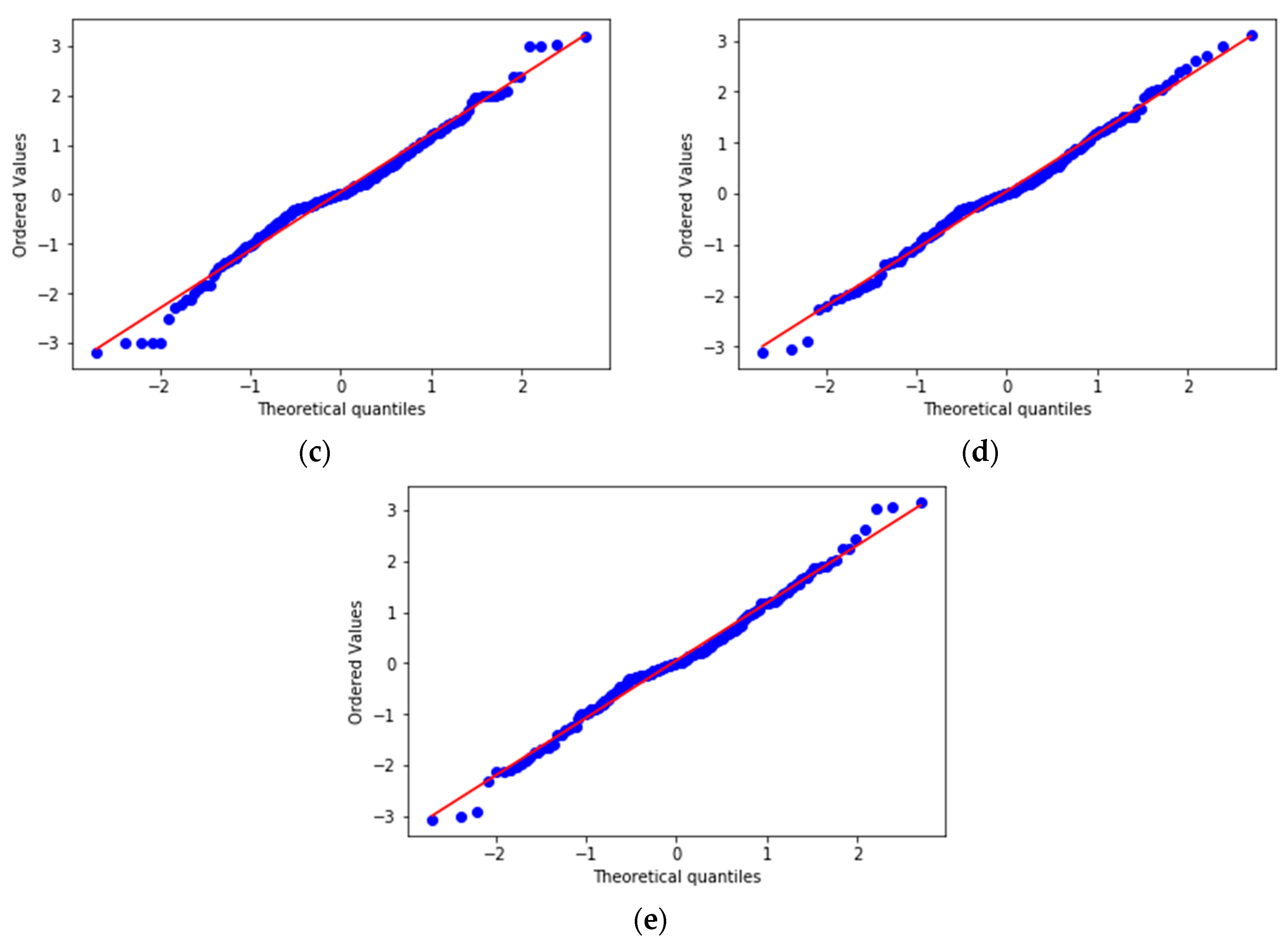
Analyzing the outputs of Bayesian networks over time and the variables defined by the nodes that represent the other independent variables, the expected value of the response is based on the evidence and the conditional distribution of the variable whose evidence is unknown. The expected recovery value obtained by the network is adjusted to the operational data, which is validated with the statistic p (p > 0.05), as shown in Figure 9.
The analysis of the residues between the experimental values and the expected recovery values generated by the network that excludes the knowledge of the porosity variables (Figure 9a) and the superficial velocity of the leaching flow (Figure 9b) do not present a normal adjustment, which together with high values of the goodness of fit indicators presented in Table 3 ratify the importance of both variables in the response.
In the opposite case, the residuals of the variables particle size (Figure 9c), effective diffusivity of the solute within the pores of the particle (Figure 9d) and porosity of the particle (Figure 9e) tend to have a normal adjustment (p = 0.05), indicating that these variables do not have a significant impact on recovery.
Following the example of Saldaña et al. [10], the generated stochastic model can be incorporated into a simulation framework that can quantify the benefits derived from the incorporation of probabilistic models in estimating the expected value of mineral recovery, or it could have the potential to include it in a system of support for decision making in the mining industry, as presented in Saldaña et al. [36].
4. Conclusions and Future Works
4.1. Conclusions
Probabilistic networks have become unique tools to determine and internalize the risk or uncertainty present in the input variables, and the importance of these is due to the ability to provide data for monitoring, as new information is added or removed from its structure, and also, for incorporate various hypotheses. Therefore, one of the main benefits of the Bayesian approach is the ability to incorporate prior information to quantify uncertainties and verify the legitimacy of the propositions.
Based on the above, it can be concluded that the behavior of the classification algorithms based on Bayesian networks presents satisfactory results in general terms, since the error obtained in the classification is minimal, which is validated by the normalization statistics of adjustment and the normality of the residuals distribution.
The construction of the Bayesian network model to analyze the dynamics of the leaching process has the potential to contribute to:
- Identifying the dependency relationships between independent variables and the response variable, in addition to dependency relationships between independent variables.
- Determining the variables that contribute most to explain the variability of the response.
- Assimilating quantitative knowledge in terms of the frequency of the occurrence of a given event (or level of recovery), using the parameters obtained by the BN, which will allow the identification of recurrent scenarios.
- The generation of copper recovery estimates based on partial knowledge of the operational variables considered in the study.
Finally, the variables that have a greater conditional dependence on the response variable are the time (mainly), the height of the stack and the superficial velocity of the leaching flow, while the variables that have a less significant impact are particle size, the porosity of the particle and the effective diffusivity of the solute within the pores of the particle.
4.2. Future Works
To further advance the operational investigation of leaching processes through a stochastic approach, sensitization of the variables of interest through a global sensitivity analysis are being considered. In addition, there is the incorporation into the stochastic model of the variability of the feeding of the productive process, and this will be through the generation of geostatistical models that relate the mineralogical content of the mine with the planning of extraction.
Author Contributions
M.S. and N.T. contributed in the methodology, conceptualization and modeling; J.G. and Á.V. investigation, writing review and editing; J.C. data curation and formal analysis and R.I.J. and G.Q. contributed with supervision and validation.
Funding
This research received no external funding.
Acknowledgments
Gonzalo Quezada and Ricardo Jeldres thank the Centro CRHIAM Project Conicyt/Fondap/15130015.
Conflicts of Interest
The authors declare no conflict of interest.
References
- Brininstool, M. Mineral Commodity Summaries: Copper; US Geological Survey: Reston, VA, USA, 2015.
- Pérez, K.; Toro, N.; Campos, E.; González, J.; Jeldres, R.I.; Nazer, A.; Rodriguez, M.H. Extraction of Mn from black copper using iron oxides from tailings and Fe2+ as reducing agents in acid medium. Metals 2019, 9, 1112. [Google Scholar] [CrossRef]
- Sulfuros primarios: Desafíos y oportunidades. Available online: https://www.cochilco.cl/Listado%20Temtico/sulfuros%20primarios_desaf%C3%ADos%20y%20oportunidades.pdf (accessed on 21 October 2019).
- Toro, N.; Briceño, W.; Pérez, K.; Cánovas, M.; Trigueros, E.; Sepúlveda, R.; Hernández, P. Leaching of pure chalcocite in a chloride media using sea water and waste water. Metals 2019, 9, 780. [Google Scholar] [CrossRef]
- Velásquez-Yévenes, L.; Torres, D.; Toro, N. Leaching of chalcopyrite ore agglomerated with high chloride concentration and high curing periods. Hydrometallurgy 2018, 181, 215–220. [Google Scholar] [CrossRef]
- Toro, N.; Saldaña, M.; Gálvez, E.; Cánovas, M.; Trigueros, E.; Castillo, J.; Hernández, P.C. Optimization of parameters for the dissolution of mn from manganese nodules with the use of tailings in an acid medium. Minerals 2019, 9, 387. [Google Scholar] [CrossRef]
- Pradhan, N.; Nathsarma, K.C.; Srinivasa Rao, K.; Sukla, L.B.; Mishra, B.K. Heap bioleaching of chalcopyrite: A review. Miner. Eng. 2008, 21, 355–365. [Google Scholar] [CrossRef]
- Castillo, J.; Sepúlveda, R.; Araya, G.; Guzmán, D.; Toro, N.; Pérez, K.; Rodríguez, M.; Navarra, A. Leaching of white metal in a NaCl-H2SO4 system under environmental conditions. Minerals 2019, 9, 319. [Google Scholar] [CrossRef]
- Ghorbani, Y.; Franzidis, J.-P.; Petersen, J. Heap leaching technology–current state, innovations and future directions: A review. Miner. Process. Extr. Metall. Rev. 2016, 37, 73–119. [Google Scholar] [CrossRef]
- Saldaña, M.; Toro, N.; Castillo, J.; Hernández, P.; Navarra, A. Optimization of the heap leaching process through changes in modes of operation and discrete event simulation. Minerals 2019, 9, 421. [Google Scholar] [CrossRef]
- Kappes, D.W. Precious metal heap leach design and practice. In Mineral Processing Plant Design, Practice, and Control; Society for Mining, Metallurgy, and Exploration: Vancouver, BC, Canada, 2002; p. 12. [Google Scholar]
- Schlesinger, M.; King, M.; Sole, K.; Davenport, W. Extractive Metallurgy of Copper, 5th ed.; Society for Mining, Metallurgy, and Exploration: Vancouver, BC, Canada, 2011. [Google Scholar]
- Crina, G.; Ajith, A. Intelligent Systems; Springer: Berlin/Heidelberg, Germany, 2011. [Google Scholar]
- Alpaydin, E. Introduction to Machine Learning, 2nd ed.; MIT Press: Cambridge, MA, USA, 2010. [Google Scholar]
- McCoy, J.T.; Auret, L. Machine learning applications in minerals processing: A review. Miner. Eng. 2019, 132, 95–109. [Google Scholar] [CrossRef]
- Lin, B.; Recke, B.; Knudsen, J.K.H.; Jørgensen, S.B. A systematic approach for soft sensor development. Comput. Chem. Eng. 2007, 31, 419–425. [Google Scholar] [CrossRef]
- Souza, F.A.A.; Araújo, R.; Mendes, J. Review of soft sensor methods for regression applications. Chemom. Intell. Lab. Syst. 2016, 152, 69–79. [Google Scholar] [CrossRef]
- Kadlec, P.; Gabrys, B.; Strandt, S. Data-driven soft sensors in the process industry. Comput. Chem. Eng. 2009, 33, 795–814. [Google Scholar] [CrossRef]
- Khoshjavan, S.; Khoshjavan, R.; Rezai, B. Evaluation of the effect of coal chemical properties on the Hardgrove Grindability Index (HGI) of coal using artificial neural networks. J. South. African Inst. Min. Metall. 2013, 113, 505–510. [Google Scholar]
- Özbayoǧlu, G.; Özbayoǧlu, A.M.; Özbayoǧlu, M.E. Estimation of Hardgrove grindability index of Turkish coals by neural networks. Int. J. Miner. Process. 2008, 85, 93–100. [Google Scholar] [CrossRef]
- Venkoba Rao, B.; Gopalakrishna, S.J. Hardgrove grindability index prediction using support vector regression. Int. J. Miner. Process. 2009, 91, 55–59. [Google Scholar] [CrossRef]
- Matin, S.S.; Hower, J.C.; Farahzadi, L.; Chelgani, S.C. Explaining relationships among various coal analyses with coal grindability index by Random Forest. Int. J. Miner. Process. 2016, 155, 140–146. [Google Scholar] [CrossRef]
- Makokha, A.B.; Moys, M.H. Multivariate approach to on-line prediction of in-mill slurry density and ball load volume based on direct ball and slurry sensor data. Miner. Eng. 2012, 26, 13–23. [Google Scholar] [CrossRef]
- Ahmadzadeh, F.; Lundberg, J. Remaining useful life prediction of grinding mill liners using an artificial neural network. Miner. Eng. 2013, 53, 1–8. [Google Scholar] [CrossRef]
- Jahedsaravani, A.; Marhaban, M.H.; Massinaei, M. Prediction of the metallurgical performances of a batch flotation system by image analysis and neural networks. Miner. Eng. 2014, 69, 137–145. [Google Scholar] [CrossRef]
- Massinaeim, M.; Doostmohammadi, R. Modeling of bubble surface area flux in an industrial rougher column using artificial neural network and statistical techniques. Miner. Eng. 2010, 23, 83–90. [Google Scholar] [CrossRef]
- Nakhaei, F.; Mosavi, M.R.; Sam, A.; Vaghei, Y. Recovery and grade accurate prediction of pilot plant flotation column concentrate: Neural network and statistical techniques. Int. J. Miner. Process. 2012, 110–111, 140–154. [Google Scholar] [CrossRef]
- Wang, X.; Huang, L.; Yang, P.; Yang, C.; Xie, Q. Online estimation of the pH value for froth flotation of bauxite based on adaptive multiple neural networks. IFAC-Pap. OnLine 2016, 49, 149–154. [Google Scholar]
- Darwiche, A. Modeling and Reasoning with Bayesian Networks, 1st ed.; Cambridge University Press: Cambridge, UK, 2009. [Google Scholar]
- Devore, J. Probability & Statistics for Engineering and the Sciences, 8th ed.; Richard Stratton: Boston, MA, USA, 2010. [Google Scholar]
- Liu, D.B. Uncertainty Theory, 2nd ed.; Springer: Berlin/Heidelberg, Germany, 2007. [Google Scholar]
- Jaynes, E.T. Probability Theory; Cambridge University Press: Cambridge, UK, 2003. [Google Scholar]
- Mellado, M.; Cisternas, L.; Lucay, F.; Gálvez, E.; Sepúlveda, F. A posteriori analysis of analytical models for heap leaching using uncertainty and global sensitivity analyses. Minerals 2018, 8, 44. [Google Scholar] [CrossRef]
- Puncher, M.; Birchall, A.; Bull, R. A Bayesian analysis of uncertainties on lung doses resulting from occupational exposures to uranium. Radiat. Prot. Dosim. 2013, 156, 131–140. [Google Scholar] [CrossRef]
- BayesFusion, LLC. GeNIe Modeler. User Manual. Available online: https://support.bayesfusion.com/docs/ (accessed on 21 October 2019).
- Saldana, M.; Flores, V.; Toro, N.; Leiva, C. Representation for A Prototype of Recommendation System of Operation Mode in Copper Mining. In Proceedings of the 2019 14th Iberian Conference on Information Systems and Technologies (CISTI), Coimbra, Portugal, 19–22 June 2019; pp. 1–4. [Google Scholar]
Figure 1.
Uncertainly analysis at 30 days of leaching, copper recovery distribution (a) and normal probability plot (b).
Figure 1.
Uncertainly analysis at 30 days of leaching, copper recovery distribution (a) and normal probability plot (b).

Figure 2.
Uncertainly analysis at 60 days of leaching, copper recovery distribution (a) and normal probability plot (b).
Figure 2.
Uncertainly analysis at 60 days of leaching, copper recovery distribution (a) and normal probability plot (b).

Figure 3.
Uncertainly analysis at 90 days of leaching, copper recovery distribution (a) and normal probability plot (b).
Figure 3.
Uncertainly analysis at 90 days of leaching, copper recovery distribution (a) and normal probability plot (b).

Figure 4.
Bayesian network for copper heap leaching process.

Figure 5.
Bayesian network for copper heap leaching process incorporating a priori knowledge.

Figure 6.
Distributions of independent variables high pile (a), particle size (b), surface velocity of the leaching flow through the bed (c), effective diffusivity of the solute within the pores of the particle (d) y porosity of the particle (e).
Figure 6.
Distributions of independent variables high pile (a), particle size (b), surface velocity of the leaching flow through the bed (c), effective diffusivity of the solute within the pores of the particle (d) y porosity of the particle (e).


Figure 7.
Copper recovery based on leaching time (a), particle size (b), pile high (c), superficial velocity of lixiviant flow (d), effective diffusivity of the solute within particle pores (e) and porosity of particle (f).
Figure 7.
Copper recovery based on leaching time (a), particle size (b), pile high (c), superficial velocity of lixiviant flow (d), effective diffusivity of the solute within particle pores (e) and porosity of particle (f).


Figure 8.
Operational fit curve versus Bayesian networks outputs (a) and Normal Probability Graph (b).
Figure 8.
Operational fit curve versus Bayesian networks outputs (a) and Normal Probability Graph (b).

Figure 9.
Normal Probability Graph , x: particle porosity (a), velocity of lixiviant flow (b), particle size (c), effective diffusivity of solute within particle pores (d) and porosity of particle (e).
Figure 9.
Normal Probability Graph , x: particle porosity (a), velocity of lixiviant flow (b), particle size (c), effective diffusivity of solute within particle pores (d) and porosity of particle (e).


Table 1.
Summary of minimum, average and maximum values of the operational data.
| Variable/Value | Minimum | Average | Maximum |
|---|---|---|---|
| Leaching time (days) | 30 | - | 90 |
| Pile height (cm) | 300 | 600 | 900 |
| Particle size (mm) | 14 | 20 | 34 |
| Surface velocity of the leaching flow through the bed () | 10 | 30 | 50 |
| Effective diffusivity of the solute within the pores of the particle () | 0.05 | 0.10 | 0.15 |
| Porosity of the particle (%) | 1.0 | 3.5 | 6.0 |
Table 2.
Statistics of the analytical model of leaching of marine nodules.
| Model/Statistic | MAD | MSE | MAPE |
|---|---|---|---|
| BN |
Table 3.
Statistics of the analytical model of leaching of marine nodules.
| Model/Statistic | MAD | MSE | MAPE |
|---|---|---|---|
| 0.073 | |||
| 0.092 | |||
© 2019 by the authors. Licensee MDPI, Basel, Switzerland. This article is an open access article distributed under the terms and conditions of the Creative Commons Attribution (CC BY) license (http://creativecommons.org/licenses/by/4.0/).
Share and Cite
MDPI and ACS Style
Saldaña, M.; González, J.; Jeldres, R.I.; Villegas, Á.; Castillo, J.; Quezada, G.; Toro, N. A Stochastic Model Approach for Copper Heap Leaching through Bayesian Networks. Metals 2019, 9, 1198. https://doi.org/10.3390/met9111198
AMA Style
Saldaña M, González J, Jeldres RI, Villegas Á, Castillo J, Quezada G, Toro N. A Stochastic Model Approach for Copper Heap Leaching through Bayesian Networks. Metals. 2019; 9(11):1198. https://doi.org/10.3390/met9111198
Chicago/Turabian StyleSaldaña, Manuel, Javier González, Ricardo I. Jeldres, Ángelo Villegas, Jonathan Castillo, Gonzalo Quezada, and Norman Toro. 2019. "A Stochastic Model Approach for Copper Heap Leaching through Bayesian Networks" Metals 9, no. 11: 1198. https://doi.org/10.3390/met9111198
Note that from the first issue of 2016, this journal uses article numbers instead of page numbers. See further details here.