Chemical Fingerprints of Emotional Body Odor

 and
and
Abstract
:1. Introduction
2. Results
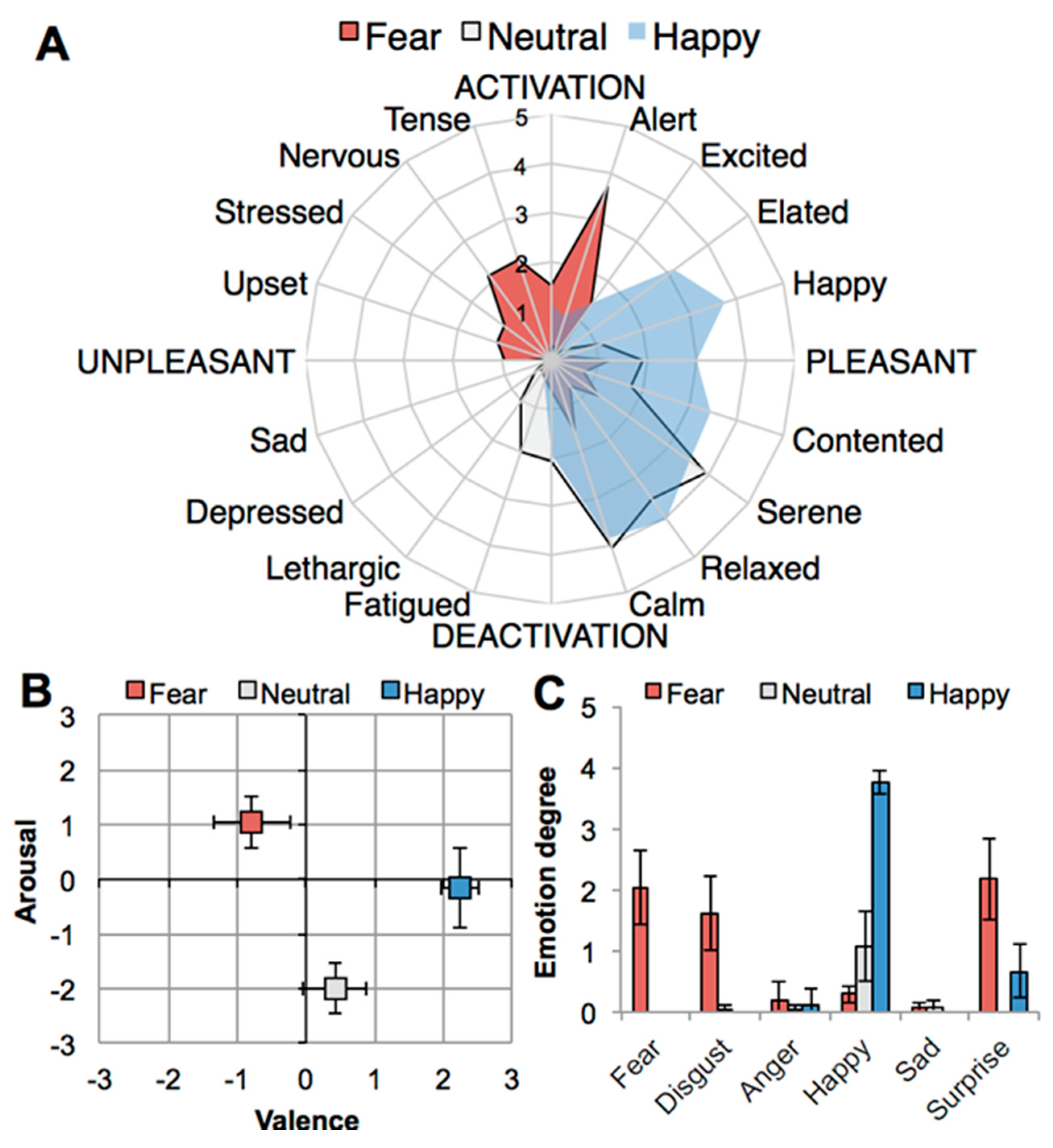
2.1. Emotion Manipulation
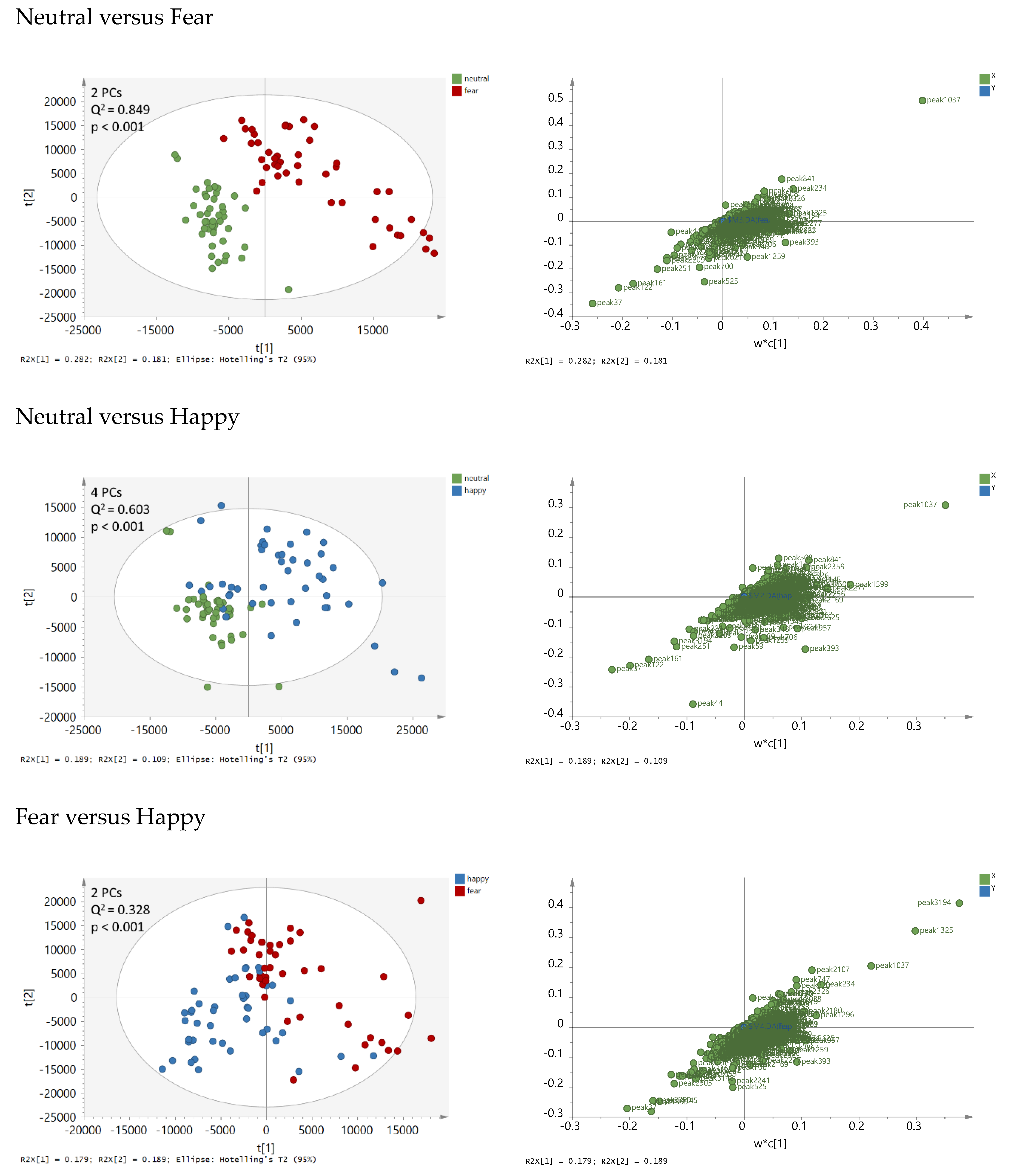
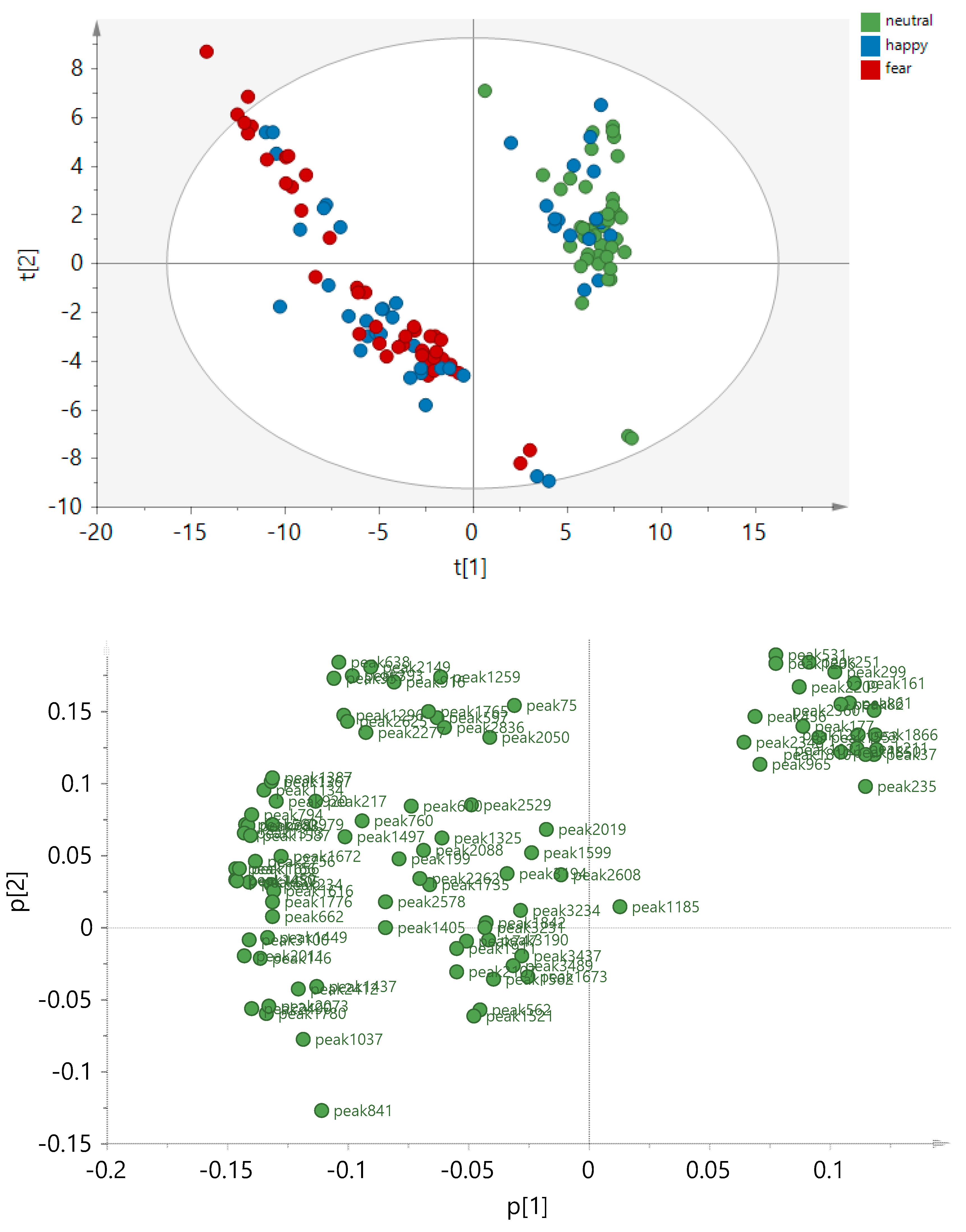
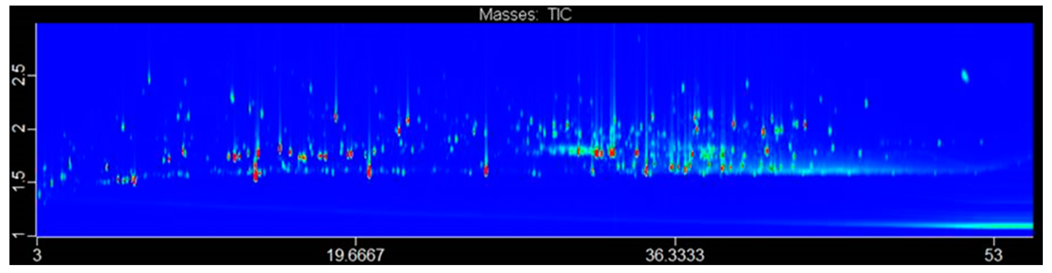
2.2. Chemical Analyses
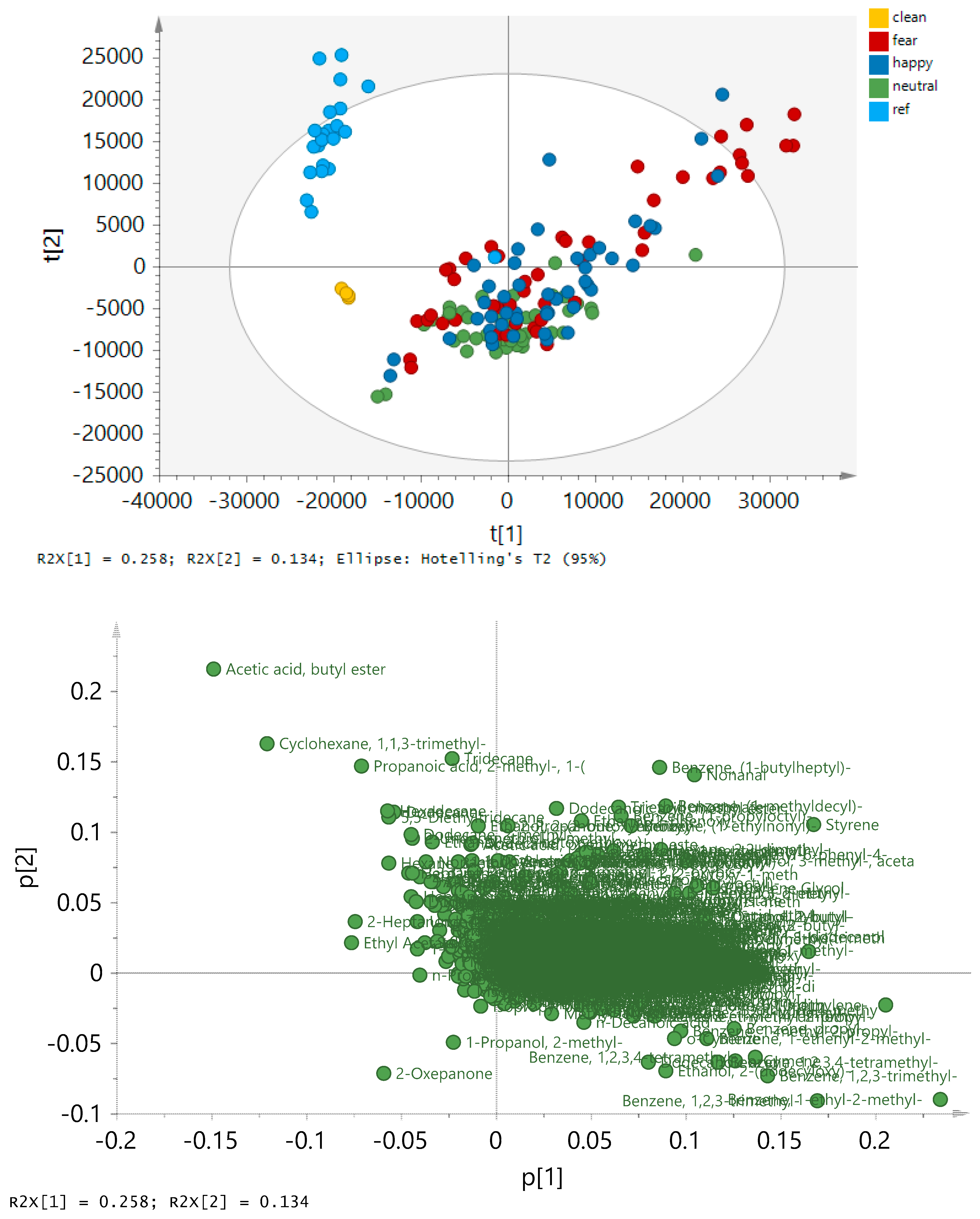
2.3. Exploring the Pattern of Bipolarity
3. Discussion
4. Materials and Methods
4.1. Emotion Induction and Sweat Collection from Donors
4.1.1. Emotion Induction
4.1.2. Manipulation Check
4.1.3. Sweat Donation and Storage
4.2. Sweat Analysis Procedure with GC×GC-TOFMS
4.2.1. Instrumentation
4.2.2. Sample Preparation/Extraction
4.2.3. Thermal Desorption (TD) – GC×GC TOF MS
4.2.4. Data Processing
4.3. Ethics Statement
Supplementary Materials
Author Contributions
Funding
Acknowledgments
Conflicts of Interest
Appendix A. Additional Data Figures and Tables


| Peak | RT Dim 1 | RT Dim 2 | Mass | Discrimination | Up or Down |
|---|---|---|---|---|---|
| 37 | 213.065 | 1.50373 | 43 | F H vs N | D |
| 61 | 252.986 | 1.54448 | 87 | F H vs N | D |
| 75 | 266.896 | 1.69866 | 84 | F H vs N | D |
| 82 | 278.881 | 1.52216 | 87 | F H vs N | D |
| 94 | 290.867 | 1.5497 | 87 | F H vs N | D |
| 122 | 311.842 | 1.70207 | 61 | F H vs N | D |
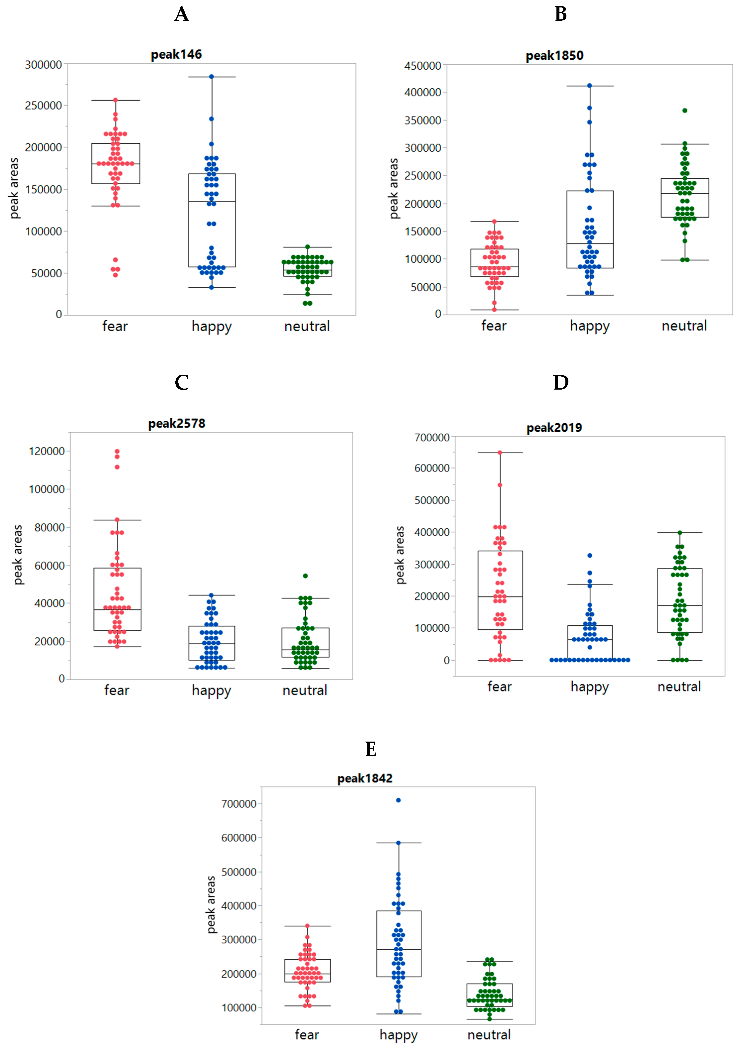
| 146 | 347.798 | 2.07133 | 69 | F H vs N | U |
| 161 | 368.059 | 1.68569 | 59 | F H vs N | D |
| 177 | 381.986 | 2.01085 | 59 | F H vs N | D |
| 199 | 410.852 | 1.84624 | 45 | F H vs N | U |
| 211 | 422.849 | 2.59792 | 43 | F H vs N | D |
| 221 | 431.698 | 2.17416 | 55 | F H vs N | U |
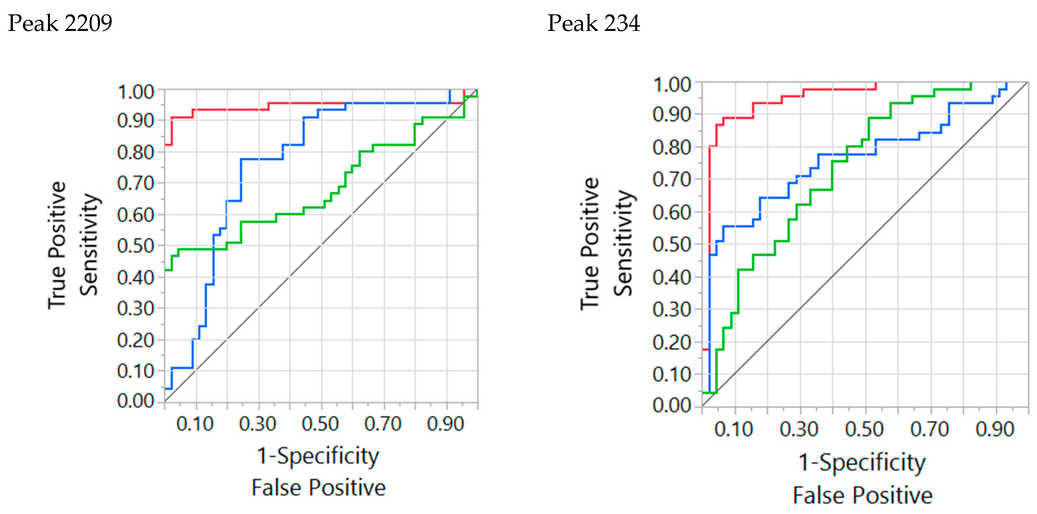
| 234 | 446.54 | 1.94374 | 56 | F H vs N | U |
| 235 | 445.611 | 2.1115 | 45 | F H vs N | D |
| 251 | 470.651 | 1.85195 | 43 | F H vs N | D |
| 299 | 536.554 | 1.81135 | 45 | F H vs N | D |
| 456 | 713.831 | 1.96898 | 61 | F H vs N | D |
| 505 | 773.287 | 2.35098 | 83 | F H vs N | U |
| 531 | 794.262 | 2.88303 | 96 | F H vs N | D |
| 560 | 824.226 | 1.74228 | 57 | F H vs N | U |
| 562 | 823.532 | 1.91573 | 103 | H vs F N | U |
| 638 | 878.161 | 2.06622 | 57 | F H vs N | U |
| 662 | 896.75 | 2.4186 | 81 | F H vs N | U |
| 747 | 967.754 | 2.2181 | 146 | F H vs N | U |
| 760 | 979.795 | 2.2298 | 91 | H vs F N | U |
| 783 | 1001.01 | 0.424779 | 85 | F H vs N | U |
| 794 | 1007.01 | 2.33448 | 70 | F H vs N | U |
| 799 | 1010 | 2.30056 | 99 | F H vs N | U |
| 841 | 1038.33 | 2.20129 | 59 | F H vs N | U |
| 916 | 1084.9 | 1.57542 | 93 | H vs F N | D |
| 920 | 1084.97 | 1.65668 | 81 | F H vs N | U |
| 957 | 1111.88 | 2.04592 | 57 | F H vs N | U |
| 965 | 1118.6 | 1.60533 | 267 | F H vs N | D |
| 979 | 1123.87 | 2.38479 | 81 | F H vs N | U |
| 1021 | 1146.78 | 2.91127 | 87 | F H vs N | D |
| 1037 | 1150.08 | 2.73321 | 99 | F H vs N | U |
| 1134 | 1225.92 | 0.285066 | 85 | F H vs N | U |
| 1166 | 1240.73 | 2.2519 | 113 | F H vs N | U |
| 1185 | 1252.26 | 1.75714 | 207 | H vs F N | U |
| 1206 | 1263.01 | 2.21667 | 101 | F H vs N | D |
| 1296 | 1336.58 | 2.01166 | 57 | F H vs N | U |
| 1313 | 1354.66 | 2.32802 | 81 | F H vs N | U |
| 1367 | 1411.52 | 1.83798 | 59 | F H vs N | U |
| 1387 | 1422.39 | 1.84604 | 59 | F H vs N | U |
| 1405 | 1433.16 | 0.157468 | 113 | H vs F N | U |
| 1437 | 1458.51 | 1.54951 | 163 | F H vs N | U |
| 1449 | 1462.46 | 1.9767 | 58 | F H vs N | U |
| 1450 | 1462.46 | 2.1945 | 127 | F H vs N | U |
| 1457 | 1465.46 | 2.42029 | 131 | F H vs N | U |
| 1497 | 1507.46 | 2.15058 | 59 | H vs F N | U |
| 1521 | 1525.41 | 1.82177 | 207 | H vs F N | U |
| 1553 | 1549.82 | 2.17105 | 59 | F H vs N | D |
| 1562 | 1555.15 | 1.69778 | 281 | H vs F N | U |
| 1587 | 1570.33 | 2.26863 | 81 | F H vs N | U |
| 1599 | 1581.97 | 1.54985 | 73 | H vs F N | U |
| 1616 | 1591.93 | 1.74071 | 59 | F H vs N | U |
| 1656 | 1628.35 | 0.0582741 | 84 | F H vs N | U |
| 1672 | 1639.32 | 1.84592 | 59 | F H vs N | U |
| 1673 | 1638.78 | 2.08221 | 133 | H vs F N | U |
| 1735 | 1687.01 | 1.5716 | 71 | F vs H N | U |
| 1765 | 1711.21 | 1.71539 | 69 | F vs H N | U |
| 1776 | 1717.15 | 1.82356 | 59 | F H vs N | U |
| 1780 | 1723.15 | 1.93293 | 114 | F H vs N | U |
| 1810 | 1741.73 | 2.28162 | 59 | F H vs N | D |
| 1842 | 1762.1 | 1.84815 | 109 | H vs F N | U |
| 1850 | 1767.88 | 2.30028 | 87 | F H vs N | D |
| 1866 | 1777.23 | 2.70362 | 87 | F H vs N | D |
| 1911 | 1804.52 | 1.54262 | 57 | H vs F N | U |
| 2011 | 1848.74 | 1.93918 | 95 | F H vs N | U |
| 2019 | 1848.07 | 1.73778 | 97 | H vs F N | D |
| 2050 | 1867.03 | 1.65334 | 92 | H vs F N | U |
| 2073 | 1875.98 | 2.19588 | 177 | F H vs N | U |
| 2088 | 1884.55 | 1.7368 | 70 | F vs H N | U |
| 2107 | 1893.49 | 1.5439 | 70 | F vs H N | U |
| 2127 | 1902.93 | 1.91097 | 72 | F H vs N | U |
| 2149 | 1913.33 | 1.96941 | 58 | H vs F N | U |
| 2209 | 1944.88 | 1.68335 | 191 | F H vs N | D |
| 2262 | 1974.91 | 1.79818 | 59 | H vs F N | U |
| 2277 | 1980.84 | 1.72275 | 57 | F H vs N | U |
| 2348 | 2013.6 | 2.31272 | 87 | F H vs N | D |
| 2360 | 2022.79 | 2.48686 | 100 | F H vs N | D |
| 2412 | 2046.83 | 1.84665 | 113 | F H vs N | U |
| 2490 | 2091.72 | 1.88072 | 114 | F H vs N | U |
| 2529 | 2112.93 | 1.62908 | 119 | H vs F N | D |
| 2578 | 2139.68 | 1.87183 | 150 | F vs H N | U |
| 2608 | 2156.88 | 1.76811 | 70 | H vs F N | D |
| 2625 | 2165.99 | 1.58243 | 91 | F H vs N | U |
| 2756 | 2220.55 | 1.86757 | 58 | F H vs N | U |
| 3100 | 2391.31 | 2.21692 | 219 | F H vs N | U |
| 3190 | 2457.32 | 1.60417 | 151 | H vs F N | U |
| 3231 | 2493.19 | 1.84005 | 69 | F vs H N | U |
| 3234 | 2496.29 | 1.60178 | 151 | H vs F N | U |
| 3437 | 2739.03 | 1.59881 | 151 | H vs F N | U |
| 3489 | 2830.62 | 1.62092 | 149 | H vs F N | U |
References
- De Groot, J.H.B.; Smeets, M.A.M.; Rowson, M.J.; Bulsing, P.J.; Blonk, C.G.; Wilkinson, J.E.; Semin, G.R. A sniff of happiness. Psychol. Sci. 2015, 26, 684–700. [Google Scholar] [CrossRef] [PubMed]
- Pause, B.M. Processing of body odor signals by the human brain. Chemosens. Percept. 2012, 5, 55–63. [Google Scholar] [CrossRef] [PubMed] [Green Version]
- Semin, G.R.; de Groot, J.H.B. The chemical bases of human sociality. Trends Cogn. Sci. 2013, 17, 427–429. [Google Scholar] [CrossRef] [PubMed]
- Olsson, M.J.; Lundström, J.N.; Kimball, B.A.; Gordon, A.R.; Karshikoff, B.; Hosseini, N.; Sorjonen, K.; Olgart Höglund, C.; Solares, C.; Soop, A.; et al. The scent of disease. Psychol. Sci. 2014, 25, 817–823. [Google Scholar] [CrossRef] [PubMed]
- De Groot, J.H.B.; Smeets, M.A.M. Human fear chemosignaling: Evidence from a meta-analysis. Chem. Senses 2017, 42, 663–673. [Google Scholar] [CrossRef]
- Laidre, M.E.; Johnstone, R.A. Animal signals. Curr. Biol. 2013, 23, R829–R833. [Google Scholar] [CrossRef] [Green Version]
- Chen, D.; Haviland-Jones, J. Human olfactory communication of emotion. Percept. Mot. Skills 2000, 91, 771–781. [Google Scholar] [CrossRef]
- De Groot, J.H.B.; Semin, G.R.; Smeets, M.A.M. Chemical communication of fear: A case of male-female asymmetry. J. Exp. Psychol. Gen. 2014, 143, 1515–1525. [Google Scholar] [CrossRef]
- Mutic, S.; Parma, V.; Brünner, Y.F.; Freiherr, J. You smell dangerous: Communicating fight responses through human chemosignals of aggression. Chem. Senses 2016, 41, 35–43. [Google Scholar] [CrossRef] [Green Version]
- Zhou, W.; Chen, D. Fear-related chemosignals modulate recognition of fear in ambiguous facial expressions. Psychol. Sci. 2009, 20, 177–183. [Google Scholar] [CrossRef]
- Bensafi, M.; Brown, W.M.; Tsutsui, T.; Mainland, J.D.; Johnson, B.N.; Bremner, E.A.; Young, N.; Mauss, I.; Ray, B.; Gross, J.; et al. Sex-steroid derived compounds induce sex-specific effects on autonomic nervous system function in humans. Behav. Neurosci. 2003, 117, 1125–1134. [Google Scholar] [CrossRef] [PubMed]
- Parma, V.; Tirindelli, R.; Bisazza, A.; Massaccesi, S.; Castiello, U. Subliminally perceived odours modulate female intrasexual competition: An eye movement study. PLoS ONE 2012, 7, e30645. [Google Scholar] [CrossRef] [PubMed]
- Martins, Y.; Preti, G.; Crabtree, C.R.; Runyan, T.; Vainius, A.A.; Wysocki, C.J. Preference for human body odors is influenced by gender and sexual orientation. Psychol. Sci. 2005, 16, 694–701. [Google Scholar] [CrossRef] [PubMed]
- Lübke, K.T.; Hoenen, M.; Pause, B.M. Differential processing of social chemosignals obtained from potential partners in regards to gender and sexual orientation. Behav. Brain Res. 2012, 228, 375–387. [Google Scholar] [CrossRef] [PubMed]
- Gelstein, S.; Yeshurun, Y.; Rozenkrantz, L.; Shushan, S.; Frumin, I.; Roth, Y.; Sobel, N. Human tears contain a chemosignal. Science 2011, 331, 226–231. [Google Scholar] [CrossRef] [PubMed] [Green Version]
- Porter, R.H.; Schaal, B. Olfaction and development of social preferences in neonatal organisms. In Handbook of Olfaction and Gustation; Doty, R.L., Ed.; Marcel Dekker: New York, NY, USA, 1995; pp. 299–321. [Google Scholar]
- Havlicek, J.; Roberts, S.C.; Flegr, J. Women’s preference for dominant male odour: Effects of menstrual cycle and relationship status. Biol. Lett. 2005, 1, 256–259. [Google Scholar] [CrossRef] [Green Version]
- McClintock, M.K. Menstrual Synchrony and Suppression. Nature 1971, 229, 244–245. [Google Scholar] [CrossRef]
- Zhengwei, Y.; Schank, J.C. Women do not synchronize their menstrual cycles. Hum. Nat. 2006, 17, 433–447. [Google Scholar]
- Ziomkiewicz, A. Menstrual synchrony: Fact or artifact? Hum. Nat. 2006, 17, 419–432. [Google Scholar] [CrossRef]
- Sorokowska, A.; Sorokowski, P.; Szmajke, A. Does personality smell? Accuracy of personality assessments based on body odour. Eur. J. Pers. 2012, 26, 496–503. [Google Scholar] [CrossRef]
- Wyatt, T.D. The search for human pheromones: The lost decades and the necessity of returning to first principles. Proc. R. Soc. B Biol. Sci. 2015, 282, 20142994. [Google Scholar] [CrossRef] [PubMed] [Green Version]
- Doty, R.L. The Great Pheromone Myth; Johns Hopkins University Press: Baltimore, MD, USA, 2010. [Google Scholar]
- Chen, D.; Katdare, A.; Lucas, N. Chemosignals of fear enhance cognitive performance in humans. Chem. Senses 2006, 31, 415–423. [Google Scholar] [CrossRef] [PubMed] [Green Version]
- De Groot, J.H.B.; Smeets, M.A.M.; Kaldewaij, A.; Duijndam, M.J.A.; Semin, G.R. Chemosignals communicate human emotions. Psychol. Sci. 2012, 23, 1417–1424. [Google Scholar] [CrossRef] [PubMed]
- Kamiloglu, R.G.; Smeets, M.A.M.; de Groot, J.H.B.; Semin, G.R. Fear odor facilitates the detection of fear expressions over other negative expressions. Chem. Senses 2018, 43, 419–426. [Google Scholar] [CrossRef] [PubMed]
- De Groot, J.H.B.; Semin, G.R.; Smeets, M.A.M. I can see, hear, and smell your fear: Comparing olfactory and audiovisual media in fear communication. J. Exp. Psychol. Gen. 2014, 143, 825–834. [Google Scholar] [CrossRef] [PubMed]
- De Groot, J.H.B.; van Houtum, L.A.E.M.; Gortemaker, I.; Ye, Y.; Chen, W.; Zhou, W.; Smeets, M.A.M. Beyond the west: Chemosignaling of emotions transcends ethno-cultural boundaries. Psychoneuroendocrinology 2018, 98, 177–185. [Google Scholar] [CrossRef] [PubMed]
- Dalton, P.; Mauté, C.; Jaén, C.; Wilson, T. Chemosignals of stress influence social judgments. PLoS ONE 2013, 8, e77144. [Google Scholar] [CrossRef] [Green Version]
- Singh, P.B.; Young, A.; Lind, S.; Leegaard, M.C.; Capuozzo, A.; Parma, V. Smelling anxiety chemosignals impairs clinical performance of dental students. Chem. Senses 2018, 43, 411–417. [Google Scholar] [CrossRef] [Green Version]
- Adolph, D.; Meister, L.; Pause, B.M. Context counts! Social anxiety modulates the processing of fearful faces in the context of chemosensory anxiety signals. Front. Hum. Neurosci. 2013, 7, 1–17. [Google Scholar] [CrossRef] [Green Version]
- Pause, B.M.; Lübke, K.; Laudien, J.H.; Ferstl, R. Intensified neuronal investment in the processing of chemosensory anxiety signals in non-socially anxious and socially anxious individuals. PLoS ONE 2010, 5, e10342. [Google Scholar] [CrossRef] [Green Version]
- Mujica-Parodi, L.R.; Strey, H.H.; Frederick, B.; Savoy, R.; Cox, D.; Botanov, Y.; Tolkunov, D.; Rubin, D.; Weber, J. Chemosensory cues to conspecific emotional stress activate amygdala in humans. PLoS ONE 2009, 4, e6415. [Google Scholar] [CrossRef] [PubMed]
- Maier, A.; Scheele, D.; Spengler, F.B.; Menba, T.; Mohr, F.; Güntürkün, O.; Stoffel-Wagner, B.; Kinfe, T.M.; Maier, W.; Khalsa, S.S.; et al. Oxytocin reduces a chemosensory-induced stress bias in social perception. Neuropsychopharmacol. 2019, 44, 281–288. [Google Scholar] [CrossRef] [PubMed]
- Prehn-Kristensen, A.; Wiesner, C.; Bergmann, T.O.; Wolff, S.; Jansen, O.; Mehdorn, H.M.; Ferstl, R.; Pause, B.M. Induction of empathy by the smell of anxiety. PLoS ONE 2009, 4, e5987. [Google Scholar] [CrossRef] [PubMed] [Green Version]
- De Groot, J.H.B.; Semin, G.R.; Smeets, M.A.M. On the communicative function of body odors: A theoretical integration and review. Perspect. Psychol. Sci. 2017, 12, 306–324. [Google Scholar] [CrossRef] [PubMed]
- Goyert, H.F.; Frank, M.E.; Gent, J.F.; Hettinger, T.P. Characteristic component odors emerge from mixtures after selective adaptation. Brain Res. Bull. 2007, 72, 1–9. [Google Scholar] [CrossRef] [Green Version]
- Wysocki, C.J.; Preti, G. Facts, fallacies, fears, and frustrations with human pheromones. Anat. Rec. Part A Discov. Mol. Cell. Evol. Biol. 2004, 281, 1201–1211. [Google Scholar] [CrossRef]
- Dormont, L.; Bessière, J.M.; Cohuet, A. Human skin volatiles: A review. J. Chem. Ecol. 2013, 39, 569–578. [Google Scholar] [CrossRef]
- De Lacy Costello, B.; Amann, A.; Al-Kateb, H.; Flynn, C.; Filipiak, W.; Khalid, T.; Osborne, D.; Ratcliffe, N.M. A review of the volatiles from the healthy human body. J. Breath Res. 2014, 8, 014001. [Google Scholar] [CrossRef]
- Fuller, R.G.; Sheehy-Skeffington, A. Effects of group laughter on responses to humourous material, a replication and extension. Psychol. Rep. 1974, 35, 531–534. [Google Scholar] [CrossRef]
- Devereux, P.G.; Ginsburg, G.P. Sociality effects on the production of laughter. J. Gen. Psychol. 2001, 128, 227–240. [Google Scholar] [CrossRef]
- Provine, R.R. Contagious laughter: Laughter is a sufficient stimulus for laughs and smiles. Bull. Psychon. Soc. 1992, 30, 1–4. [Google Scholar] [CrossRef]
- Gervais, M.; Wilson, D.S. The evolution and functions of laughter and humor: A synthetic approach. Q. Rev. Biol. 2019, 80, 395–430. [Google Scholar] [CrossRef] [PubMed] [Green Version]
- Rottenberg, J.; Ray, R.D.; Gross, J.J. Emotion elicitation using films. In Handbook of Emotion Elicitation and Assessment; Coan, J.A., Allen, J.J.B., Eds.; Oxford University Press: Oxford, UK, 2007; pp. 9–28. [Google Scholar]
- Russell, J.A. A circumplex model of affect. J. Pers. Soc. Psychol. 1980, 39, 1161–1178. [Google Scholar] [CrossRef]
- Russell, J.A.; Weiss, A.; Mendelsohn, G.A. Affect grid: A single-item scale of pleasure and arousal. J. Pers. Soc. Psychol. 1989, 57, 493–502. [Google Scholar] [CrossRef]
- Williams, J.; Stönner, C.; Wicker, J.; Krauter, N.; Derstroff, B.; Bourtsoukidis, E.; Klüpfel, T.; Kramer, S. Cinema audiences reproducibly vary the chemical composition of air during films, by broadcasting scene specific emissions on breath. Sci. Rep. 2016, 6, 25464. [Google Scholar] [CrossRef] [PubMed] [Green Version]
- Preti, G.; Dalton, P.; Maute, C. Analytical identification of stress odors from human breath. HDIAC J. 2019, 6, 10–15. [Google Scholar]
- Zeng, X.; Leyden, J.J.; Lawley, H.J.; Sawano, K.; Nohara, I.; Preti, G. Analysis of characteristic odors from human male axillae. J. Chem. Ecol. 1991, 17, 1469–1492. [Google Scholar] [CrossRef]
- Pandey, S.K.; Kim, K.H. Human body-odor components and their determination. Trends Anal. Chem. 2011, 30, 784–796. [Google Scholar] [CrossRef]
- Shimomura, Y.; Kitaura, Y. Physiological and pathological roles of branched-chain amino acids in the regulation of protein and energy metabolism and neurological functions. Pharmacol. Res. 2018, 133, 215–217. [Google Scholar] [CrossRef]
- Hagenfeldt, L.; Wahren, J. Human Forearm Muscle Metabolism during Exercise III Uptake, release and oxidation of β-hydroxybutyrate and observations on the β-hydroxybutyrate/acetoacetate ratio. Scand. J. Clin. Lab. Invest. 1968, 21, 314–320. [Google Scholar] [CrossRef]
- De Groot, J.H.B.; Smeets, M.A.M.; Semin, G.R. Rapid stress drives chemical transfer of fear from sender to receiver. PLoS ONE 2015, 10, e0118211. [Google Scholar] [CrossRef] [PubMed]
- De Groot, J.H.B.; Kirk, P.A.; Gottfried, J.A. Encoding fear intensity in human sweat. Philos. Trans. R. Soc. B Biol. Sci. 2020. [Google Scholar] [CrossRef]
- De Groot, J.H.B.; Kirk, P.A.; Gottfried, J.A. Titrating the smell of fear: Dose-invariant responses of human chemosignals on behavior, physiology, and the brain. Prep.
- Lenochova, P.; Roberts, S.C.; Havlicek, J. Methods of human body odor sampling: The effect of freezing. Chem. Senses 2009, 34, 127–138. [Google Scholar] [CrossRef] [PubMed] [Green Version]
- Stevenson, R.J. An initial evaluation of the functions of human olfaction. Chem. Senses 2010, 35, 3–20. [Google Scholar] [CrossRef] [PubMed] [Green Version]
- McGann, J.P. Poor human olfaction is a 19th-century myth. Science 2017, 356, eaam7263. [Google Scholar] [CrossRef] [Green Version]
- Schaefer, A.; Nils, F.; Sanchez, X.; Philippot, P. Assessing the effectiveness of a large database of emotion-eliciting films: A new tool for emotion researchers. Cogn. Emot. 2010, 24, 1153–1172. [Google Scholar] [CrossRef]
- Larsen, J.T.; McGraw, A.P.; Cacioppo, J.T. Can people feel happy and sad at the same time? J. Pers. Soc. Psychol. 2001, 81, 684–696. [Google Scholar] [CrossRef]
- Harker, M.; Carvell, A.-M.; Marti, V.P.J.; Riazanskaia, S.; Kelso, H.; Taylor, D.; Grimshaw, S.; Arnold, D.S.; Zillmer, R.; Shaw, J.; et al. Functional characterisation of a SNP in the ABCC11 allele—Effects on axillary skin metabolism, odour generation and associated behaviours. J. Dermatol. Sci. 2014, 73, 23–30. [Google Scholar] [CrossRef]
- Van den Berg, R.A.; Hoefsloot, H.C.; Westerhuis, J.A.; Smilde, A.K.; van der Werf, M.J. Centering, scaling, and transformations: Improving the biological information content of metabolomics data. BMC Genom. 2006, 7, 142. [Google Scholar] [CrossRef] [Green Version]
- Van Velzen, E.J.J.; Westerhuis, J.A.; van Duynhoven, J.P.M.; van Dorsten, F.A.; Hoefsloot, H.C.J.; Jacobs, D.M.; Smit, S.; Draijer, R.; Kroner, C.I.; Smilde, A.K. Multilevel data analysis of a crossover designed human nutritional intervention study. J. Proteome Res. 2008, 7, 4483–4491. [Google Scholar] [CrossRef] [PubMed]
- Association, W.M. World Medical Association Declaration of Helsinki: Ethical Principles for Medical Research Involving Human Subjects. JAMA 2013, 310, 2191–2194. [Google Scholar]


| Feeling | Friedman Test | Comparison Condition (Intended Emotions) | Order | ||
|---|---|---|---|---|---|
| Fear vs. Happy | Fear vs. Neutral | Happy vs. Neutral | |||
| Target State | |||||
| Fear | c2 = 38.00, p < 0.001 | Z = 3.9, p < 0.001 | Z = 3.9, p < 0.001 | Z = 0.0, p > 0.999 | F>H=N |
| Happiness | c2 = 40.77, p < 0.001 | Z = −4.5, p < 0.001 | Z = −2.4, p = 0.017 | Z = 4.2, p < 0.001 | H>N>F |
| Calmness | c2 = 33.11, p < 0.001 | Z = −3.9, p < 0.001 | Z = −4.0, p < 0.001 | Z = −1.7, p = 0.096 | N=H>F |
| Affect Grid | |||||
| Valence | c2 = 34.63, p < 0.001 | Z = −4.2, p < 0.001 | Z = −3.2, p< 0.001 | Z = 3.8, p < 0.001 | H>N>F |
| Arousal | c2 = 31.73, p < 0.001 | Z = 2.6, p < 0.001 | Z = 4.3, p< 0.001 | Z = 3.2, p < 0.001 | F>H>N |
| Other States | |||||
| Tense | c2 = 41.38, p < 0.001 | Z = 4.1, p < 0.001 | Z = 4.1, p < 0.001 | Z = −1.0, p = 0.317 | F>N=H |
| Nervous | c2 = 40.00, p < 0.001 | Z = 4.0, p < 0.001 | Z = 4.0, p < 0.001 | Z = 0.0, p > 0.999 | F>H=N |
| Relaxed | c2 = 39.74, p < 0.001 | Z = −4.3, p < 0.001 | Z = −4.2, p < 0.001 | Z = 1.5, p = 0.137 | H=N>F |
| Alert | c2 = 39.00, p < 0.001 | Z = 4.1, p < 0.001 | Z = 4.2, p < 0.001 | Z = 1.8, p = 0.061 | F>H=N |
| Elated | c2 = 36.90, p < 0.001 | Z = −4.2, p < 0.001 | Z = −1.5, p = 0.141 | Z = 4.0, p < 0.001 | H>N=F |
| Serene | c2 = 30.90, p < 0.001 | Z = −3.8, p < 0.001 | Z = −4.1, p < 0.001 | Z = −1.2, p = 0.213 | N=H>F |
| Content | c2 = 29.54, p < 0.001 | Z = −4.0, p < 0.001 | Z = −2.0, p = 0.050 | Z = 3.6, p < 0.001 | H>N>F |
| Disgust | c2 = 29.39, p < 0.001 | Z = 3.4, p < 0.001 | Z = 3.4, p < 0.001 | Z = −1.0, p = 0.317 | F>N=H |
| Surprised | c2 = 27.49, p < 0.001 | Z = 3.3, p < 0.001 | Z = 3.7, p < 0.001 | Z = 2.6, p = 0.011 | F>H>N |
| Fatigued | c2 = 20.35, p < 0.001 | Z = 0.3, p = 0.752 | Z = −3.5, p < 0.001 | Z = −3.2, p < 0.001 | N > H=F |
| Stressed | c2 = 17.43, p < 0.001 | Z = 2.7, p = 0.007 | Z = 2.7, p = 0.007 | Z = −1.0, p = 0.317 | F>N=H |
| Upset | c2 = 16.29, p < 0.001 | Z = 2.9, p = 0.004 | Z = 2.9, p = 0.004 | Z = −1.4, p = 0.157 | F>N=H |
| Lethargic | c2 = 11.35, p = 0.003 | Z = −0.5, p = 0.593 | Z = −1.9, p = 0.062 | Z = −2.2, p = 0.030 | N>H=F |
| Excited | c2 = 11.15, p = 0.004 | Z = 0.0, p = 0.972 | Z = 3.0, p = 0.002 | Z = 2.9, p = 0.004 | F=H>N |
| Depressed | c2 = 4.00, p = 0.135 | Z = 1.4, p = 0.157 | Z = 0.1, p = 0.916 | Z = 1.8, p = 0.068 | F=H=N |
| Sad | c2 = 2.00, p = 0.368 | Z = 1.0, p = 0.317 | Z = −0.6, p = 0.564 | Z = −1.4, p = 0.157 | F=H=N |
| Angry | c2 = 1.40, p = 0.497 | Z = 0.3, p = 0.785 | Z = 1.4, p = 0.157 | Z = 0.5, p = 0.655 | F=H=N |
| Chemical Class | Condition | |||
|---|---|---|---|---|
| Neutral | Fear | Happy | Subcluster | |
| Esters and 5-rings | High | Low | Low | HF (n = 14) |
| High | HN (n = 8) | |||
| Linear aldehydes/ketones | Low | High | High | HF (n = 14) |
| Low | HN (n = 8) |
| Chemical Class | ||
|---|---|---|
| - | CLASS 1 | CLASS 2 |
| Linear Aldehydes / Ketones / Alcohols | Esters and Some Ring Structures * | |
| 1 | Peak 146: 3-penten-2-one | Peak 37: ethyl acetate |
| 2 | Peak 234: hexanal | Peak 61: 4-methyl-1,3-dioxolane |
| 3 | Peak 505: 2-heptenal | Peak 122: propyl acetate |
| 4 | Peak 560: 1-octen-3-ol | Peak 161: 1-ethoxy-2-propanol |
| 5 | Peak 638: octanal | Peak 251: butyl acetate |
| 6 | Peak 662: 2,4-heptadienal | Peak 531: 2-cyclopenten-1-one, 3-methyl |
| 7 | Peak 794: 2-octenal | Peak 2360: 1,6-dioxacyclododecane-7,12-dione |
| 8 | (Peak 957: nonanal) | |
| 9 | Peak 920: 2-hexylfuran | |
| 10 | Peak 979: octadienal | |
| 11 | Peak 1134: γ-heptyl-lacton | |
| 12 | (Peak 1296: decanal) | |
| 13 | Peak 1313: nonadienal | |
| 14 | Peak 1449: 2-Me-decanal | |
| 15 | Peak 1587: decadienal | |
| 16 | Peak 2127: 3-tridecanone | |
© 2020 by the authors. Licensee MDPI, Basel, Switzerland. This article is an open access article distributed under the terms and conditions of the Creative Commons Attribution (CC BY) license (http://creativecommons.org/licenses/by/4.0/).
Share and Cite
Smeets, M.A.M.; Rosing, E.A.E.; Jacobs, D.M.; van Velzen, E.; Koek, J.H.; Blonk, C.; Gortemaker, I.; Eidhof, M.B.; Markovitch, B.; de Groot, J.; et al. Chemical Fingerprints of Emotional Body Odor. Metabolites 2020, 10, 84. https://doi.org/10.3390/metabo10030084
Smeets MAM, Rosing EAE, Jacobs DM, van Velzen E, Koek JH, Blonk C, Gortemaker I, Eidhof MB, Markovitch B, de Groot J, et al. Chemical Fingerprints of Emotional Body Odor. Metabolites. 2020; 10(3):84. https://doi.org/10.3390/metabo10030084
Chicago/Turabian StyleSmeets, Monique A.M., Egge A.E. Rosing, Doris M. Jacobs, Ewoud van Velzen, Jean H. Koek, Cor Blonk, Ilse Gortemaker, Marloes B. Eidhof, Benyamin Markovitch, Jasper de Groot, and et al. 2020. "Chemical Fingerprints of Emotional Body Odor" Metabolites 10, no. 3: 84. https://doi.org/10.3390/metabo10030084