Article

Assessment of Volatile Aromatic Compounds in Smoke Tainted Cabernet Sauvignon Wines Using a Low-Cost E-Nose and Machine Learning Modelling

by
Vasiliki Summerson
1,
Claudia Gonzalez Viejo
1,
Alexis Pang
1,
Damir D. Torrico
2 and
Sigfredo Fuentes
1,*
1
Digital Agriculture, Food and Wine Group, Faculty of Veterinary and Agricultural Sciences, School of Agriculture and Food, The University of Melbourne, Building 142, Parkville, VIC 3010, Australia
2
Department of Wine, Food and Molecular Biosciences, Faculty of Agriculture and Life Sciences, Lincoln University, Lincoln 7647, Canterbury, New Zealand
*
Author to whom correspondence should be addressed.
Molecules 2021, 26(16), 5108; https://doi.org/10.3390/molecules26165108
Submission received: 23 July 2021 / Revised: 20 August 2021 / Accepted: 21 August 2021 / Published: 23 August 2021
(This article belongs to the Special Issue Smoke Taint in Grapes and Wine)

Abstract

:
Wine aroma is an important quality trait in wine, influenced by its volatile compounds. Many factors can affect the composition and levels (concentration) of volatile aromatic compounds, including the water status of grapevines, canopy management, and the effects of climate change, such as increases in ambient temperature and drought. In this study, a low-cost and portable electronic nose (e-nose) was used to assess wines produced from grapevines exposed to different levels of smoke contamination. Readings from the e-nose were then used as inputs to develop two machine learning models based on artificial neural networks. Results showed that regression Model 1 displayed high accuracy in predicting the levels of volatile aromatic compounds in wine (R = 0.99). On the other hand, Model 2 also had high accuracy in predicting smoke aroma intensity from sensory evaluation (R = 0.97). Descriptive sensory analysis showed high levels of smoke taint aromas in the high-density smoke-exposed wine sample (HS), followed by the high-density smoke exposure with in-canopy misting treatment (HSM). Principal component analysis further showed that the HS treatment was associated with smoke aroma intensity, while results from the matrix showed significant negative correlations (p < 0.05) were observed between ammonia gas (sensor MQ137) and the volatile aromatic compounds octanoic acid, ethyl ester (r = −0.93), decanoic acid, ethyl ester (r = −0.94), and octanoic acid, 3-methylbutyl ester (r = −0.89). The two models developed in this study may offer winemakers a rapid, cost-effective, and non-destructive tool for assessing levels of volatile aromatic compounds and the aroma qualities of wine for decision making.

1. Introduction

Wine aroma is a critical component of wine quality and is determined by the combinations and complex interactions of numerous volatile compounds [1,2,3]. Understanding the aroma character of wine is essential for ensuring quality and consumer acceptance in a competitive market. Hence, identifying the volatile aromatic compounds present in wines can provide valuable information on the sensory attributes of the wine and the viticultural and/or winemaking practices that could be altered to improve the quality [4,5,6] or maintain a certain wine style.
Numerous factors can influence the volatile aromatic compound composition of wines, including environmental conditions, viticultural practices, such as crop-level reduction, and drying of fruit, canopy management, and winemaking practices, such as yeast selection and the use of malolactic bacteria [7,8,9,10]. Furthermore, it has been predicted that the effects of climate change may have profound impacts on the aromatic potential of grapes and hence wine quality [11], particularly the increased risk and incidence of bushfires, resulting in grapevine smoke exposure and smoke taint in wines [12,13,14]. Grapevine exposure to smoke during the critical stages between veraison and harvest has been shown to alter the volatile aromatic composition of grapes and lead to the development of smoke taint in wine, resulting in objectionable smoky characters and reduced wine quality [12,13,14,15,16]. Volatile phenols present in smoke, including guaiacol and 4-methylguaiacol, are responsible for the development of smoke aromas in smoke tainted wines such as burnt wood, burning rubber, medicinal, and smoked meats [13,15,16]. In addition to this, increases in temperature and drought brought on by climate change can also affect the aromatic compounds in grapes and hence wine quality [11,17].
The assessment of the volatile aromatic compound composition of wine typically involves expensive instrumentation such as Gas Chromatography–Mass Spectrometry (GC–MS). However, this form of assessment requires the use of specialised equipment, tedious sample preparation, and trained personnel [18,19,20]. In addition, sensory evaluation using a trained panel is often employed to assess wine quality [5,21]. However, this form of assessment requires the recruitment and training of a large number of participants, which can be expensive and time-consuming, and the results may be subject to bias due to individual variability of the participants, which may affect their taste and smell [5,21,22]. There is, therefore, a need for a rapid, cost-effective method for assessing the volatile aromatic compound and sensory qualities of wine that winemakers can use in the winery [18].
Electronic noses (e-noses) typically consist of an array of gas sensors (e.g., metal oxide semiconductors) coupled with a data processing unit and pattern recognition methods to identify the aroma profiles [12,23,24]. They have been used for numerous applications in the food and beverage industry, including for assessment of geographical origin [23,25], assessing quality, and spoilage [26,27,28], as well as for food safety and adulteration detection [29]. E-noses offer numerous advantages for analysing wine aromatic compounds, including ease of use, rapid results, portability, and non-destructive nature [24,25]. Research by Fuentes et al. [12] found that a low-cost e-nose coupled with machine learning modelling is an effective tool for predicting levels of smoke-derived volatile phenols and their glycoconjugates in smoke-tainted Cabernet Sauvignon wines. Other research by Shim and Lee [30] found a portable and inexpensive e-nose to be effective in classifying French red wines and monitoring wine aging, while research by Han et al. [21] also found a low-cost e-nose and voltammetric tongue effective tools for identifying red wines that differ in geographical origin.
This study explored the use of a low-cost and portable e-nose to assess volatile aromatic compounds and smoke aroma intensity in wines produced from grapes exposed to different densities of smoke exposure with or without in-canopy misting. The e-nose readings were used as inputs for machine learning to develop two artificial neural network (ANN) regression models. Model 1 was constructed using the mean values for the peak areas of the volatile aromatic compounds from GC–MS as targets, while Model 2 was developed using the smoke aroma intensity responses from a trained sensory panel. The two models developed displayed high accuracies in predicting the levels of volatile aromatic compounds and smoke aroma intensity in wine. This can offer winemakers a rapid, cost-effective, and non-destructive tool for assessing the aroma qualities of wine.

2. Results and Discussion

2.1. GC–MS Analysis

Mean values for the peak areas of the volatile aromatic compounds and their standard errors are shown in Table 1. Significant differences (p < 0.05) between different smoke treatments were seen for nonanoic acid, ethyl ester, ethyl 9-decenoate, decanoic acid, ethyl ester, octanoic acid, 3-methylbutyl ester, and dodecanoic acid, ethyl ester. The LS sample showed peaks particularly related to aromatic compounds such as decanoic acid, ethyl ester and dodecanoic acid, ethyl ester. These two compounds are associated with grape, fruity, candy, floral, waxy, oily, and soapy aromas (Table 1). The volatile aromatic compounds observed are fatty acid esters formed during fermentation by yeast, with high levels arising in the LS treatment potentially due to increased fermentation activity. Kennison et al. [15] found that grapevine smoke exposure resulted in increased levels of free amino nitrogen (FAN) in grapes and an increased fermentation rate in grapes exposed to repeated smoke exposure. This increased activity by fermentation yeasts may have resulted in greater levels of fatty acid esters. Furthermore, smoke exposure negatively affects grape ripening, such as sugar accumulation. Previous research also showed that high levels of smoke exposure resulted in increased leaf senescence, which can also impact grape maturation and ripening [15,31]. Therefore, these factors may have reduced the aromatic compound potential of the HS and HSM treatment wines [32,33].

2.2. Smoke Aroma Intensity

Figure 1 shows the means and standard error for smoke aroma intensity according to the different smoke treatments. There were significant differences (p < 0.05) between samples. As expected, the HS treatment had the highest mean response for smoke aroma intensity (11.52), followed by the HSM treatment (7.17), while the C and CM treatments exhibited the lowest mean value (0.76 and 1.24, respectively). This is in line with previous studies showing the development of smoke aromas following grapevine smoke exposure, with repeated exposure resulting in a cumulative effect on the levels of smoke-derived volatile phenols [13,15,16]. Wines produced from grapes exposed to smoke have been shown to contain higher levels of smoke-derived volatile phenols and exhibit greater smoky characteristics, described as burnt rubber, smoked meat, and disinfectant/hospital [15]. Therefore, there is no surprise that the HS exhibited the highest mean value for smoke aroma intensity, while the two control treatments exhibited the lowest.

2.3. Electronic Nose

Figure 2 shows the mean values and standard errors for each gas sensor integrated into the e-nose for each wine sample. Significant differences (p < 0.05) were found between wine samples for all gas sensors in the e-nose. The highest readings for all samples were observed for ethanol gas release (sensor MQ3), with the CM treatment exhibiting the highest mean value (3.97 V) and the LS treatment showing the lowest (3.62 V). The lowest readings for all wine samples were seen for hydrogen sulphide gas (sensor 136), with the CM treatment displaying the highest reading again (0.30 V) and the C treatment exhibiting the lowest reading (0.23 V). Hydrogen sulphide (H2S) is produced naturally during fermentation by yeast and is responsible for negative aromas in wine, such as rotten eggs, sewage, and cooked cabbage, which can develop after the wine has been bottled [36,37,38,39,40]. Therefore, it is necessary for winemakers to know the concentration of H2S in wine and ensure it is kept to a minimum [37]. Readings for the CO2 gas sensor (sensor MG811) are inversed; therefore, lower volts mean a higher concentration. The C treatment showed the lowest reading (1.16 V) and, hence, the highest concentration of CO2, while the HSM, HS, and LS treatments exhibited the highest readings (1.33 V) and, therefore, the lowest CO2 concentration. The CM wines showed the highest mean values for most gases, including ethanol (sensor MQ3), hydrogen (sensor MQ8), and ammonia, alcohol, and benzene (sensor MQ135). As winemaking practices were the same for all the wine samples produced, this may be due to the misting treatment, which may have impacted the grape berries. In particular, misting may have impacted the natural flora present on the grape berries by increasing the humidity surrounding the grape bunch. Therefore, the resulting increase in natural flora may have affected fermentation and the gases produced [41].

2.4. Multivariate Data Analysis

Figure 3 shows the principal component analysis (PCA) with data from the e-nose readings, volatile aromatic compounds, and smoke aroma intensity. Principal component one (PC1) represented 56.1% of the data variability, and principal component two (PC2) accounted for 19.11%, with a total of 75.20% of the data variability. According to the factor loadings (FL), PC1 was primarily represented by octanoic acid, 3-methylbutyl ester (FL = 0.31), hexanoic acid, ethyl ester (FL = 0.28), ethyl 9-decenoate and dodecanoic acid, ethyl ester (FL = 0.27 for each) on the positive side, and gas sensors MQ135 (FL = −0.28), MQ137 (FL = −0.28), and MQ4 (FL = −0.24) on the negative side of the axis. On the other hand, PC2 was mainly represented by MG811 gas sensor (FL = 0.45), smoke aroma intensity (FL = 0.41) and benzene methanol, alpha-methyl-(FL = 0.33) on the positive side of the axis, and MQ7 gas sensor (FL = −0.45), hexanoic acid, ethyl ester (FL = −0.24), and octanoic acid, ethyl ester (FL = −0.14) on the negative side. It can be observed that the HS and LS wine samples were grouped and associated with volatile aromatic compounds, including dodecanoic acid, ethyl ester, decanoic acid, ethyl ester, octanoic acid, 3-methylbutyl ester, and benzene methanol, alpha-methyl-, in line with the GC–MS results. These results coincide with findings from Summerson et al. [42] in smoke tainted Pinot Grigio wines. Furthermore, HS and LS samples were also associated with smoke aroma intensity and carbon dioxide gas (sensor MG811). The HSM treatment was associated with methane (gas sensor MQ4). According to the MQ4 sensor specifications, it has some sensitivity to smoke, explaining its relationship with the HSM treatment.
On the other hand, the CM treatment was associated with ammonia, alcohol, and benzene (sensor MQ135), and ethanol (sensor MQ3), benzene, alcohol, and ammonia (gas sensor 138), and hydrogen sulphide (sensor MQ136), while the C treatment as associated with carbon monoxide (sensor MQ7). The associations found between CM and the gas sensors mentioned are in accordance with results presented by Summerson et al. [42] for control (non-smoked) Pinot Grigio wines with an amelioration activated carbon treatment.
Significant correlations (p < 0.05) between the sensory parameters, e-nose readings, and volatile aroma compounds are displayed in Figure 4. Positive correlations could be seen between ammonia, alcohol, and benzene gas (sensor MQ135) and hydrogen gas (sensor MQ8) (r = 0.92) and benzene, alcohol, and ammonia gases (sensor MQ138; r = 0.90). This correlation between MQ135 and MQ138 was expected as, even though they have different sensitivity, both can detect ammonia [43]. Negative correlations were observed between ammonia gas (sensor MQ137) and octanoic acid, ethyl ester (r = −0.93), decanoic acid, ethyl ester (r = −0.94) and octanoic acid, 3-methylbutyl ester (r = −0.89), as well as between ethanol gas (sensor MQ3) and octanoic acid, 3-methylbutyl ester (r = −0.88), and dodecanoic acid, ethyl ester (r = −0.90).

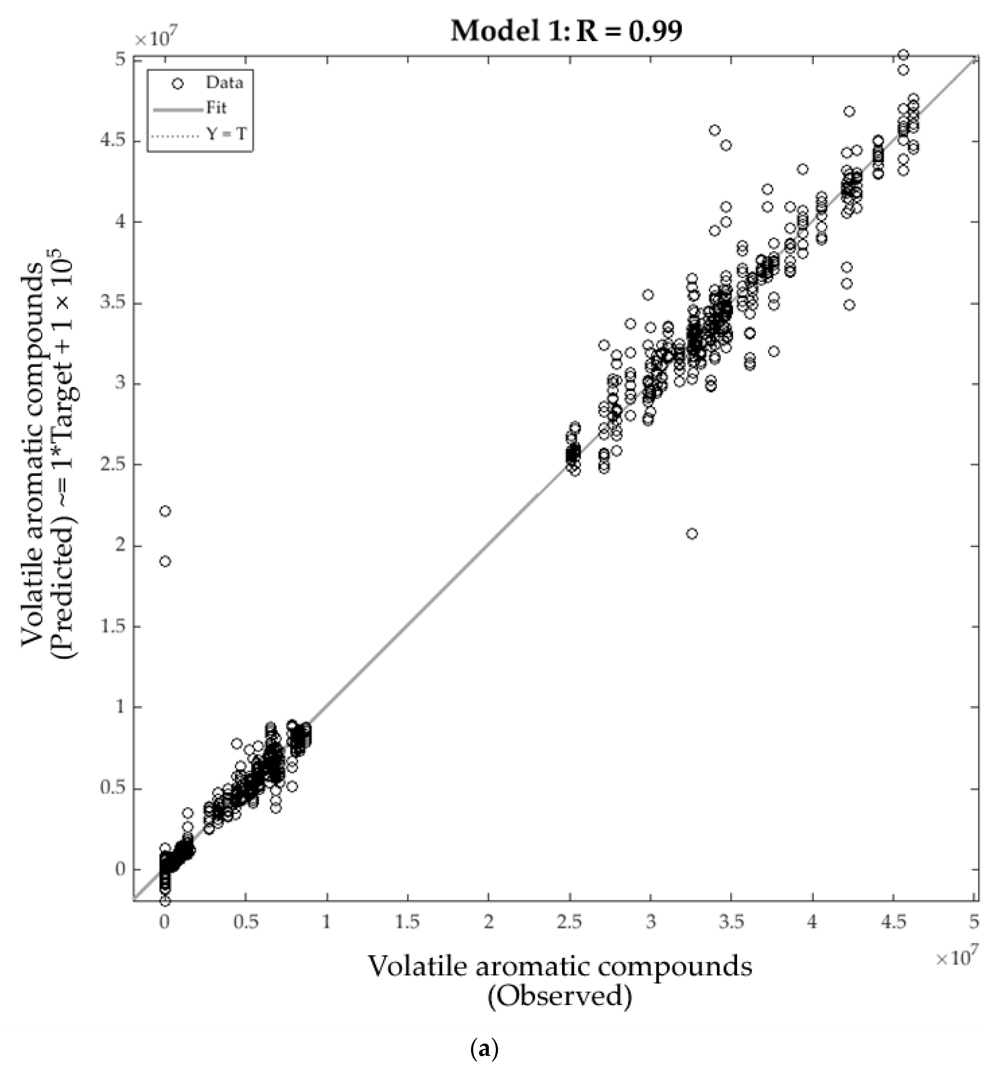
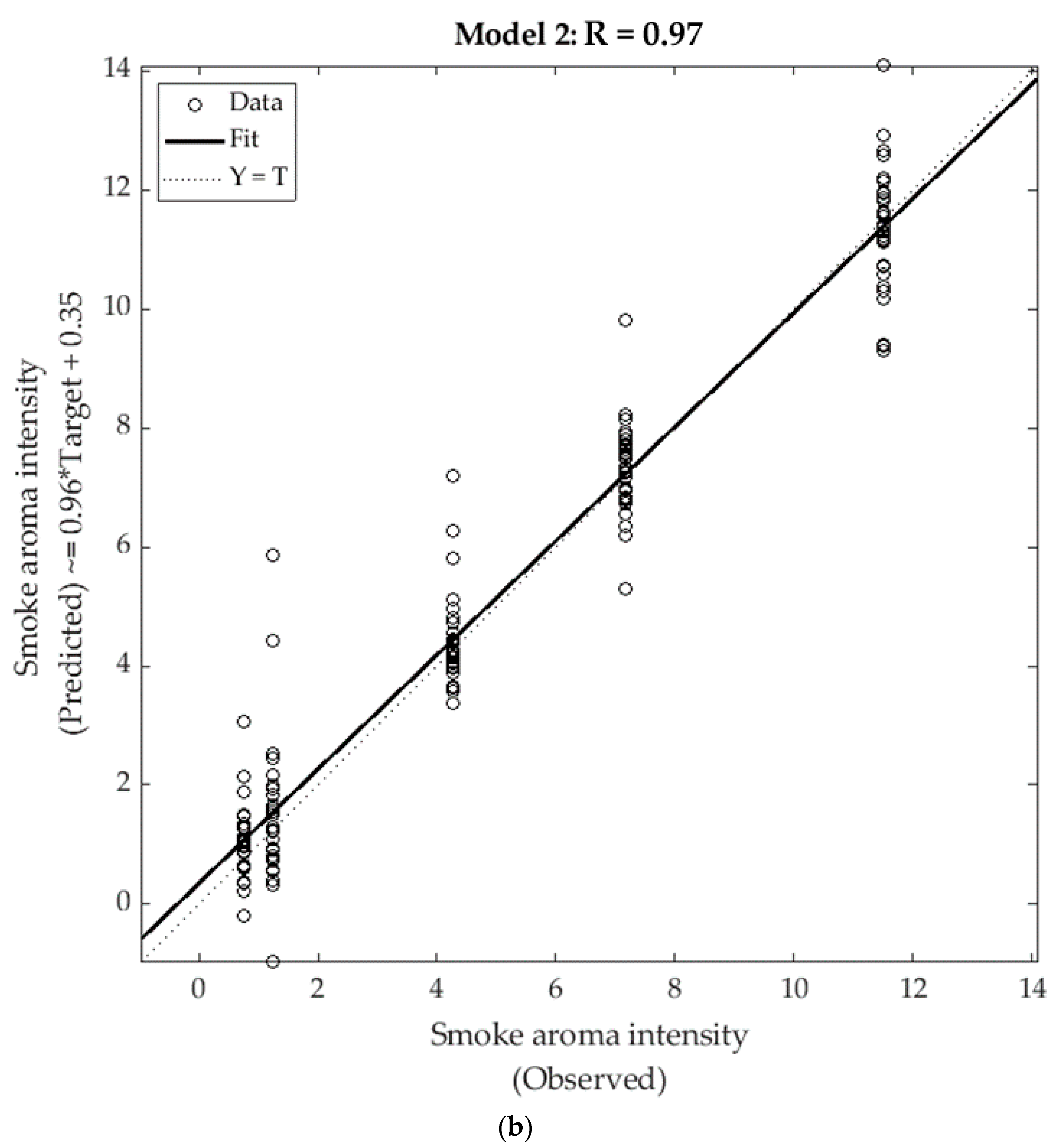
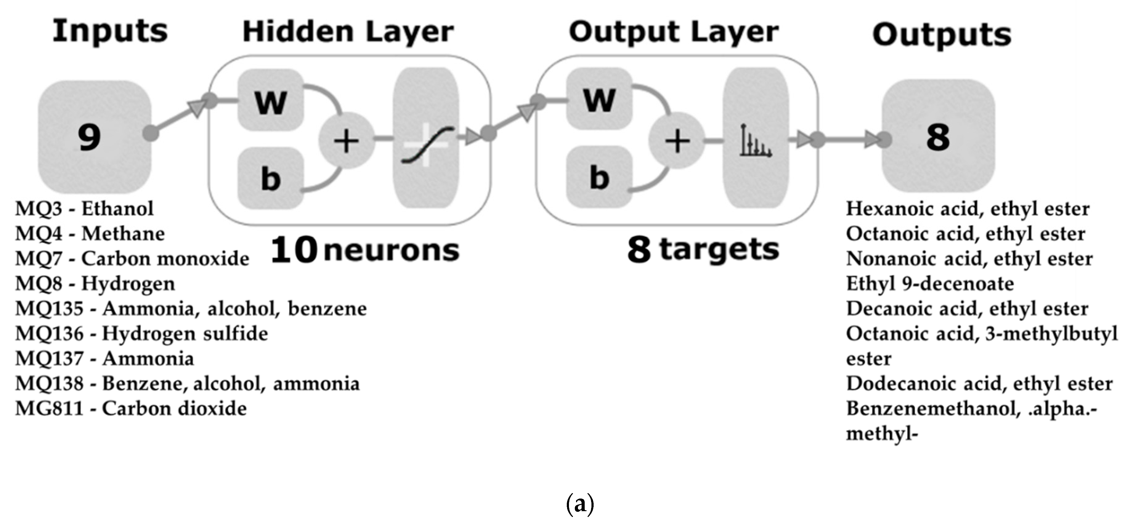
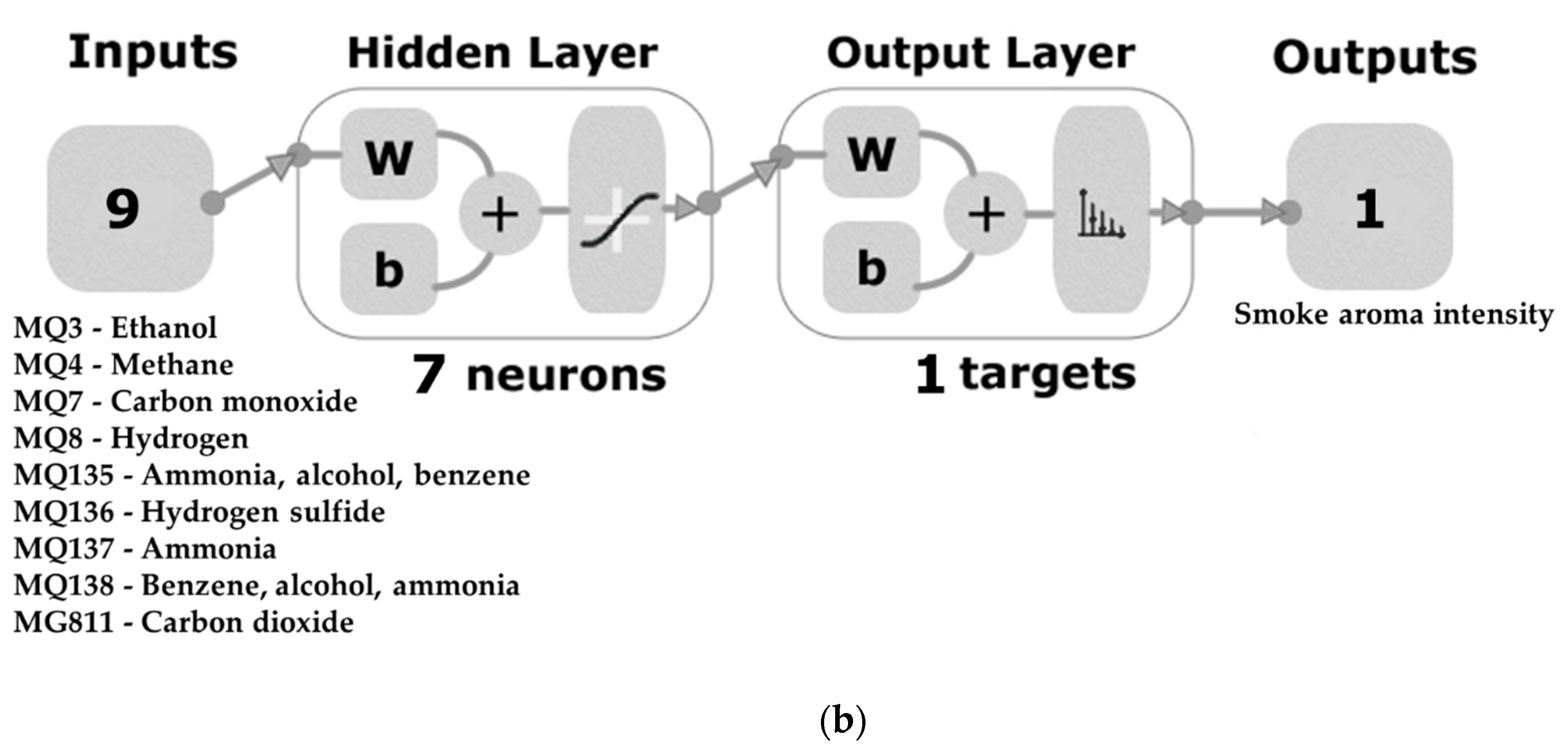
2.5. Machine Learning Modelling

Table 2 shows the statistical data for the artificial neural network (ANN) regression models developed to predict the levels of volatile aromatic compounds (Model 1) and smoke aroma intensities (Model 2) in the wine samples. Model 1 displayed a high overall correlation and determination coefficients (R = 0.99, R2 = 0.98; Figure 5a). Furthermore, there were no signs of over- or underfitting as illustrated by the performance values for the training stage (MSE = 8.39 × 10¹²) being lower than that for the testing stage (MSE = 5.24 × 10¹¹). In addition to this, Model 2 also displayed high overall correlation and determination coefficients (R = 0.97, R2 = 0.94; Figure 5b), with the performance values for the training stage (MSE = 0.42) once again being lower than that for the testing stage (MSE = 2.76).
The ANN regression models developed in this study displayed high accuracy in predicting the levels of volatile aromatic compounds and smoke aroma intensity in wine. This may offer winemakers cost-effective, rapid tools for assessing the aroma and quality of the wine. Due to the learning capacity of ANN, the models may be further fed with more aromatic volatile compounds to improve and enhance their functionality. Furthermore, as the use of an e-nose is non-destructive, repeated measurements are possible. This may be particularly useful for smoke tainted wines as winemakers can assess the aroma potential of wines before and after applying smoke taint amelioration treatments. Summerson et al. [42] used the e-nose coupled with machine learning modelling to assess the effectivity of smoke taint amelioration treatments in Pinot Grigio wines. Furthermore, Fuentes et al. [12] developed an ANN model using e-nose readings as inputs to predict the levels of 7 volatile phenols and 17 glycoconjugates in wine. The use of these models coupled with the two models developed in this study may provide winemakers with tools to accurately assess the quality of smoke tainted wines in near real-time.

3. Materials and Methods

3.1. Smoke Treatments and Winemaking

Field trials describing smoke and misting treatments have been previously reported by Szeto et al. [44] and Summerson et al. [31] and consisted of: (i) a control treatment (C; i.e., no smoke exposure or in-canopy misting); (ii) a control treatment with in-canopy misting (CM); (iii) high-density smoke exposure (HS); (iv) high-density smoke exposure with in-canopy misting (HSM); and (v) a low-density smoke exposure (LS). Smoke treatments were applied at approximately seven days post-veraison by pumping smoke derived from the combustion of barley straw into purpose-built tents for one hour. Misting was applied on the same day as the smoking treatments, and it was achieved using a purpose-built sprinkler system that delivered water at 11 L h−1 and provided a constant supply of fine water droplets (65 µm) to the grape bunch zone [44,45]. The misting sprinkler system was turned on 5 min before the smoking treatment and turned off 15 min after the treatment; this lasted for a total of 2.5 h because the smoke had to be applied in two sessions (one for each half of vines) as not all vines fitted inside the tent used to isolate smoking. Treatments were applied to six adjacent vines, except for the HSM, which was applied to five adjacent vines, with a minimum of one buffer vine separating all treatments. Once grapes reached maturity, they were harvested for winemaking. The wine was produced on a small scale (~5 kg per fermentation, conducted in triplicate per treatment), as previously described [44].

3.2. GC–MS Analysis

Analysis of volatile aromatic compounds was undertaken using a Gas-Chromatograph with a Mass-Selective Detector 5977B (GC-MSD; Agilent Technologies, Inc., Santa Clara, CA, USA) using an HP-5MS column (length 30 m, inner diameter 0.25 mm and film 0.25 µ; Agilent Technologies, Inc., Santa Clara, CA, USA) with helium as the carrier gas (flow rate of 1 mL min−1) and an integrated autosampler system PAL3 (CTC Analytics AG, Zwingen, Switzerland). The assessment was conducted in triplicates for each smoke treatment using 5 mL of wine sample that was placed in a 20 mL vial and then analysed using the headspace method with a solid-phase microextraction (SPME) divinylbenzene–carboxen–polydimethylsiloxane (DVB–CAR–PDMS) 1.1 mm grey fibre (Agilent Technologies, Inc.), with a blank vial used at the start to prevent any carryover effects. Additional details about the method used are described by Gonzalez Viejo et al. [46]. Compounds were identified using the National Institute of Standards and Technology (NIST; National Institute of Standards and Technology, Gaithersburg, MD, USA) library, and only compounds with greater than 80% certainty were used for this study.

3.3. Assessment of Smoke Aroma Intensity

Sensory evaluation investigating the smoke aroma intensity of the wine samples was conducted in the sensory laboratory of the Faculty of Veterinary and Agricultural Sciences (FVAS). The sensory panel consisted of 13 participants (age: 26–46 years; gender: 69% female and 31% male) from the staff and students at the University of Melbourne (UoM; Ethics ID: 1545786.2). Panellists were previously trained using the quantitative descriptive analysis (QDA®) method. The session was undertaken in individual booths equipped with a tablet PC programmed with the Bio-Sensory Application (The University of Melbourne, Parkville, VIC, Australia; [47]), which displayed the questionnaire. All wine samples were assigned a randomly generated 3-digit random code to avoid bias. Participants received 10 mL of each wine sample served at room temperature (~20 °C) in International Standard Wine Tasting Glasses (Bormioli Luigi, Fidenza, Italy). The degree of smoke aroma intensity was rated on a 15-cm intensity scale (absent–intense). Each sample was evaluated independently (monadically), and participants used plain room temperature water and water crackers as palate cleansers.

3.4. Electronic Nose

A low cost, portable e-nose developed by the Digital Agriculture, Food and Wine (DAFW) Group from the FVAS of the UoM and comprised of an array of nine gas sensors with sensitivity to different gases was used to assess the wine samples in triplicates, as previously described [12,43]. The nine sensors and the gases they are sensitive to were: (i) MQ3 = ethanol; (ii) MQ4 = methane; (iii) MQ7 = carbon monoxide; (iv) MQ8 = hydrogen; (v) MQ135 = ammonia, alcohol, and benzene; (vi) MQ136 = hydrogen sulphide; (vii) = MQ137 = ammonia; (viii) MQ138 = benzene, alcohol, and ammonia; and (ix) MG811 = carbon dioxide. Measurements were conducted by pouring 100 mL of wine sample into a 500 mL beaker, stirring the liquid once, and placing the e-nose on top, which fully covered the beaker for approximately 1 min to collect the gas readings. The e-nose has some holes in between the sensors to allow airflow and avoid oversaturation of the gases. The e-nose was calibrated for 20–30 s between samples to prevent carryover effects between sample readings.
Data from the e-nose was acquired using a customised code written in MATLAB® R2020a (MathWorks, Inc., Natick, MA, USA) to identify the stable signals from when the e-nose was placed on the beaker containing the sample until just before it was removed. Following this, the data was automatically divided into 10 subdivisions to extract the average values per sensor, as previously detailed by Gonzalez Viejo et al. [22]. The average values were then used as inputs for machine learning modelling.

3.5. Statistical Analysis and Machine Learning Modelling

Analysis of variance (ANOVA) was performed using Minitab® version 19.2020.1 (Minitab Inc., State College, PA, USA) for the sensory response towards smoke aroma intensity, e-nose readings, and relative peak areas of the volatile compounds identified by GC–MS, with mean comparisons performed using the Fisher’s least significant difference (LSD) post-hoc test at α = 0.05 to assess if there were significant differences between wine samples. Principal component analysis (PCA) was performed for the sensory response, e-nose readings and volatile aromatic compounds using a customised code written in MATLAB® R2020a, while a matrix was also developed using MATLAB® R2020a to assess the significant correlations (p < 0.05) between these parameters.
Machine learning modelling based on ANN was performed to develop the regression models using a customised code written in MATLAB® R2020a that tested 17 different training algorithms, as Gonzalez Viejo et al. [48] described previously. The 10 mean values of each of the e-nose outputs for each replicate of the five smoke treatments were used as inputs to predict levels of: (i) the eight volatile aromatic compounds present in the wine samples (Model 1; Figure 6a), and (ii) the level of smoke aroma intensity (Model 2; Figure 6b). The Bayesian Regularisation algorithm was the best for both models based on the high accuracy and performance observed, with further training performed to develop more accurate ANN models, with no signs of under- or overfitting. Input data were divided randomly, with 80% used for training and 20% used for testing for each model, with performance tested based on mean squared error (MSE). Ten neurons were used for Model 1, while seven were used for Model 2 following a trimming test with 3, 7, and 10 neurons (data not shown).

4. Conclusions

The use of a low-cost, portable electronic nose coupled with machine learning may offer winemakers a more cost-effective and rapid tool for assessing levels of volatile aromatic compounds and the degree of smoke aroma intensity in wine. Furthermore, the non-destructive nature of this form of assessment allows for repeated measurements, allowing winemakers to assess the quality of wine samples before and after the application of smoke-taint amelioration treatments in smoke tainted wines. The ANN regression models may also be used alongside previously developed models that assess the levels of smoke derived volatile phenols and their glycoconjugates and consumer sensory responses towards wine samples for an in-depth quality assessment of smoke-tainted wines.

Author Contributions

Conceptualisation, V.S., C.G.V., and S.F.; data curation, V.S., C.G.V., and S.F.; formal analysis, V.S.; funding acquisition, S.F.; investigation, V.S., and C.G.V.; methodology, V.S., C.G.V., and S.F.; project administration, S.F.; resources, S.F.; software, C.G.V., and S.F.; supervision, D.D.T., A.P., and S.F.; validation, C.G.V., S.F.; visualisation, V.S., C.G.V., D.D.T., A.P., and S.F.; writing—original draft, V.S.; writing—review and editing, V.S., C.G.V., D.D.T., A.P., and S.F. All authors have read and agreed to the published version of the manuscript.

Funding

This research was supported through the Australian Government Research Training Program Scholarship. Colleen Szeto was supported by the Australian Research Council Training Centre for Innovative Wine Production (www.arcwinecentre.org.au) funded as part of the ARC Industrial Transformation Research Program (project no. ICI70100008), with support from Wine Australia and industry partners.

Institutional Review Board Statement

The study was approved by the Human Ethics Advisory Group (HEAG) of The University of Melbourne (Ethics ID: 1545786.2).

Informed Consent Statement

Informed consent was obtained from all subjects involved in the study.

Data Availability Statement

Data and intellectual property belong to The University of Melbourne; any sharing needs to be evaluated and approved by the university.

Acknowledgments

The authors gratefully acknowledge Kerry Wilkinson and Colleen Szeto for the opportunity to collaborate in the field trials and for supplying wine samples for analysis. The authors would like to acknowledge Ranjith R. Unnithan and Bryce Widdicombe from the School of Engineering, Department of Electrical and Electronic Engineering at The University of Melbourne for their collaboration in the electronic nose development.

Conflicts of Interest

The authors declare no conflict of interest.

Sample Availability

Samples of the compounds are not available.

References

  1. Arcari, S.G.; Caliari, V.; Sganzerla, M.; Godoy, H.T. Volatile composition of Merlot red wine and its contribution to the aroma: Optimisation and validation of analytical method. Talanta 2017, 174, 752–766. [Google Scholar] [CrossRef]
  2. Ayestarán, B.; Martínez-Lapuente, L.; Guadalupe, Z.; Canals, C.; Adell, E.; Vilanova, M. Effect of the winemaking process on the volatile composition and aromatic profile of Tempranillo Blanco wines. Food Chem. 2019, 276, 187–194. [Google Scholar] [CrossRef]
  3. Zhao, P.; Qian, Y.; He, F.; Li, H.; Qian, M. Comparative characterisation of aroma compounds in merlot wine by lichrolut-en-based aroma extract dilution analysis and odor activity value. Chemosens. Percept. 2017, 10, 149–160. [Google Scholar] [CrossRef]
  4. McKay, M.; Bauer, F.; Panzeri, V.; Mokwena, L.; Buica, A. Profiling potentially smoke tainted red wines: Volatile phenols and aroma attributes. S. Afr. J. Enol. Vitic. 2019, 40, 1. [Google Scholar]
  5. Sherman, E.; Harbertson, J.F.; Greenwood, D.R.; Villas-Bôas, S.G.; Fiehn, O.; Heymann, H. Reference samples guide variable selection for correlation of wine sensory and volatile profiling data. Food Chem. 2018, 267, 344–354. [Google Scholar] [CrossRef]
  6. Siebert, T.E.; Stamatopoulos, P.; Francis, I.L.; Darriet, P. Sensory-directed characterisation of distinctive aromas of Sauternes and Viognier wines through semi-preparative liquid chromatography and gas chromatography approaches. J. Chromatogr. A 2021, 1637, 461803. [Google Scholar] [CrossRef]
  7. Forde, C.G.; Cox, A.; Williams, E.R.; Boss, P.K. Associations between the sensory attributes and volatile composition of Cabernet Sauvignon wines and the volatile composition of the grapes used for their production. J. Agric. Food Chem. 2011, 59, 2573–2583. [Google Scholar] [CrossRef] [PubMed]
  8. Morena Luna, L.; Reynolds, A.G.; Di Profio, F.; Zhang, L.; Kotsaki, E. Crop level and harvest date impact on four Ontario wine grape cultivars. II. Wine aroma compounds and sensory analysis. S. Afr. J. Enol. Vitic. 2018, 39, 246–270. [Google Scholar] [CrossRef] [Green Version]
  9. Noestheden, M.; Thiessen, K.; Dennis, E.G.; Tiet, B.; Zandberg, W.F. Quantitating organoleptic volatile phenols in smoke-exposed Vitis vinifera berries. J. Agric. Food Chem. 2017, 65, 8418–8425. [Google Scholar] [CrossRef] [PubMed]
  10. Pardo-Garcia, A.; Wilkinson, K.; Culbert, J.; Lloyd, N.; Alonso, G.; Salinas, M.R. Accumulation of guaiacol glycoconjugates in fruit, leaves and shoots of Vitis vinifera cv. Monastrell following foliar applications of guaiacol or oak extract to grapevines. Food Chem. 2017, 217, 782–789. [Google Scholar] [CrossRef] [PubMed]
  11. Pons, A.; Allamy, L.; Schüttler, A.; Rauhut, D.; Thibon, C.; Darriet, P. What is the expected impact of climate change on wine aroma compounds and their precursors in grape? OENO One 2017, 51, 141–146. [Google Scholar] [CrossRef] [Green Version]
  12. Fuentes, S.; Summerson, V.; Gonzalez Viejo, C.; Tongson, E.; Lipovetzky, N.; Wilkinson, K.L.; Szeto, C.; Unnithan, R.R. Assessment of smoke contamination in grapevine berries and taint in wines due to bushfires using a low-cost E-nose and an artificial intelligence approach. Sensors 2020, 20, 5108. [Google Scholar] [CrossRef] [PubMed]
  13. Kennison, K.; Gibberd, M.; Pollnitz, A.; Wilkinson, K. Smoke-derived taint in wine: The release of smoke-derived volatile phenols during fermentation of Merlot juice following grapevine exposure to smoke. J. Agric. Food Chem. 2008, 56, 7379–7383. [Google Scholar] [CrossRef]
  14. Summerson, V.; Gonzalez Viejo, C.; Torrico, D.D.; Pang, A.; Fuentes, S. Detection of smoke-derived compounds from bushfires in Cabernet-Sauvignon grapes, must, and wine using Near-Infrared spectroscopy and machine learning algorithms. OENO One 2020, 54, 1105–1119. [Google Scholar] [CrossRef]
  15. Kennison, K.; Wilkinson, K.; Pollnitz, A.; Williams, H.; Gibberd, M. Effect of timing and duration of grapevine exposure to smoke on the composition and sensory properties of wine. Aust. J. Grape Wine Res. 2009, 15, 228–237. [Google Scholar] [CrossRef]
  16. Kennison, K.; Wilkinson, K.; Williams, H.; Smith, J.; Gibberd, M. Smoke-derived taint in wine: Effect of postharvest smoke exposure of grapes on the chemical composition and sensory characteristics of wine. J. Agric. Food Chem. 2007, 55, 10897–10901. [Google Scholar] [CrossRef]
  17. Alem, H.; Rigou, P.; Schneider, R.; Ojeda, H.; Torregrosa, L. Impact of agronomic practices on grape aroma composition: A review. J. Sci. Food Agric. 2019, 99, 975–985. [Google Scholar] [CrossRef]
  18. Genisheva, Z.; Quintelas, C.; Mesquita, D.P.; Ferreira, E.C.; Oliveira, J.M.; Amaral, A.L. New PLS analysis approach to wine volatile compounds characterisation by near infrared spectroscopy (NIR). Food Chem. 2018, 246, 172–178. [Google Scholar] [CrossRef] [Green Version]
  19. Lorenzo, C.; Garde-Cerdán, T.; Pedroza, M.A.; Alonso, G.L.; Salinas, M.R. Determination of fermentative volatile compounds in aged red wines by near infrared spectroscopy. Food Res. Int. 2009, 42, 1281–1286. [Google Scholar] [CrossRef]
  20. Viejo, C.G.; Fuentes, S. Beer aroma and quality traits assessment using artificial intelligence. Fermentation 2020, 6, 56. [Google Scholar] [CrossRef]
  21. Han, F.; Zhang, D.; Aheto, J.H.; Feng, F.; Duan, T. Integration of a low-cost electronic nose and a voltammetric electronic tongue for red wines identification. Food Sci. Nutr. 2020, 8, 4330–4339. [Google Scholar] [CrossRef]
  22. Gonzalez Viejo, C.; Tongson, E.; Fuentes, S. Integrating a low-cost electronic nose and machine learning modelling to assess coffee aroma profile and intensity. Sensors 2021, 21, 2016. [Google Scholar] [CrossRef] [PubMed]
  23. Berna, A.Z.; Trowell, S.; Clifford, D.; Cynkar, W.; Cozzolino, D. Geographical origin of Sauvignon Blanc wines predicted by mass spectrometry and metal oxide based electronic nose. Anal. Chim. Acta 2009, 648, 146–152. [Google Scholar] [CrossRef] [PubMed]
  24. Nimsuk, N. Improvement of accuracy in beer classification using transient features for electronic nose technology. J. Food Meas. Charact. 2019, 13, 656–662. [Google Scholar] [CrossRef]
  25. Mu, F.; Gu, Y.; Zhang, J.; Zhang, L. Milk source identification and milk quality estimation using an electronic nose and machine learning techniques. Sensors 2020, 20, 4238. [Google Scholar] [CrossRef] [PubMed]
  26. Gamboa, J.C.R.; da Silva, A.J.; de Andrade Lima, L.L.; Ferreira, T.A. Wine quality rapid detection using a compact electronic nose system: Application focused on spoilage thresholds by acetic acid. LWT 2019, 108, 377–384. [Google Scholar] [CrossRef] [Green Version]
  27. John, A.T.; Murugappan, K.; Nisbet, D.R.; Tricoli, A. An outlook of recent advances in chemiresistive sensor-based electronic nose systems for food quality and environmental monitoring. Sensors 2021, 21, 2271. [Google Scholar] [CrossRef] [PubMed]
  28. Xu, J.; Liu, K.; Zhang, C. Electronic nose for volatile organic compounds analysis in rice aging. Trends Food Sci. Technol. 2021, 109, 83–93. [Google Scholar] [CrossRef]
  29. Zarezadeh, M.R.; Aboonajmi, M.; Varnamkhasti, M.G.; Azarikia, F. Olive oil classification and fraud detection using E-nose and ultrasonic system. Food Anal. Methods 2021, 1–12. [Google Scholar] [CrossRef]
  30. Shim, C.H.; Lee, I.S. Classification of french red wines and monitoring of wine ageing with a portable electronic nose. In Proceedings of the International Conference on Electronics, Information, and Communication (ICEIC), Jeju-si, Korea, 31 January–3 February 2021; pp. 1–4. [Google Scholar]
  31. Summerson, V.; Gonzalez Viejo, C.; Szeto, C.; Wilkinson, K.L.; Torrico, D.D.; Pang, A.; Bei, R.D.; Fuentes, S. Classification of smoke contaminated Cabernet Sauvignon berries and leaves based on chemical fingerprinting and machine learning algorithms. Sensors 2020, 20, 5099. [Google Scholar] [CrossRef]
  32. Fang, Y.; Qian, M.C. Quantification of selected aroma-active compounds in Pinot noir wines from different grape maturities. J. Agric. Food Chem. 2006, 54, 8567–8573. [Google Scholar] [CrossRef]
  33. Swiegers, J.H.; Bartowsky, E.J.; Henschke, P.A.; Pretorius, I.S. Yeast and bacterial modulation of wine aroma and flavour. Aust. J. Grape Wine Res. 2005, 11, 139–173. [Google Scholar] [CrossRef]
  34. Issa-Issa, H.; Noguera-Artiaga, L.; Sendra, E.; Pérez-López, A.J.; Burló, F.; Carbonell-Barrachina, Á.A.; López-Lluch, D. Volatile composition, sensory profile, and consumers’ acceptance of fondillón. J. Food Qual. 2019, 2019, 5981762. [Google Scholar] [CrossRef] [Green Version]
  35. The Good Scents Company Information System. Available online: http://www.thegoodscentscompany.com/ (accessed on 1 April 2021).
  36. Bekker, M.Z.; Kreitman, G.Y.; Jeffery, D.W.; Danilewicz, J.C. Liberation of hydrogen sulfide from dicysteinyl polysulfanes in model wine. J. Agric. Food Chem. 2018, 66, 13483–13491. [Google Scholar] [CrossRef]
  37. Davis, P.M.; Qian, M.C. Effect of wine matrix composition on the quantification of volatile sulfur compounds by headspace solid-phase microextraction-gas chromatography-pulsed flame photometric detection. Molecules 2019, 24, 3320. [Google Scholar] [CrossRef] [PubMed] [Green Version]
  38. Ferreira, V.; Franco-Luesma, E.; Vela, E.; López, R.; Hernández-Orte, P. Elusive chemistry of hydrogen sulfide and mercaptans in wine. J. Agric. Food Chem. 2017, 66, 2237–2246. [Google Scholar] [CrossRef] [PubMed]
  39. Mouret, J.-R.; Sablayrolles, J.-M.; Farines, V. Study and modeling of the evolution of gas–liquid partitioning of hydrogen sulfide in model solutions simulating winemaking fermentations. J. Agric. Food Chem. 2015, 63, 3271–3278. [Google Scholar] [CrossRef] [PubMed]
  40. Park, S.-K. Development of a method to measure hydrogen sulfide in wine fermentation. J. Microbiol. Biotechnol. 2008, 18, 1550–1554. [Google Scholar]
  41. Renouf, V.; Claisse, O.; Lonvaud-Funel, A. Understanding the microbial ecosystem on the grape berry surface through numeration and identification of yeast and bacteria. Aust. J. Grape Wine Res. 2005, 11, 316–327. [Google Scholar] [CrossRef]
  42. Summerson, V.; Gonzalez Viejo, C.; Torrico, D.D.; Pang, A.; Fuentes, S. Digital smoke taint detection in Pinot Grigio wines using an E-nose and machine learning algorithms following treatment with activated carbon and a cleaving enzyme. Fermentation 2021, 7, 119. [Google Scholar] [CrossRef]
  43. Viejo, C.G.; Fuentes, S.; Godbole, A.; Widdicombe, B.; Unnithan, R.R. Development of a low-cost e-nose to assess aroma profiles: An artificial intelligence application to assess beer quality. Sens. Actuators B Chem. 2020, 308, 127688. [Google Scholar] [CrossRef]
  44. Szeto, C.; Ristic, R.; Capone, D.; Puglisi, C.; Pagay, V.; Culbert, J.; Jiang, W.; Herderich, M.; Tuke, J.; Wilkinson, K. Uptake and glycosylation of smoke-derived volatile phenols by cabernet sauvignon grapes and their subsequent fate during winemaking. Molecules 2020, 25, 3720. [Google Scholar] [CrossRef] [PubMed]
  45. Caravia, L.; Pagay, V.; Collins, C.; Tyerman, S.D. Application of sprinkler cooling within the bunch zone during ripening of Cabernet Sauvignon berries to reduce the impact of high temperature. Aust. J. Grape Wine Res. 2017, 23, 48–57. [Google Scholar] [CrossRef]
  46. Gonzalez Viejo, C.; Fuentes, S.; Torrico, D.D.; Godbole, A.; Dunshea, F.R. Chemical characterisation of aromas in beer and their effect on consumers liking. Food Chem. 2019, 293, 479–485. [Google Scholar] [CrossRef] [PubMed]
  47. Fuentes, S.; Gonzalez Viejo, C.; Torrico, D.; Dunshea, F. Development of a biosensory computer application to assess physiological and emotional responses from sensory panelists. Sensors 2018, 18, 2958. [Google Scholar] [CrossRef] [Green Version]
  48. Gonzalez Viejo, C.; Torrico, D.D.; Dunshea, F.R.; Fuentes, S. Development of artificial neural network models to assess beer acceptability based on sensory properties using a robotic pourer: A comparative model approach to achieve an artificial intelligence system. Beverages 2019, 5, 33. [Google Scholar] [CrossRef] [Green Version]
Figure 1. Mean values of smoke aroma intensities as rated using a 15 cm intensity scale with the letters of significance from the ANOVA and Fisher least significant difference (LSD) post hoc test (p < 0.05; α = 0.05). Abbreviations: C = control, CM = control with in-canopy misting, HS = high-density smoke exposure, HSM = high-density smoke exposure with in-canopy misting, LS = low-density smoke exposure, SE = standard error.
Molecules 26 05108 g001
Figure 2. Mean stacked values of the electronic nose depicting the letters of significance from the ANOVA and Fisher least significant difference (LSD) post hoc test (p < 0.05; α = 0.05). Abbreviations: C = control, CM = control with in-canopy misting, HS-high = density smoke exposure, HSM = high-density smoke exposure with in-canopy misting, LS = low-density smoke exposure.
Molecules 26 05108 g002
Figure 3. Principal component analysis displaying the e-nose readings (blue), smoke aroma intensity (green) and volatile aromatic compounds (purple). Abbreviations: C = control, CM = control with in-canopy misting, HS = high-density smoke exposure, HSM = high-density smoke exposure with in-canopy misting, LS = low-density smoke exposure.
Molecules 26 05108 g003
Figure 4. Matrix illustrating the significant (p < 0.05) correlations between the sensory parameters, e-nose readings, and volatile aroma compounds. Colour bar: the blue side depicts the positive correlations, while the yellow side depicts the negative correlations. Darker blue and yellow colours denote higher correlations.
Molecules 26 05108 g004
Figure 5. Overall correlations of the two models to predict: (a) the levels of volatile aromatic compounds (Model 1) and (b) levels of smoke aroma intensities (Model 2).
Molecules 26 05108 g005aMolecules 26 05108 g005b
Figure 6. Two-layer feedforward network for the artificial neural network models developed to predict: (a) the levels of volatile aromatic compounds present in wine (Model 1) and (b) smoke aroma intensity (Model 2). Abbreviations: W = weights, b = biases.
Molecules 26 05108 g006aMolecules 26 05108 g006b
Table 1. Aromatic compounds detected from the GC–MS analysis showing their odour description, mean peak area (top), and standard error (bottom).
CompoundRTRIOdour DescriptionCCMHSHSMLS
Hexanoic acid, ethyl ester (ns)12.15996Fruity, apple, sweetish, spicy
[1,2,3,34]
6.72 × 1064.97 × 1066.29 × 1065.65 × 1066.47 × 106
±8.19 × 10⁵±1.66 × 10⁶±3.07 × 10⁵±3.60 × 10⁵±1.09 × 10⁶
Octanoic acid, ethyl ester (ns)16.251196Apple, fruity, sweetish, floral [2,3,34]4.07 × 1073.57 × 1074.16 × 1073.41 × 1074.08 × 107
±1.69 × 10⁶±5.46 × 10⁶±5.54 × 10⁵±1.99 × 10⁶±3.49 × 10⁶
Nonanoic acid, ethyl ester18.021294Fruity, nutty,
floral [1,34]
3.57 × 10⁵ a6.27 × 105 a0 b4.37 × 105 a5.13 × 105 a
±1.79 × 10⁵±9.82 × 10⁴±0±3.72 × 10⁴±3.27 × 10⁴
Ethyl 9-decenoate19.571387.8Fruity, fatty [35]1.04 × 10⁶ b6.98 × 105 c1.44 × 106 a9.07 × 105 bc1.13 × 106 ab
±8.22 × 10⁴±1.54 × 10⁵±4.96 × 10⁴±4.47 × 10⁴±1.13 × 10⁵
Decanoic acid, ethyl ester19.701373Grape, oily
[1,2,3,34]
3.01 × 10⁷ b2.88 × 107 b3.21 × 107 ab2.79 × 107 b3.51 × 107 a
±1.24 × 10⁶±2.62 × 10⁶±1.11 × 10⁶±1.43 × 10⁶±7.82 × 10⁵
Octanoic acid, 3-methylbutyl ester20.511450.4Sweet, oily, fruity, soapy, pineapple, coconut [35]4.64 × 10⁵ ab2.95 × 105 b5.44 × 105 a4.35 × 105 ab6.31 × 105 a
±2.47 × 10⁴±1.49 × 10⁵±3.48 × 10⁴±1.94 × 10⁴±2.98 × 10⁴
Dodecanoic acid, ethyl ester22.751597Candy, floral, fruity, waxy, soap [1,34]4.58 × 10⁶ c2.67 × 106 d6.49 × 106 b6.16 × 106 b8.31 × 106 a
±1.19 × 10⁵±7.20 × 10⁵±3.78 × 10⁵±3.54 × 10⁵±2.42 × 10⁵
Benzene methanol, alpha-methyl-(ns)14.621194Chemical, medicinal, naphthyl,
gardenia, hyacinth [35]
2.13 × 1072.39 × 1073.33 × 1072.44 × 1073.40 × 107
±1.07 × 10⁷±1.20 × 10⁷±7.12 × 10⁵±1.22 × 10⁷±6.25 × 10⁵
Abbreviations: RT = retention time; C = control; CM = control with in-canopy misting; HS = high-density smoke exposure; HSM = high-density smoke exposure with in-canopy misting; LS = low-density smoke exposure; ns = not significant. Means followed by different letters within each column are statistically significant based on Fisher’s least significant difference (LSD) post hoc test (α < 0.05).
Table 2. Statistical results for the artificial neural network models developed to estimate the levels of volatile aroma compounds (Model 1) and smoke aroma intensity (Model 2) in wine, showing the correlation coefficient (R), determination coefficient (R2), slope (b), and performance based on mean squared error (MSE) for each stage.
StageSamplesObservationsRR2bPerformance (MSE)
Model 1
Training24019200.990.981.008.39 × 1012
Testing604800.980.961.005.24 × 1011
Overall30024000.990.981.00-
Model 2
Training2402400.990.980.960.42
Testing60600.940.880.952.76
Overall3003000.970.940.96-
- Not applicable.
Publisher’s Note: MDPI stays neutral with regard to jurisdictional claims in published maps and institutional affiliations.

