
A Paradigmatic Approach to Find the Valency-Based K-Banhatti and Redefined Zagreb Entropy for Niobium Oxide and a Metal–Organic Framework
 , ,
, ,  , and
, and 
Abstract
:1. Introduction
2. Valency-Based Entropy
- The first -Banhatti entropy
- The second -Banhatti entropy
- The first -hyper Banhatti entropy
- The second -hyper Banhatti entropy
- The first redefined Zagreb entropyLet . Then, the first redefined Zagreb index (5) is given byNow, by inserting these values into Equation (9), the first redefined Zagreb entropy is
- The second redefined Zagreb entropyLet . Then, the second redefined index (6) is given byNow, by inserting these values into Equation (9), the second redefined Zagreb entropy is
- The third redefined Zagreb entropyLet . Then, the third redefined Zagreb index (7) is given byNow, by inserting these values into Equation (9), the third redefined Zagreb entropy is
- Atom-bond sum connectivity entropyLet . Then, the fourth atom-bond connectivity index (8) is given byBy inserting the values of into Equation (9), the atom-bond sum connectivity entropy is
3. Niobium Dioxide NbO
- The first -Banhatti entropy of NbOLet NbO be a network of a niobium dioxide molecule. Then, by using Equation (1) and Table 1, the first K-Banhatti polynomial isAfter simplifying Equation (18), we obtain the first K-Banhatti index by taking the first derivative at .
- The second -Banhatti entropy of NbO
- The first -hyper Banhatti entropy of NbO
- The second -hyper Banhatti entropy of NbO
- The first redefined Zagreb entropy of NbOLet NbO be a network of a niobium dioxide molecule. Then, by using Equation (5) and Table 1, the first redefined Zagreb polynomial isTaking the first derivative of Equation (26) at , we obtain the first redefined Zagreb index
- The second redefined Zagreb entropy of NbOLet NbO be a network of a niobium dioxide molecule. Then, by using Equation (6) and Table 1, the second redefined Zagreb polynomial isTaking the first derivative of Equation (28) at , we obtain the second redefined Zagreb index
- The third redefined Zagreb entropy of NbOLet NbO be a network of a niobium dioxide molecule. Then, by using Equation (7) and Table 1, the third redefined Zagreb polynomial isTaking the first derivative of Equation (30) at , we obtain the third redefined Zagreb index
- Atom-bond sum connectivity entropy of NbOLet NbO be a network of a niobium dioxide molecule. Then, using Equation (8) and Table 1, the atom-bond sum connectivity polynomial isTaking the first derivative of Equation (32) at , we obtain the atom-bond sum connectivity index
Comparison
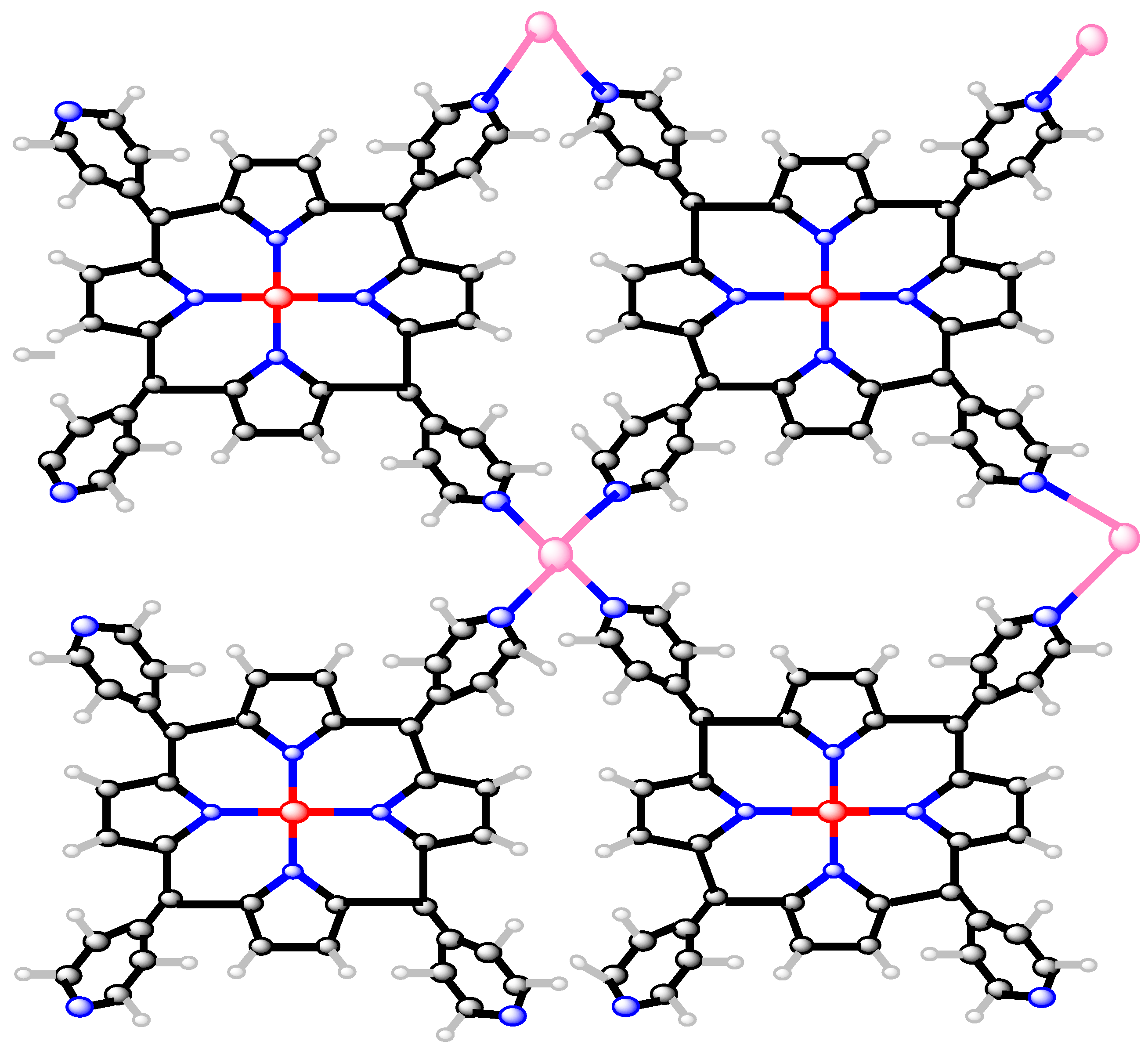
4. Metal–Organic Framework
- The first -Banhatti entropy ofLet be a metal–organic framework. Then, using Equation (1) and Table 3, the first K-Banhatti polynomial isNow, we compute the 1st K-Banhatti entropy of () by using Table 3 and Equation (35) in Equation (10) in the following way:After simplification, we obtain
- The second -Banhatti entropy of
- The first -hyper Banhatti entropy ofLet be a metal–organic framework. Then, using Equation (3) and Table 3, the first K-hyper Banhatti polynomial isNow, we compute the first K-hyper Banhatti entropy of by using Table 3 and Equation (40) in Equation (12) in the following way:After simplification, we obtain
- The second -hyper Banhatti entropy ofLet be a metal–organic framework. Then, by using Equation (4) and Table 3, the second K-Banhatti polynomial isNow, we compute the second K-hyper Banhatti entropy of by using Table 3 and Equation (42) in Equation (13) in the following way:After simplification, we obtain
- The first redefined Zagreb entropy ofLet be a metal–organic framework. Then, using Equation (5) and Table 3, the first redefined Zagreb polynomial isTaking the first derivative of Equation (44) at , we obtain the first redefined Zagreb indexNow, we compute the first redefined Zagreb entropy using Table 3 and Equation (45) in Equation (14) in the following way:After simplification, we obtain
- The second redefined Zagreb entropy ofLet be a metal–organic framework. Then, using Equation (6) and Table 3, the second redefined Zagreb polynomial isTaking the first derivative of Equation (46) at , we obtain the second redefined Zagreb indexNow, we compute the second redefined Zagreb entropy by using Table 3 and Equation (47) in Equation (15) in the following way:After simplification, we obtain
- The third redefined Zagreb entropy ofLet be a metal–organic framework. Then, using Equation (7) and Table 3, the third redefined Zagreb polynomial isTaking the first derivative of Equation (48) at , we obtain the third redefined Zagreb indexNow, we compute the third redefined Zagreb entropy by using Table 3 and Equation (49) in Equation (16) in the following way:After simplification, we obtain
- Atom-bond sum connectivity entropy ofLet NbO be a network of a niobium oxide molecule. Then, using Equation (8) and Table 1, the atom-bond sum connectivity polynomial isTaking the first derivative of Equation (50) at , we obtain the atom-bond sum connectivity index
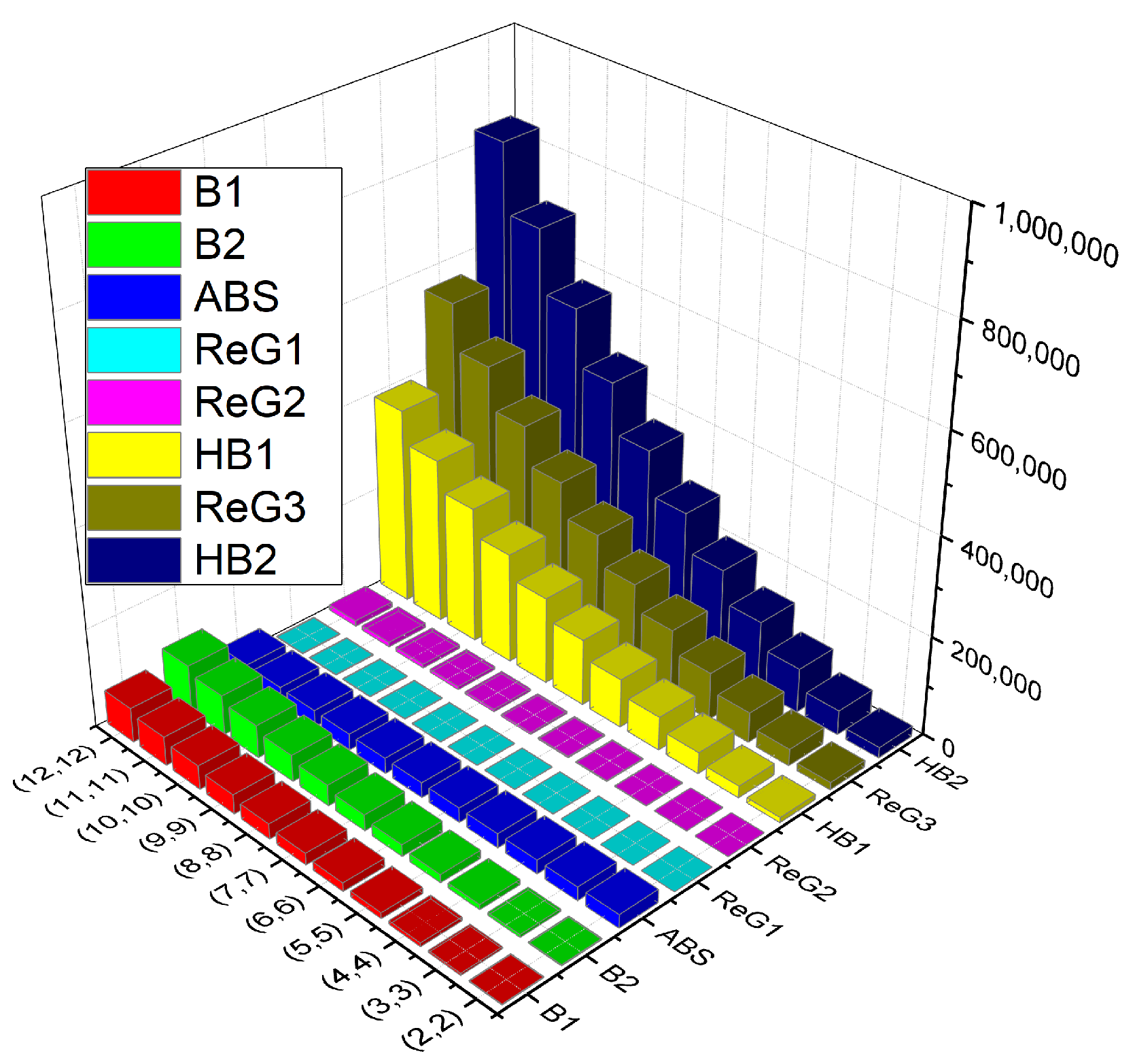
Comparison
5. Conclusions
Author Contributions
Funding
Institutional Review Board Statement
Informed Consent Statement
Data Availability Statement
Conflicts of Interest
References
- Liu, J.B.; Zhang, T.; Wang, Y.; Lin, W. The Kirchhoff index and spanning trees of Möbius/cylinder octagonal chain. Discret. Appl. Math. 2022, 307, 22–31. [Google Scholar] [CrossRef]
- Liu, J.B.; Bao, Y.; Zheng, W.T.; Hayat, S. Network coherence analysis on a family of nested weighted n-polygon networks. Fractals 2021, 29, 2150260. [Google Scholar] [CrossRef]
- Liu, J.B.; Zhao, J.; He, H.; Shao, Z. Valency-based topological descriptors and structural property of the generalized sierpiński networks. J. Stat. Phys. 2019, 177, 1131–1147. [Google Scholar] [CrossRef]
- Liu, J.-B.; Wang, C.; Wang, S.; Wei, B. Zagreb indices and multiplicative zagreb indices of eulerian graphs. Bull. Malays. Math. Sci. Soc. 2019, 42, 67–78. [Google Scholar] [CrossRef]
- Liu, J.B.; Zhao, J.; Min, J.; Cao, J. The Hosoya index of graphs formed by a fractal graph. Fractals 2019, 27, 1950135. [Google Scholar] [CrossRef]
- Liu, J.B.; Pan, X.F. Minimizing Kirchhoff index among graphs with a given vertex bipartiteness. Appl. Math. Comput. 2016, 291, 84–88. [Google Scholar] [CrossRef]
- Liu, J.B.; Pan, X.F.; Yu, L.; Li, D. Complete characterization of bicyclic graphs with minimal Kirchhoff index. Discret. Appl. Math. 2016, 200, 95–107. [Google Scholar] [CrossRef]
- Chu, Y.M.; Khan, A.R.; Ghani, M.U.; Ghaffar, A.; Mustafa Inc. Computation of Zagreb Polynomials and Zagreb Indices for Benzenoid Triangular & Hourglass System. Polycycl. Aromat. Compd. 2022, in press. [Google Scholar] [CrossRef]
- Wiener, H. Structural determination of paraffin boiling points. J. Am. Chem. Soc. 1947, 69, 17–20. [Google Scholar] [CrossRef] [PubMed]
- Vukičević, D.; Gašperov, M. Bond additive modeling 1. Adriatic indices. Croat. Chem. Acta 2010, 83, 243–260. [Google Scholar]
- Kulli, V.R. On K Banhatti indices of graphs. J. Comput. Math. Sci. 2016, 7, 213–218. [Google Scholar]
- Kulli, V.R.; On, K. On K hyper-Banhatti indices and coindices of graphs. Int. Res. J. Pure Algebra 2016, 6, 300–304. [Google Scholar]
- Kulli, V.R. On multiplicative K Banhatti and multiplicative K hyper-Banhatti indices of V-Phenylenic nanotubes and nanotorus. Ann. Pure Appl. Math. 2016, 11, 145–150. [Google Scholar]
- Ranjini, P.S.; Lokesha, V.; Usha, A. Relation between phenylene and hexagonal squeeze using harmonic index. Int. J. Graph Theory 2013, 1, 116–121. [Google Scholar]
- Saeed, N.; Long, K.; Mufti, Z.S.; Sajid, H.; Rehman, A. Degree-based topological indices of boron b12. J. Chem. 2021, 2021, 5563218. [Google Scholar] [CrossRef]
- Ali, A.; Furtula, B.; Redžepović, I.; Gutman, I. Atom-bond sum-connectivity index. J. Math. Chem. 2022, 60, 2081–2093. [Google Scholar] [CrossRef]
- Shannon, C.E. A mathematical theory of communication. Bell Syst. Tech. J. 1948, 27, 379–423. [Google Scholar] [CrossRef] [Green Version]
- Alam, A.; Ghani, M.U.; Kamran, M.; Shazib Hameed, M.; Hussain Khan, R.; Baig, A.Q. Degree-Based Entropy for a Non-Kekulean Benzenoid Graph. J. Math. 2022, 2022, 2288207. [Google Scholar]
- Rashid, T.; Faizi, S.; Zafar, S. Distance based entropy measure of interval-valued intuitionistic fuzzy sets and its application in multicriteria decision making. Adv. Fuzzy Syst. 2018, 2018, 3637897. [Google Scholar] [CrossRef]
- Hayat, S. Computing distance-based topological descriptors of complex chemical networks: New theoretical techniques. Chem. Phys. Lett. 2017, 688, 51–58. [Google Scholar] [CrossRef]
- Hu, M.; Ali, H.; Binyamin, M.A.; Ali, B.; Liu, J.B.; Fan, C. On distance-based topological descriptors of chemical interconnection networks. J. Math. 2021, 2021, 5520619. [Google Scholar] [CrossRef]
- Anjum, M.S.; Safdar, M.U. K Banhatti and K hyper-Banhatti indices of nanotubes. Eng. Appl. Sci. Lett. 2019, 2, 19–37. [Google Scholar] [CrossRef]
- Asghar, A.; Rafaqat, M.; Nazeer, W.; Gao, W. K Banhatti and K hyper Banhatti indices of circulant graphs. Int. J. Adv. Appl. Sci. 2018, 5, 107–109. [Google Scholar] [CrossRef]
- Kulli, V.R.; Chaluvaraju, B.; Boregowda, H.S. Connectivity Banhatti indices for certain families of benzenoid systems. J. Ultra Chem. 2017, 13, 81–87. [Google Scholar] [CrossRef]
- Manzoor, S.; Siddiqui, M.K.; Ahmad, S. On entropy measures of molecular graphs using topological indices. Arab. J. Chem. 2020, 13, 6285–6298. [Google Scholar] [CrossRef]
- Liu, R.; Yang, N.; Ding, X.; Ma, L. An unsupervised feature selection algorithm: Laplacian score combined with distance-based entropy measure. In Proceedings of the 2009 Third International Symposium on Intelligent Information Technology Application, Nanchang, China, 21–22 November 2009; IEEE: Picataway, NJ, USA, 2009; Volume 3. [Google Scholar]
- Nico, C.; Monteiro, T.; Graça, M.P. Niobium oxides and niobates physical properties: Review and prospects. Prog. Mater. Sci. 2016, 80, 1–37. [Google Scholar] [CrossRef]
- Wurster, B.; Grumelli, D.; Hotger, D.; Gutzler, R.; Kern, K. Driving the oxygen evolution reaction by nonlinear cooperativity in bimetallic coordination catalysts. J. Am. Chem. Soc. 2016, 138, 3623–3626. [Google Scholar] [CrossRef] [PubMed]


| Types of Atom Bonds | ||||
|---|---|---|---|---|
| Cardinality of Atom bonds | 16 | 2(2st-s-t) |
| ABS | ||||||||
|---|---|---|---|---|---|---|---|---|
| (2,2) | 552 | 872 | 3528 | 9320 | 58 | 136.34 | 5680 | 75.920117 |
| (3,3) | 1180 | 1944 | 7860 | 22,344 | 113 | 291.77 | 13,152 | 160.400806 |
| (4,4) | 2040 | 3432 | 13,880 | 408,872 | 186 | 504.34 | 23,664 | 275.748201 |
| (5,5) | 3132 | 5336 | 21,588 | 64,904 | 277 | 774.058 | 37,216 | 421.962304 |
| (6,6) | 4456 | 7656 | 30,984 | 94,440 | 386 | 1100.91 | 53,808 | 599.043115 |
| (7,7) | 6012 | 10,392 | 42,068 | 129,480 | 513 | 1484.9 | 73,440 | 806.990632 |
| (8,8) | 7800 | 13,544 | 54,840 | 170,024 | 658 | 1926.1 | 96,112 | 1045.804857 |
| (9,9) | 9820 | 17,112 | 69,300 | 216,072 | 821 | 2424.3 | 121,824 | 1315.48579 |
| (10,10) | 12,072 | 21,096 | 85,448 | 267,624 | 1002 | 2979.7 | 150,576 | 1616.03343 |
| (11,11) | 14,556 | 25,496 | 103,284 | 324,680 | 1201 | 3592.3 | 182,368 | 1947.447777 |
| (12,12) | 17,272 | 30,312 | 122,808 | 387,240 | 1418 | 4262.1 | 217,200 | 2309.728831 |
| Types of Atom Bonds | ||||
|---|---|---|---|---|
| Cardinality of Atom bonds | 4(2st − s − t + 1) |
| (2,2) | 1868 | 2529 | 10,542 | 21,573 | 296 | 307.03 | 14832 | 27,339.22 |
| (3,3) | 4264 | 5793 | 24,122 | 49,725 | 444 | 700.71 | 34008 | 27,686.67 |
| (4,4) | 7636 | 10,401 | 43,286 | 89,685 | 592 | 1256.40 | 61152 | 28,173.03 |
| (5,5) | 11,984 | 16,353 | 68,034 | 141,453 | 740 | 1974.09 | 96,264 | 28,798.29 |
| (6,6) | 17,308 | 23,649 | 98,366 | 205,029 | 888 | 2853.77 | 139,344 | 29,562.45 |
| (7,7) | 23,608 | 32,289 | 134,282 | 280,413 | 1036 | 3895.46 | 190,392 | 30,465.50 |
| (8,8) | 30,884 | 42,273 | 175,782 | 367,605 | 1184 | 5099.14 | 249,408 | 31,507.46 |
| (9,9) | 39,136 | 53,601 | 222,866 | 466,605 | 1332 | 6464.83 | 316,392 | 32,688.32 |
| (10,10) | 48,364 | 66,273 | 275,534 | 577,413 | 1480 | 7992.51 | 391,344 | 34,008.08 |
| (11,11) | 58,568 | 80,289 | 333,786 | 700,029 | 1628 | 9682.20 | 474,264 | 35,466.73 |
| (12,12) | 69,748 | 95,649 | 397,622 | 834,453 | 1776 | 11,533.89 | 565,152 | 37,064.29 |
Publisher’s Note: MDPI stays neutral with regard to jurisdictional claims in published maps and institutional affiliations. |
© 2022 by the authors. Licensee MDPI, Basel, Switzerland. This article is an open access article distributed under the terms and conditions of the Creative Commons Attribution (CC BY) license (https://creativecommons.org/licenses/by/4.0/).
Share and Cite
Ghani, M.U.; Sultan, F.; Tag El Din, E.S.M.; Khan, A.R.; Liu, J.-B.; Cancan, M. A Paradigmatic Approach to Find the Valency-Based K-Banhatti and Redefined Zagreb Entropy for Niobium Oxide and a Metal–Organic Framework. Molecules 2022, 27, 6975. https://doi.org/10.3390/molecules27206975
Ghani MU, Sultan F, Tag El Din ESM, Khan AR, Liu J-B, Cancan M. A Paradigmatic Approach to Find the Valency-Based K-Banhatti and Redefined Zagreb Entropy for Niobium Oxide and a Metal–Organic Framework. Molecules. 2022; 27(20):6975. https://doi.org/10.3390/molecules27206975
Chicago/Turabian StyleGhani, Muhammad Usman, Faisal Sultan, El Sayed M. Tag El Din, Abdul Rauf Khan, Jia-Bao Liu, and Murat Cancan. 2022. "A Paradigmatic Approach to Find the Valency-Based K-Banhatti and Redefined Zagreb Entropy for Niobium Oxide and a Metal–Organic Framework" Molecules 27, no. 20: 6975. https://doi.org/10.3390/molecules27206975