
Increased Arctic NO3− Availability as a Hydrogeomorphic Consequence of Permafrost Degradation and Landscape Drying

 , , , ,
Abstract
:1. Introduction
2. Materials and Methods
3. Results
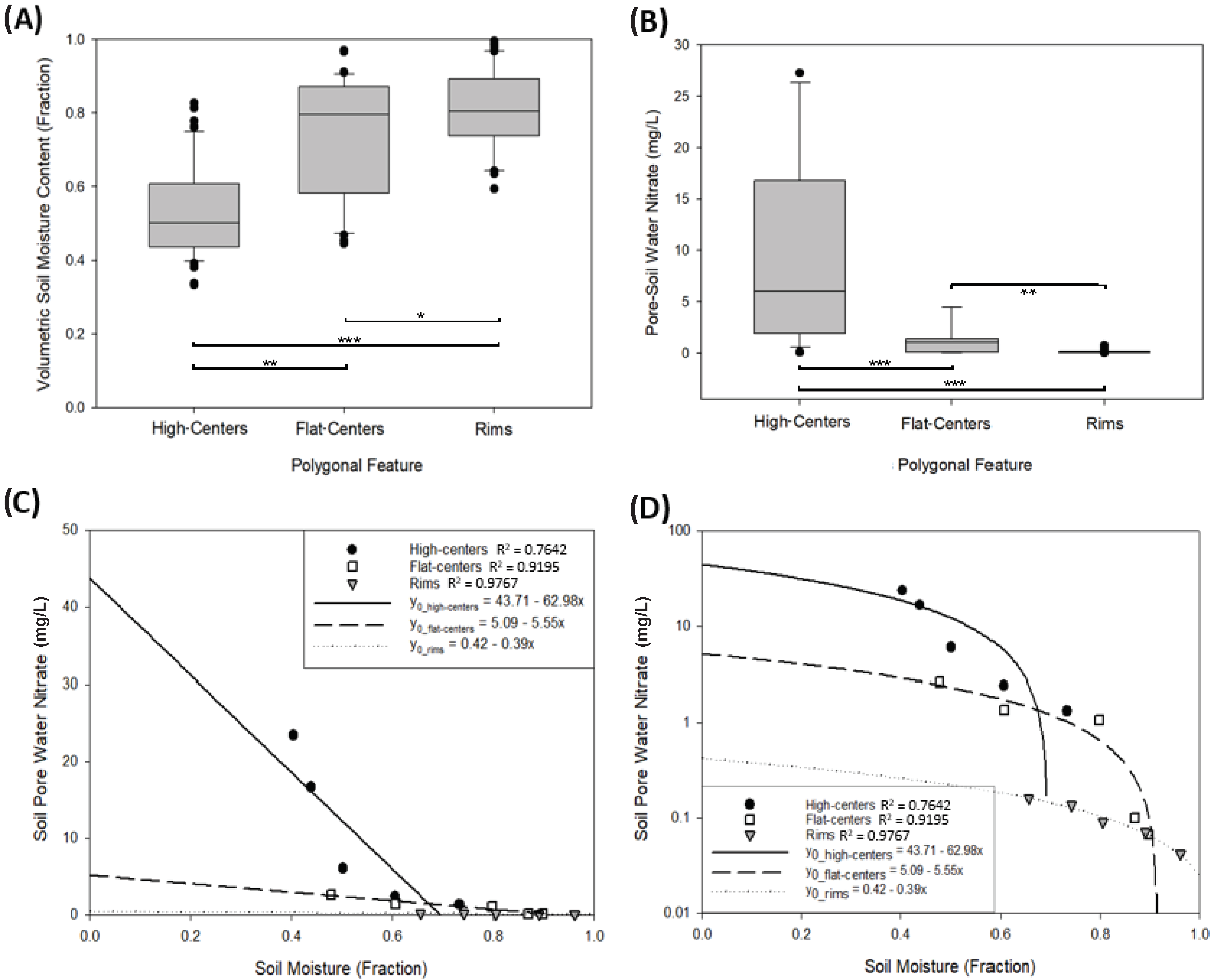
3.1. Soil NO3− and Soil Moisture Distributions across Polygonal Microtopographic Features
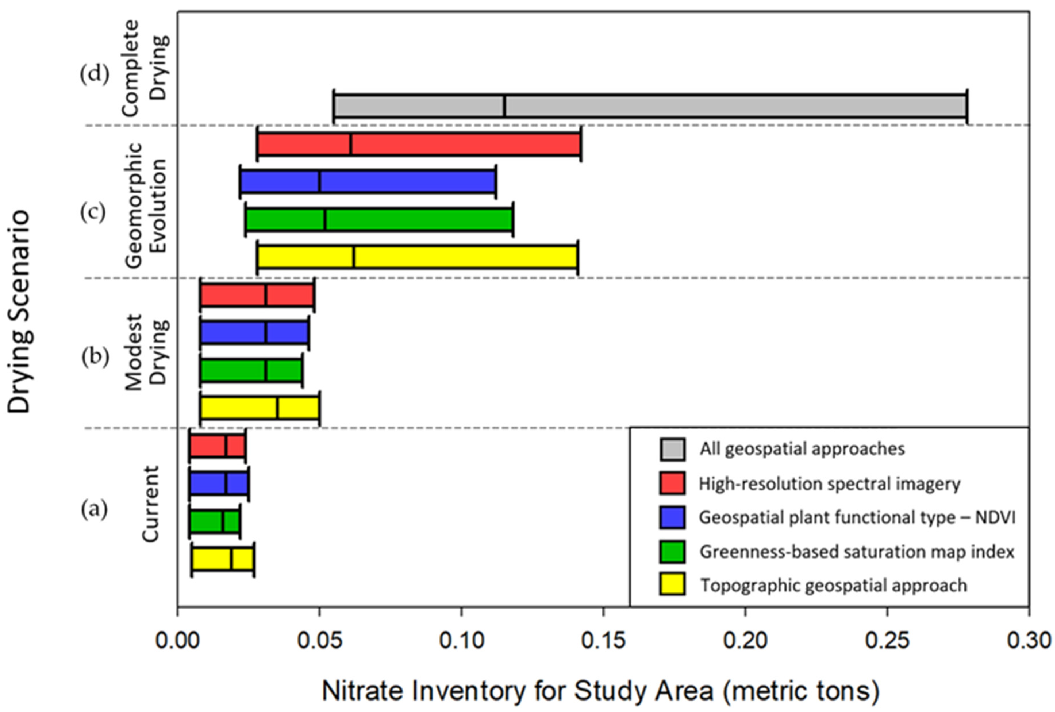
3.2. NO3− Inventories from Study Area
4. Discussion
5. Conclusions
Author Contributions
Funding
Institutional Review Board Statement
Informed Consent Statement
Data Availability Statement
Acknowledgments
Conflicts of Interest
Appendix A
Appendix A.1. Sources of Nitrate
Appendix A.2. Detailed Methods
Defining the Relationship between Soil Moisture and NO3−
- The 0–10% distribution of NO3− with the 90–100% distribution of soil moisture;
- The 10–25% distribution of NO3− with the 75–90% distribution of soil moisture;
- The 25–50% distribution of NO3− with the 50–75% distribution of soil moisture;
- The 50–75% distribution of NO3− with the 25–50% distribution of soil moisture;
- The 75–90% distribution of NO3− with the 10–25% distribution of soil moisture;
- The 90–100% distribution of NO3− with the 0–10% distribution of soil moisture.

| Feature | Parameter | n | Min | 10% | 25% | 50% | 75% | 90% | Max |
|---|---|---|---|---|---|---|---|---|---|
| Rims | NO3− (mg/L) | 31 | 0.022 | 0.042 | 0.070 | 0.090 | 0.135 | 0.160 | 0.730 |
| Volumetric soil moisture fraction | 152 | 0.594 | 0.656 | 0.742 | 0.805 | 0.890 | 0.961 | 0.995 | |
| Flat-Centers | NO3− (mg/L) | 49 | 0.051 | 0.066 | 0.099 | 1.052 | 1.347 | 2.000 | 4.442 |
| Volumetric soil moisture fraction | 97 | 0.445 | 0.478 | 0.606 | 0.797 | 0.870 | 0.897 | 0.970 | |
| High-Centers | NO3− (mg/L) | 65 | 0.082 | 1.320 | 2.398 | 6.000 | 16.609 | 23.400 | 27.260 |
| Volumetric soil moisture fraction | 87 | 0.333 | 0.403 | 0.438 | 0.502 | 0.605 | 0.733 | 0.827 | |
| All Features | NO3− (mg/L) | 145 | 0.022 | 0.051 | 0.080 | 0.120 | 0.615 | 4.460 | 27.260 |
| Volumetric soil moisture fraction | 336 | 0.333 | 0.4431 | 0.513 | 0.732 | 0.850 | 0.903 | 0.995 |
Appendix A.3. Geospatial Methods
Appendix A.3.1. Topographic, Polygon Geomorphology-Based Saturation Map
- Troughs: microtopographic low regions along with the polygon boundaries;
- Rims: high regions in flat- and low-centered polygons;
- Low-centers: low regions within flat- and low-centered polygons; and
- High-centers: high regions within high-centered polygons.
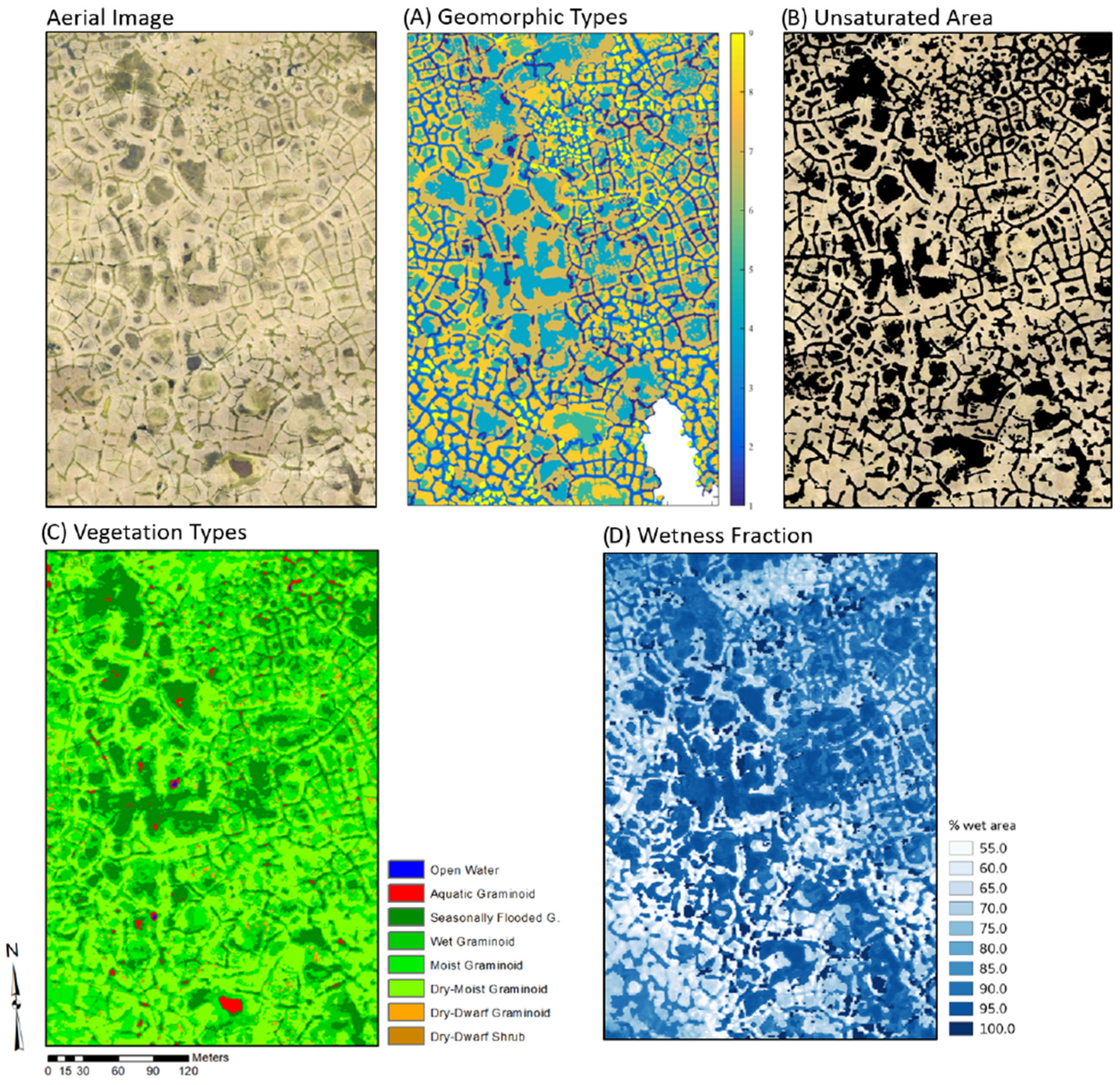
Appendix A.3.2. Greenness-Based Saturation Map Index
- (x,y) is likely to be pond if gI(x,y) < threshold_gI_l, or max(R,G,B) < threshold_mx_l, or sat(x,y) < threshold_sat;
- (x,y) is likely to be vegetation if gI(x,y) > threshold_gI_h, or max(R,G,B) < threshold_mx_h;
- If none of these criteria are met, (x,y) is likely to be dry.
Appendix A.3.3. Plant Functional Type (NDVI)
Appendix A.3.4. High-Resolution Spectral Imagery:
Appendix A.4. NO3− Inventories
| Geospatial Method | Topographic Geospatial Approach [38] | Greenness and Saturation Based Map [41,42,43] | Plant Community Types—NDVI [44,45] | High-Resolution Spectral Imagery [16,46] | Average |
|---|---|---|---|---|---|
| Technique Description | Microtopography was extracted from LiDAR DEM, by removing the average elevation relative to the centers of polygons to classify troughs, rims, low-centers, flat-centers, and high-centers. | Color orthomosaic was used to infer greenness and saturation indexes that serve to identify saturated vs. unsaturated land cover. | Total coverage by different plant communities that are associated with varying soil moisture regimes: wet graminoids, dry graminoids, forbs, lichens, and mosses. Classification based on sub-meter multi-spectral imagery and NDVI. | Multi-spectral data from WorldView-2 satellites and airborne LiDAR-derived elevation data coupled with wet/dry graminoid distributions. | - |
| % Area Unsaturated | 61.3 | 59.7 | 62.4 | 57.6 | 60.3 |
| Current NO3− Inventory (metric tons) | 0.016 | 0.014 | 0.015 | 0.015 | 0.015 |
| Modest Drying NO3− Inventory (metric tons) | 0.038 | 0.035 | 0.036 | 0.036 | 0.036 |
| Geomorphic Evolution NO3− Inventory (metric tons) | 0.062 | 0.050 | 0.048 | 0.060 | 0.055 |
| Complete Drying NO3− Inventory (metric tons) | 0.122 | 0.122 | 0.122 | 0.122 | 0.122 |
References
- Jorgenson, M.T.; Harden, J.; Kanevskiy, M.; O’Donnell, J.; Wickland, K.; Weing, S.; Manies, K.; Zhuang, Q.; Shur, Y.; Striegl, R.; et al. Reorganization of vegetation, hydrology and soil carbon after permafrost degradation across heterogeneous boreal landscapes Environ. Res. Lett. 2013, 8. [Google Scholar] [CrossRef]
- O’Donnell, J.; Douglas, T.; Barker, A.; Guo, L. Changing biogeochemical cycles of organic carbon, nitrogen, phosphorus, and trace elements in Arctic rivers. In Arctic Hydrology, Permafrost and Ecosystems; Yang, D., Kane, D.L., Eds.; Springer: Cham, Denmark, 2021; pp. 315–348. [Google Scholar] [CrossRef]
- McClelland, J.W.; Stieglitz, M.; Pan, F.; Holmes, R.M.; Peterson, B.J. Recent changes in nitrate and dissolved organic carbon export from the upper Kuparuk River, North Slope, Alaska. J. Geophys. Res. 2007, 111, G04S60. [Google Scholar] [CrossRef]
- Salmon, V.G.; Soucy, P.; Mauritz, M.; Celis, G.; Natali, S.M.; Mack, M.C.; Schuur, E.A.G. Nitrogen availability increases in a tundra ecosystem during five years of experimental permafrost thaw. Glob. Chang. Biol. 2016, 22, 1927–1941. [Google Scholar] [CrossRef] [PubMed]
- Liu, X.-Y.; Koba, K.; Koyama, L.A.; Hobbie, S.E.; Weiss, M.S.; Inagaki, Y.; Shaver, G.R.; Giblin, A.E.; Hobara, S.; Nadelhoffer, K.J.; et al. Nitrate is an important nitrogen source for Arctic tundra plants. PNAS USA 2018, 115, 3398–3403. [Google Scholar] [CrossRef] [Green Version]
- Norby, R.J.; Sloan, V.L.; Iversen, C.M.; Childs, J. Controls on fine-scale spatial and temporal variability of plant available inorganic nitrogen in a polygonal tundra landscape. Ecosystems 2018, 22, 528–543. [Google Scholar] [CrossRef] [Green Version]
- Biasi, C.; Wanek, W.; Rusalimova, O.; Kaiser, C.; Meyer, H.; Barsukov, P.; Richter, A. Microtopography and plant-cover controls on nitrogen dynamics in hummock tundra. Arct. Antarct. Alp. Res. 2005, 37, 435–443. [Google Scholar] [CrossRef] [Green Version]
- Keuper, F.; van Bodegom, P.M.; Dorrepaal, E.; Weedon, J.T.; van Hal, J.; van Logtestijn, R.S.P.; Aerts, R. A frozen feast: Thawing permafrost increases plant-available nitrogen in subarctic peatlands. Glob. Chang. Biol. 2012, 18, 1998–2007. [Google Scholar] [CrossRef]
- Barnes, R.T.; Williams, M.W.; Parman, J.N.; Hill, K.; Caine, N. Thawing glacial and permafrost features contribute to nitrogen export from Green Lakes Valley, Colorado Front Range, USA. Biogeochemistry 2014, 117, 413–430. [Google Scholar] [CrossRef] [Green Version]
- Salmon, V.G.; Breen, A.L.; Kumar, J.; Lara, M.J.; Thornton, P.E.; Wullschleger, S.D.; Iversen, C.M. Alder distribution and expansion across a tundra hillslope: Implications for local N cycling. Front. Plant Sci. 2019, 10. [Google Scholar] [CrossRef]
- McCaully, R.E.; Arendt, C.A.; Newman, B.D.; Salmon, V.G.; Heikoop, J.M.; Wilson, C.J.; Sevanto, S.; Wales, N.A.; Perkins, G.B.; Marina, O.C.; et al. High temporal and spatial nitrate variability on an Alaskan hillslope dominated by alder shrubs. Cryosphere 2022, 16, 1889–1901. [Google Scholar] [CrossRef]
- Hiltbrunner, E.; Aerts, R.; Buhlmann, T.; Huss-Danell, K.; Magnusson, B.; Myrold, D.D.; Reed, C.; Sigurdsson, B.D.; Korner, C. Ecological consequences of the expansion of N2-fixing plants in cold biomes. Oecologia 2014, 176, 11–24. [Google Scholar] [CrossRef] [PubMed] [Green Version]
- Mekonnen, Z.A.; Riley, W.J.; Grant, R.F. Accelerated nutrient cycling and increased light competition will lead to 21st century shrub expansion in North American Arctic Tundra. J. Geophys. Res. Biogeosci. 2017, 123, 1683–1701. [Google Scholar] [CrossRef]
- Gamon, J.A.; Huemmrich, K.F.; Stone, R.S.; Tweedie, C.E. Spatial and temporal variation in primary productivity (NDVI) of coastal Alaskan tundra: Decreased vegetation growth following earlier snowmelt. Remote Sens. Environ. 2013, 129, 144–153. [Google Scholar] [CrossRef] [Green Version]
- Lara, M.J.; Nitze, I.; Grosse, G.; Martin, P.; McGuire, A.D. Reduced arctic tundra productivity linked with landform and climate change interactions. Sci. Rep. 2018, 8. [Google Scholar] [CrossRef] [PubMed]
- Lara, M.J.; McGuire, A.D.; Euskirchen, E.S.; Tweedie, C.E.; Hinkle, K.M.; Skurikhin, V.E.; Romanovsky, V.E.; Grosse, G.; Bolton, W.R.; Genet, H. Polygonal tundra geomorphological change in response to warming alters future CO2 and CH4 flux on the Barrow Peninsula. Glob. Chang. Biol. 2015, 21, 1634–1651. [Google Scholar] [CrossRef]
- Chapin, F.S.; Fetcher, N.; Kielland, K.; Everett, K.R.; Linkins, A.E. Productivity and nutrient cycling of Alaskan tundra: Enhancement by flowing soil water. Ecology 1988, 69, 693–702. [Google Scholar] [CrossRef]
- Binkley, D.; Stottlemyer, R.; Suarez, F.; Cortina, J. Soil nitrogen availability in some arctic ecosystems in northwest Alaska: Responses to temperature and moisture. Ecoscience 1994, 1, 64–70. [Google Scholar] [CrossRef]
- Stutter, M.I.; Billett, M.F. Biogeochemical controls on stream water and soil solution chemistry in a High Arctic environment. Geoderma 2003, 113, 127–146. [Google Scholar] [CrossRef]
- Frey, K.E.; McClelland, J.W.; Holmes, R.M.; Smith, L.C. Impacts of climate warming and permafrost thaw on the riverine transport of nitrogen and phosphorus to the Kara Sea. J. Geophys. Res. 2007, 112, G04S58. [Google Scholar] [CrossRef]
- Lafrenière, M.; Lamoureux, S.F. Seasonal dynamics of dissolved nitrogen exports from two High Arctic watersheds, Melville Island, Canada. Hydrol. Res. 2008, 39, 324–335. [Google Scholar] [CrossRef]
- Harms, T.K.; Jones, J.B. Thaw depth determines reaction and transport of inorganic nitrogen in valley bottom permafrost soils: Nitrogen cycling in permafrost soils. Glob. Chang. Biol. 2012, 18, 2958–2968. [Google Scholar] [CrossRef] [PubMed]
- Heikoop, J.M.; Throckmorton, H.M.; Newman, B.D.; Perkins, G.B.; Iversen, C.M.; Chowdhury, T.R.; Romanovsky, V.; Graham, D.E.; Norby, R.J.; Wilson, C.J.; et al. Isotopic identification of soil and permafrost nitrate sources in an Arctic tundra ecosystem. J. Geophys. Res. Biogeosci. 2015, 120, 1000–1017. [Google Scholar] [CrossRef]
- Newman, B.D.; Throckmorton, H.; Graham, D.E.; Hubbard, S.S.; Liang, L.; Wu, Y.; Heikoop, J.M.; Herndon, E.M.; Phelps, T.J.; Wilson, C.J.; et al. Microtopographic and depth controls on active layer chemistry in Arctic polygonal ground. Geophys. Res. Lett. 2015, 42, 1808–1817. [Google Scholar] [CrossRef]
- Liljedahl, A.K.; Boike, J.; Daanen, R.N.; Fedorov, A.N.; Frost, G.V.; Grosse, G.; Hinzman, L.D.; Iijma, Y.; Jorgenson, J.C.; Matveyeva, N.; et al. Pan-Arctic ice-wedge degradation in warming permafrost and its influence on tundra hydrology. Nat. Geosci. 2016, 9, 312–318. [Google Scholar] [CrossRef]
- Koch, J.C.; Jorgenson, M.T.; Wickland, K.P.; Kanevskiy, M.; Striegl, R. Ice wedge degradation and stabilization impact ater budgets and nutrient cycling in Arctic trough ponds. J. Geophys. Res: Biogeosci. 2018, 123, 2604–2616. [Google Scholar] [CrossRef]
- Hinzman, L.D.; Deal, C.J.; McGuire, A.D.; Mernild, S.H.; Polyakov, I.V.; Walsh, J.E. Trajectory of the Arctic as an integrated system. Ecol. Appl. 2013, 23, 1837–1868. [Google Scholar] [CrossRef]
- Walvoord, M.A.; Kurylyk, B.L. Hydrologic impacts of thawing permafrost—A review. Vadose Zone J. 2016, 15. [Google Scholar] [CrossRef]
- Leffingwell, E. Ground Ice Wedges: The dominant form of ground-ice on the north coast of Alaska. J. Geol. 1915, 23, 635–654. [Google Scholar] [CrossRef]
- Jorgenson, M.T.; Shur, Y.L.; Pullman, E.R. Abrupt increase in permafrost degradation in Arctic Alaska. Geophys. Res. Lett. 2006, 33, L02503. [Google Scholar] [CrossRef]
- Dafflon, B.; Hubbard, S.; Ulrich, C.; Peterson, J.; Wu, Y.; Wainwright, H.; Kneafsey, T.J. Geophysical estimation of shallow permafrost distribution and properties in an ice-wedge polygon-dominated Arctic tundra region. Geophysics 2016, 81, WA247–WA263. [Google Scholar] [CrossRef]
- Engstrom, R.; Hope, A.; Kwon, H.; Stow, D.; Zamolodchikov, D. Spatial distribution of near surface soil moisture and its relationship to microtopography in the Alaskan Arctic coastal plain. Hydrol. Res. 2005, 36, 219–234. [Google Scholar] [CrossRef]
- Woo, M.K.; Guan, X.J. Hydrological connectivity and seasonal storage change of tundra ponds in a polar oasis environment: Canadian High Arctic. Permafr. Periglac. Process. 2006, 17, 209–323. [Google Scholar] [CrossRef]
- Gersper, P.L.; Alexander, V.; Barkley, S.A.; Barsdate, R.J.; Flint, P.S. The soils and their nutrients. In An Arctic Ecosystem: The Coastal Tundra at Barrow, Alaska; Brown, J., Ed.; Dowden, Hutchinson and Ross: Stroudsburg, PA, USA, 1980; pp. 219–254. [Google Scholar]
- Seeberg-Elverfeldt, J.; Schlüter, M.; Feseker, T.; Kölling, M. Rhizon sampling of porewaters near the sediment-water interface of aquatic systems. Limnol. Oceanogr. Meth. 2005, 3, 361–371. [Google Scholar] [CrossRef]
- Romano, N. Soil moisture at local scale: Measurements and simulations. J. Hydrol. 2014, 514, 6–20. [Google Scholar] [CrossRef]
- Barsdate, R.J.; Alexander, V. The nitrogen balance of Arctic Tundra: Pathways, rates, and environmental implications. J. Environ. Qual. 1975, 4, 111–117. [Google Scholar] [CrossRef]
- Wainwright, H.M.; Dafflon, B.; Smith, L.J.; Hahn, M.S.; Curtis, J.B.; Wu, Y.; Ulrich, C.; Peterson, J.E.; Torn, M.S.; Hubbard, S.S. Identifying multiscale zonation and assessing the relative importance of polygon geomorphology on carbon fluxes in an Arctic tundra ecosystem. J. Geophys. Res. Biogeosci. 2015, 120, 788–808. [Google Scholar] [CrossRef]
- Wu, Y.; Ulrich, C.; Kneafsey, T.J.; Lopez, R.; Chou, C.; Geller, J.; McKnight, K.; Dafflon, B.; Soom, F.; Peterson, J.; et al. Depth-resolved physiochemical characteristics of active layer and permafrost soils in an Arctic polygonal tundra region. J. Geophys. Res. Biogeosci. 2018, 123, 1136–1386. [Google Scholar] [CrossRef] [Green Version]
- Hubbard, S.S.; Gangodagamage, C.; Dafflon, B.; Wainwright, H.; Peterson, J.; Gusmeroli, A.; Urlich, C.; Wu, Y.; Wilson, C.J.; Rowland, J.C.; et al. Quantifying and relating land-surface and subsurface variability in permafrost environments using LiDAR and surface geophysical datasets. Hydrogeol. J. 2013, 21, 149–169. [Google Scholar] [CrossRef]
- Dafflon, B.; Oktem, R.; Peterson, J.; Ulrich, C.; Tran, A.P.; Romanovsky, V.; Hubbard, S.S. Coincident aboveground and belowground autonomous monitoring to quantify covariability in permafrost, soil, and vegetation properties in Arctic tundra. J. Geophys. Res. Biogeosci. 2017, 122, 1321–1342. [Google Scholar] [CrossRef] [Green Version]
- Hobbie, J.; Shaver, G.; Rastetter, E.; Cherry, J.; Goetz, S.; Guay, K.; Gould, W.; Kling, G. Ecosystem responses to climate change at a Low Arctic and a High Arctic long-term research site. Ambio 2017, 46, 160–173. [Google Scholar] [CrossRef] [Green Version]
- Wainwright, H.M.; Oktem, R.; Dafflon, B.; Dengel, S.; Curtis, J.B.; Torn, M.S.; Cherry, J.; Hubbard, S.S. High-resolution spatio-temporal estimation of net ecosystem exchange in ice-wedge polygon tundra using in situ sensors and remote sensing data. Land 2021, 10, 722. [Google Scholar] [CrossRef]
- Villarreal, S.; Hollister, R.D.; Johnson, D.R.; Lara, M.J.; Webber, P.J.; Tweedie, C.E. Tundra vegetation change near Barrow, Alaska (1972–2010). Environ. Res. Lett. 2012, 7. [Google Scholar] [CrossRef]
- Andresen, C.G.; Lara, M.J.; Tweedie, C.E.; Lougheed, V.L. Rising plant-mediated methane emissions from arctic wetlands. Glob. Chang. Biol. 2017, 23, 1128–1139. [Google Scholar] [CrossRef] [PubMed]
- Langford, Z.; Kumar, J.; Hoffman, F.M.; Norby, R.J.; Wullschleger, S.D.; Sloan, V.L.; Iversen, C.M. Mapping Arctic Plant Functional Type distributions in the Barrow Environmental Observatory using WorldView-2 and LiDAR Datasets. Remote Sens. 2016, 8, 733. [Google Scholar] [CrossRef] [Green Version]
- Andresen, C.G.; Lawrence, D.M.; Wilson, C.J.; McGuire, A.D.; Koven, C.; Schaefer, K.; Jafarov, E.; Peng, S.; Chen, X.; Gouttevin, I.; et al. Soil moisture and hydrology projections of the permafrost region – A model intercomparison. Cryosphere 2020, 14, 445–459. [Google Scholar] [CrossRef] [Green Version]
- Keller, K.; Blum, J.D.; Kling, G.W. Geochemistry of soils and streams on surfaces of varying ages in Arctic Alaska. Arct. Antarct. Alp. Res. 2007, 39, 84–98. [Google Scholar] [CrossRef]
- Keller, K.; Blum, J.D.; Kling, G.W. Stream geochemistry as an indicator of increasing permafrost thaw depth in an arctic watershed. Chem. Geol. 2010, 273, 76–81. [Google Scholar] [CrossRef]
- Lipson, D.A.; Schmidt, S.K.; Monson, R.K. Links between microbial population dynamics and nitrogen availability in an alpine ecosystem. Ecology 1999, 85, 1623–1631. [Google Scholar] [CrossRef]
- Lecher, A.L.; Chien, C.-T.; Paytan, A. Submarine groundwater discharge as a source of nutrients to the North Pacific and Arctic coastal ocean. Mar. Chem. 2016, 186, 167–177. [Google Scholar] [CrossRef] [Green Version]
- Kendrick, M.R.; Huryn, A.D.; Bowden, W.B.; Deegan, L.A.; Findlay, R.H.; Hershey, A.E.; Peterson, B.J.; Benes, J.P.; Schuett, E.B. Linking permafrost thaw to shifting biogeochemistry and food web resources in an arctic river. Glob. Chang. Biol. 2018, 24, 5738–5750. [Google Scholar] [CrossRef]
- Billings, W.D.; Peterson, K.M.; Luken, J.O.; Mortensen, D.A. Interaction of increasing atmospheric carbon dioxide and soil nitrogen on the carbon balance of tundra microcosms. Oecologia 1984, 65, 26–29. [Google Scholar] [CrossRef] [PubMed]
- Schuur, E.A.G.; McGuire, A.D.; Schädel, C.; Grosse, G.; Harden, J.W.; Hayes, D.J.; Hugelius, G.; Koven, C.D.; Kuhry, P.; Lawrence, D.M.; et al. Climate change and the permafrost carbon feedback. Nature 2015, 520, 171–179. [Google Scholar] [CrossRef]
- Ramm, E.; Liu, C.; Wang, X.; Yue, H.; Zhang, W.; Pan, Y.; Schloter, M.; Gschwendtner, S.; Mueller, C.W.; Hu, B.; et al. The forgotten nutrient—The role of nitrogen in permafrost soils of Northern China. Adv. Atmos. Sci. 2020, 37, 793–799. [Google Scholar] [CrossRef]
- Ramm, E.; Liu, C.; Ambus, P.; Butterbach-Bahl1, K.; Hu, B.; Martikainen, P.J.; Marushchak, M.E.; Mueller, C.W.; Rennenberg, H.; Schloter, M.; et al. A review of the importance of mineral nitrogen cycling in the plant-soil-microbe system of permafrost-affected soils—changing the paradigm. Environ. Res. Lett. 2022, 17. [Google Scholar] [CrossRef]
- Yang, Z.-P.; Gao, J.-X.; Zhao, L.; Xu, X.-L.; Ouyang, H. Linking thaw depth with soil moisture and plant community composition: Effects of permafrost degradation on alpine ecosystems on the Qinghai-Tibet Plateau. Plant Soil 2013, 367, 687–700. [Google Scholar] [CrossRef]
- Finger, R.A.; Turetsky, M.R.; Kielland, K.; Ruess, R.W.; Mack, M.C.; Euskirchen, E.S. Effects of permafrost thaw on nitrogen availability and plant-soil interactions in boreal Alaskan lowland. J. Ecol. 2016, 104, 1542–1554. [Google Scholar] [CrossRef]
- Faucher, B.; Lacelle, D.; Davila, A.; Pollard, W.; Fisher, D.; McKay, C.P. Physicochemical and Biological Controls on Carbon and Nitrogen in Permafrost from an Ultraxerous Environment, McMurdo Dry Valleys of Antarctica. J. Geophys. Res. 2017, 122, 1293–2604. [Google Scholar] [CrossRef]


Publisher’s Note: MDPI stays neutral with regard to jurisdictional claims in published maps and institutional affiliations. |
© 2022 by the authors. Licensee MDPI, Basel, Switzerland. This article is an open access article distributed under the terms and conditions of the Creative Commons Attribution (CC BY) license (https://creativecommons.org/licenses/by/4.0/).
Share and Cite
Arendt, C.A.; Heikoop, J.M.; Newman, B.D.; Wilson, C.J.; Wainwright, H.; Kumar, J.; Andersen, C.G.; Wales, N.A.; Dafflon, B.; Cherry, J.; et al. Increased Arctic NO3− Availability as a Hydrogeomorphic Consequence of Permafrost Degradation and Landscape Drying. Nitrogen 2022, 3, 314-332. https://doi.org/10.3390/nitrogen3020021
Arendt CA, Heikoop JM, Newman BD, Wilson CJ, Wainwright H, Kumar J, Andersen CG, Wales NA, Dafflon B, Cherry J, et al. Increased Arctic NO3− Availability as a Hydrogeomorphic Consequence of Permafrost Degradation and Landscape Drying. Nitrogen. 2022; 3(2):314-332. https://doi.org/10.3390/nitrogen3020021
Chicago/Turabian StyleArendt, Carli A., Jeffrey M. Heikoop, Brent D. Newman, Cathy J. Wilson, Haruko Wainwright, Jitendra Kumar, Christian G. Andersen, Nathan A. Wales, Baptiste Dafflon, Jessica Cherry, and et al. 2022. "Increased Arctic NO3− Availability as a Hydrogeomorphic Consequence of Permafrost Degradation and Landscape Drying" Nitrogen 3, no. 2: 314-332. https://doi.org/10.3390/nitrogen3020021