Signal-to-Noise Ratio Improvement for Multiple-Pinhole Imaging Using Supervised Encoder–Decoder Convolutional Neural Network Architecture

Abstract

Digital image devices have been widely applied in many fields, such as individual recognition and remote sensing. The captured image is a degraded image from the latent observation, where the degradation processing is affected by some factors, such as lighting and noise corruption. Specifically, noise is generated in the processing of transmission and compression from the unknown latent observation. Thus, it is essential to use image denoising techniques to remove noise and recover the latent observation from the given degraded image. In this research, a supervised encoder–decoder convolution neural network was used to fix image distortion stemming from the limited accuracy of inverse filter methods (Wiener filter, Lucy–Richardson deconvolution, etc.). Particularly, we will correct image degradation that mainly stems from duplications arising from multiple-pinhole array imaging.

1. Introduction

A pinhole camera is a lens-less camera with a small aperture (pinhole) that utilizes the “camera obscura” effect. There are several advantages to using a pinhole camera over a conventional lens camera: a wider angular field, no linear distortion, and an infinite depth of focus. On the other side of the coin, there are also disadvantages, such as dim images and a consequently long exposure time in order to gather enough energy on the detector. Another disadvantage is low spatial resolution, which stems from the finite width of the pinhole. The pinhole diameter determines some of the optical characteristics of the pinhole camera, such as signal-to-noise ratio (SNR) and the resolution of the image. There is a tradeoff between these two characteristics, which manifests in a high SNR in a large pinhole diameter as opposed to a high resolution in a small pinhole diameter.

Many methods have been proposed over the years to improve spatial resolution and light intensity whilst preserving the advantages of pinhole optics. Some of the methods proposed are the use of camera films, highly sensitive detectors, and coded aperture imaging (CAI) [1]. The CAI method uses a multi-pinhole [2] matrix in order to encode the latent observation by obtaining an image from multiple pinholes, and it requires a decoding process involving digital or optical decoding to extract the latent observation. In CAI, each pinhole has a small diameter; however, the sum of signals from all the pinholes compensates the low light intensity from the small diameter of each pinhole. Other techniques utilizing the CAI method are cyclic array, mosaic pattern, random array, off-axis Fresnel zone plate, and uniformly redundant array [3,4]. However, the multiple-pinhole mask leads to an overlap of images in the detector plane. This overlapping is partially corrected using Wiener filtering and smart design of the pinhole array, but traces of the duplications remain [5,6,7].

Artificial neural networks (ANNs) are computational network models, inspired by biological brain data processing [8,9,10]. Deep learning (DL) is a class of machine-learning techniques that uses multilayered artificial neural networks for automated analysis of signals or data [9,11]. The name comes from the general structure of deep neural networks, which consist of several layers of artificial neurons stacked one after the other. These models have dramatically improved the performance of many machine-learning tasks, such as speech and image recognition. In recent years, more and more studies have begun to integrate deep learning with optical systems [12,13].

In our work, we present a combination of a multi-pinhole matrix with a DL method to overcome the pinhole camera’s problems, obtain high SNR whilst maintaining high resolution, and remove the noise stems from the limited abilities of inverse filtering. With the proposed DL method, we improved the quality and resolution of the received image.

2. Materials and Methods

In our previous research, we presented a new approach of a multivariable coded aperture (VCA) design for far-field and near-field imaging applications [14,15,16]. The imaging system was based on the time-multiplexing method using a variable multi-pinhole array. The unique variable array design enabled us to overcome the spatial frequencies cutoff and the small terms in the Fourier transform that exist in a standard multi-pinhole array. The overall pinhole positions were designed to avoid spatial frequencies loss.

However, traces of duplications remained using Wiener filtering in the reconstruction process. Moreover, because the pinholes mask most of the photons coming from the object to the camera, the dynamic range was limited. This limitation led to low contrast and improper color gamut.

In the presented work, a combination of a VCA with a deep-convolutional neural network was used to remove the noise stems from the limited abilities of pinhole imaging and inverse filtering. The proposed method led to a higher signal-to-noise ratio, contrast, and resolution.

2.1. Experimental Setup

In our setup, a projector screened an image on a diffuser. The light from the diffuser scattered through the pinhole array and hit the camera’s detector. We used a projector and a diffuser to create the object (it is also possible to use a screen or an illumination of a physical object). On the diffuser, each time, we projected an image from the MNIST dataset and captured a frame on the camera detector after the pinhole array.

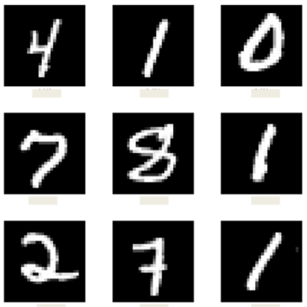
In this experiment, the MNIST (Modified National Institute of Standards and Technology) handwritten digit database was used. This is a database for handwritten digit classification. Each greyscale image was 28 × 28 pixels, representing the digits 0–9. This dataset consisted of 60,000 training images and 10,000 test images. One can see in Figure 1 an example from the MNIST database.

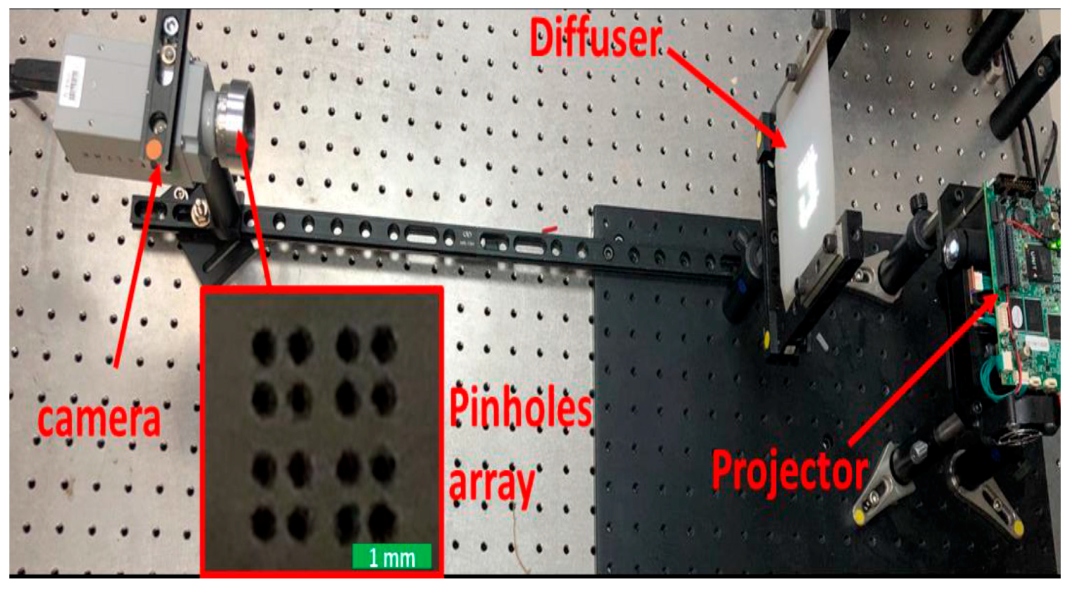
The configuration setup is depicted in Figure 2. This setup consists of a projector and a diffuser; it is also possible to use a screen or an illumination of a physical object.

The projector position is followed by the diffuser. The distance between the diffuser and the projector was determined by the maximum size and resolution of the object. The diffuser was placed as close as possible to create an object with maximum resolution. The projector lens was focused onto the diffuser to obtain sharp images.

A square uniform object (200 × 200 pixels) was projected in order to determine the size of each pixel in the projection system. In this setup, a square with a size of 2.1 μm was used, which means that each pixel size on the diffuser was equal to about 100 μm.

The pinhole array was mounted in front of the camera at a distance of 2.58 cm from the camera sensor. The pinhole array was mounted with the camera at a distance of 43.5 cm from the diffuser (object). The distance between the pinhole array and the diffuser determined magnification by the ratio of $-\frac{v}{u}$, where $v$ is the distance between the pinhole array and the camera detector, and $u$ is the distance between the object and the pinhole array.

2.2. Calibration

To find the pinhole positions on the detector, a single point with the size of 10 pixels (about 1 mm on the diffuser) was projected. In the camera, an image of 16 points was obtained (as the number of pinholes).

The camera was positioned where the center of the pinhole array was in the center of the detector. The frame with these 16 points was captured with the camera.

The center of each point was found, and the PSF matrix of the system was created (the PSF matrix size is the size of the image, in which all the elements are zero except the locations of the point centers, where the value is 1).

When using the proposed system, one must pay attention to the following: lack of synchronization between the camera and the projection system will result in blurring or appearance of different images in the same frame. To avoid this, make sure that the projection time between images is up to twice the exposure time of the camera detector. Additionally, make sure there is no staging of camera detectors, as this may result in loss of spatial information and impair image quality. In order to obtain the best improvement, the physical size and the geometric resolution of the camera detector must meet the optical requirements of the system. The pinhole array creates image duplicates of the object in space, and therefore, the detector size should be large enough to capture the main duplications. In addition, the geometric resolution, the size of the detector pixel, should not be lower than the optical resolution of the single pinhole.

2.3. Creating the Dataset

The PSF of the system was used to create the Wiener filter. The filter was calculated by:

$$H=\frac{G^{*}}{G·G^{*}+N}$$

(1)

where G is the CTF and N is the spectrum of the noise. The noise is considered the standard deviation of the image when a black screen is projected.

On the diffuser, each time, an image was projected from the MNIST dataset, and a frame was captured with the camera.

Next, Wiener filtering was performed on the Fourier transform of each image. Then, a reverse Fourier transform was performed on the result. The processed images were saved in the same order as the original images.

2.4. Dataset Preparation for the Neural Network

The original images were resized to the size of the processed images. The processed images, the resized images, and the original images were split into 2 groups: train 70% and test 30%. The images from the train and the test groups were split into batch sizes of 128 images per batch. The learning process was performed using TensorFlow, the machine learning platform, on GPU RTX 2080 Ti.

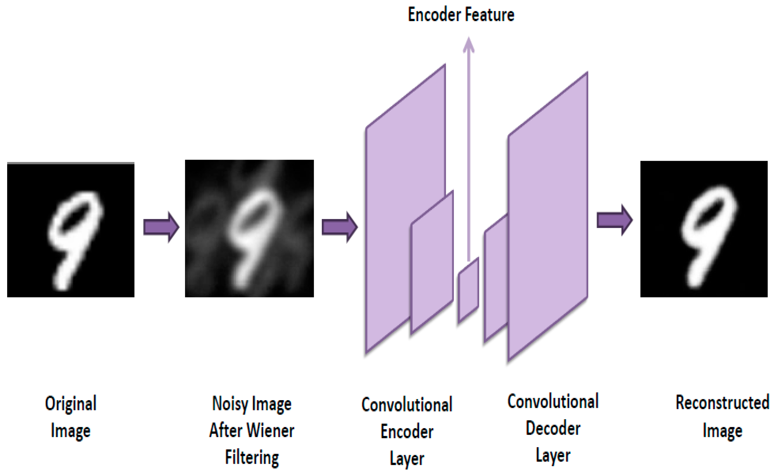
2.5. Convolutional Neural Network Architecture

The convolution neural network was built using the following architecture: an input layer with a shape of (100, 100, 1); a convolution layer with an output shape of (100, 100, 32); a batch normalization layer; a max-pooling layer with an output shape of (50, 50, 32); a convolution layer with an output shape of (50, 50, 64); a batch normalization layer; a max-pooling layer with an output shape of (25, 25, 64); a convolution layer with an output shape of (25, 25, 64); a batch normalization layer; an up-sampling layer with an output shape of (50, 50, 64); a convolution layer with an output shape of (50, 50, 32); a batch normalization layer; an up-sampling layer with an output shape of (100, 100, 32); and a convolution layer with an output shape of (100, 100, 1). One can see this structure in Figure 3.

In the train batch, the processed images were taken and were used as input for the network. An equivalent number of the original images were used at the end of the network as the ground truth.

Rectified linear unit (ReLU) was used as the activation function in the convolution layers:

$$f\left(x\right)=x^{+}=\max \left(0,x\right)$$

(2)

where x is the input to a neuron. The nearest neighbor algorithm was used in the up-sampling layers. The network was trained for 4 epochs, with Adam optimization algorithm and with binary cross-entropy loss (BCE), which compare the changes between the processed image and the original image:

$$L_{bce}=-\frac{1}{M}{\displaystyle \sum }_{m=1}^M[y_m\times \log \left(h_{\theta }\left(x_m\right)\right)+(1-y_m)\times \log \left(1-h_{\theta }\left(x_m\right)\right)]$$

(3)

where M is the number of training examples, $y_m$ is the target for training example number m, $x_m$ is the input for training example m, and $h_{\theta }$ is the model with neural network weights θ.

3. Results and Discussion

In this experiment, the MNIST dataset was used in the multiple-pinhole imaging system. All 70,000 images of the dataset were projected onto the diffuser and captured by the lens-less CCD camera after moving through the pinhole array, as can be seen in Figure 2.

One can see in Figure 1 the original image. The image produced after passing through the pinhole imaging system is presented in Figure 4A. Figure 4B presents the same image after using the inverse Wiener filter. The figures show that traces of the duplications still exist, despite the use of this filter.

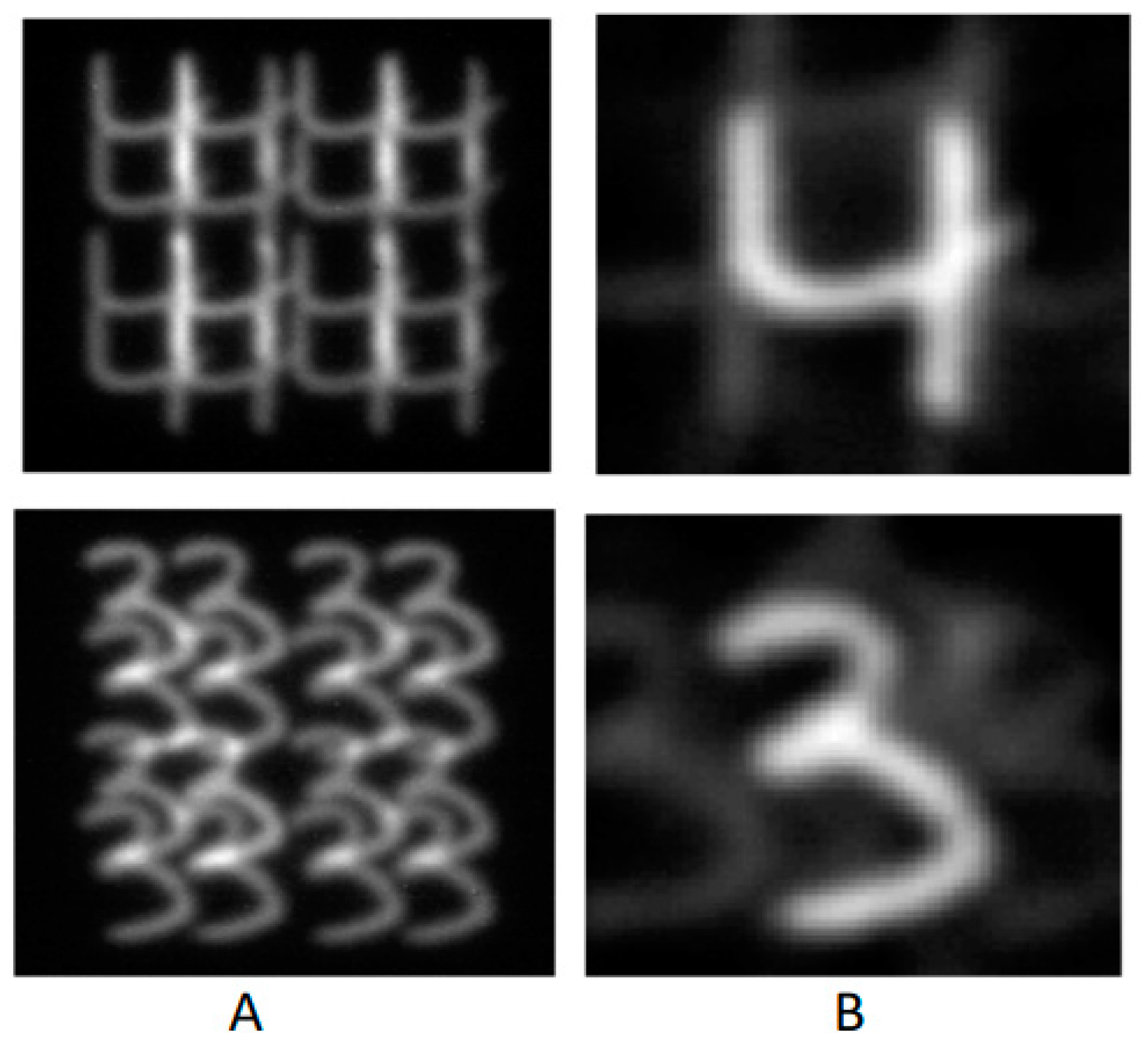
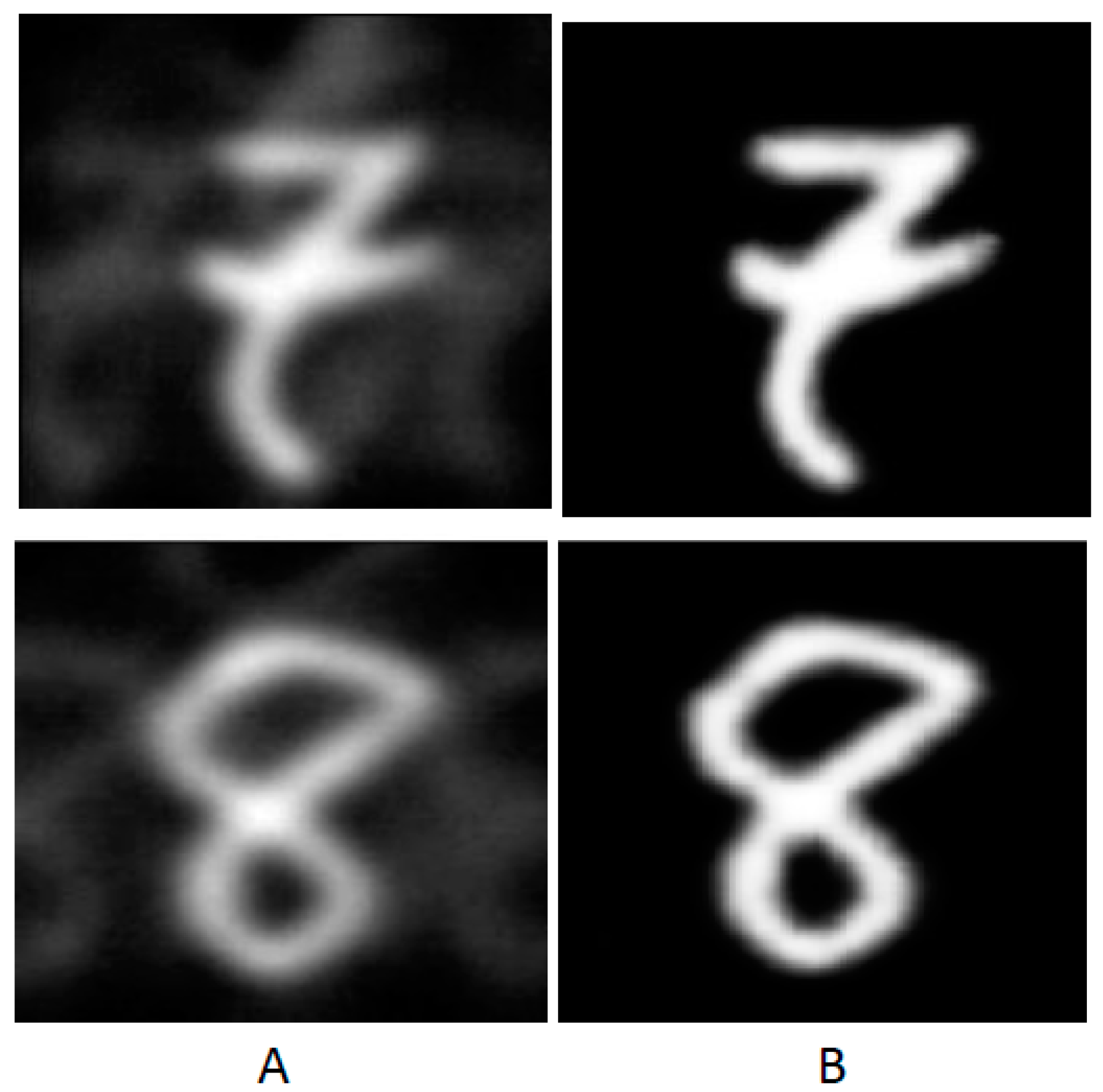
After using the proposed DL method, the duplication traces that exist in Figure 5A were removed, as presented in Figure 5B.

The SNR improvement that the DL method performed on the image can be seen in Figure 5 by comparing this image to the original image. In detail, the output image of the convolution neural network, Figure 5B, is more similar to the original image, compared to the image presented in Figure 5A. The reason for this improvement is that the convolution neural network was trained with binary cross-entropy loss (BCE) to minimize the changes between the processed image and the original image. By minimizing these changes, the SNR was improved. In this scenario, the signal is the original image as a ‘ground truth’ to the CNN, and the noise is the difference between each pixel in the original images and in the processed images. By this process, the image distortion that occurred to the original image due to the pinhole module was corrected using the convolution neural network. This difference between the images can be calculated using mean squared error (MSE):

$$MSE\left(x, y\right)=\frac{1}{n}{\displaystyle \sum }_{i=0}^{n-1}{\left(x_i-y_i\right)}^2$$

(4)

where y is the original image, x is the processed image, n is the number of pixels, and $x_i$ and $y_i$ represent the intensity in the i-th pixel. The MSE between Figure 5A and the original images is 0.01 for digit 7 and 0.0086 for digit 8, while the MSE between Figure 5B and the original images is 0.0005 for digit 7 and 0.0004 for digit 8. The reduction in the MSE stems from the CNN.

One can see that there are artifacts in the Figure 5A images, in comparison to the original image that is presented in Figure 3. Most of these artifacts were dismissed after using the DL method. This convolution neural network enhanced the clarity of the image by recognizing the artifacts that the pinhole array made as a noise, relative to the original image. The main goal of this method was to restore the original image that was corrupted by the pinhole system and semi-reconstructed by inverse Wiener filtering. Furthermore, the network enhanced the image clarity by removing all the duplicates that were made by the pinhole and were not removed by the Wiener filter.

In our future work, we will examine an expansion of the proposed DL method by using various pinhole pattern sets, using complex images as input for the system, and developing end-to-end deep learning solutions that can handle the entire reconstruction process without Wiener filtering.

In this paper, we presented a pinhole imaging system combined with deep learning algorithms which can, at the same time, improve image clarity and SNR for a shorter exposure time.

In the optical spectrum, the pinhole system still cannot compete with an imaging system with a lens, but at shorter wavelengths, such as in the gamma and X-ray spectrums, where no lenses are present, the potential is great. In the future, we will also conduct experiments in the field of gamma and X-rays to reduce the radiation dose absorbed in patients while improving artificial intelligence algorithms in order to meet these requirements.