Combined Jones–Stokes Polarimetry and Its Decomposition into Associated Anisotropic Characteristics of Spatial Light Modulator


1
Applied Optics & Spectroscopy Laboratory, Department of Physics, Kumaun University, SSJ Campus, Almora 263601, Uttarakhand, India
2
Department of Physics, Soban Singh Jeena (SSJ) University, Almora 263601, Uttarakhand, India
*
Author to whom correspondence should be addressed.
Photonics 2022, 9(3), 195; https://doi.org/10.3390/photonics9030195
Submission received: 31 January 2022
/
Revised: 11 March 2022
/
Accepted: 15 March 2022
/
Published: 17 March 2022
(This article belongs to the Special Issue Polarized Light and Optical Systems)
Abstract
:Jones–Stokes polarimetry is a robust in vitro polarimetric technique that can be used to investigate the anisotropic properties of a birefringent medium. The study of spatially resolved Jones matrix components of an object is a heuristic approach to extract its phase and polarization information. However, direct interpretation of Jones matrix elements and their decomposition into associated anisotropic properties of a sample is still a challenging research problem that needs to be investigated. In this paper, we experimentally demonstrate combined Jones–Stokes polarimetry to investigate the amplitude, phase, and polarization modulation characteristics of a twisted nematic liquid crystal spatial light modulator (TNLC-SLM). The anisotropic response of the SLM is calibrated for its entire grayscale range. We determine the inevitable anisotropic properties viz., diattenuation, retardance, isotropic absorption, birefringence, and dichroism, which are retrieved from the measured Jones matrices of the SLM using Jones polar decomposition and a novel algebraic approach for Jones matrix decomposition. The results of this study provide a complete polarimetric calibration of the SLM within the framework of its anisotropic characteristics.
1. Introduction
Polarimetry is emerging as a conventional imaging technique in optics, especially in non-invasive imaging applications [1]. Polarimetric imaging techniques (PIT) have paved the way in determining the anisotropic characteristics of birefringent crystals [2,3], biological samples [4,5], LCDs [6,7], etc. In general, a sample can be treated as either homogeneous or non-homogeneous depending on its structural configuration. Based on this categorization, polarimetry encompasses two main techniques, i.e., Jones matrix imaging and Mueller matrix imaging. Jones matrix imaging is used to retrieve the phase information of an object, whereas Mueller matrix imaging is employed to study samples containing significant depolarization [8]. Among the aforementioned crucial applications, PITs play a promising role in LCD characterization. LCDs are considered as homogeneous birefringent samples; hence, Jones matrix imaging is preferred over other polarimetric techniques for LCD characterization due to their remarkable phase retardation properties [9,10]. The liquid crystal (LC) is a state of matter that exhibits birefringence; that is, it has different refractive indices along different reference axes. When an LCD is placed in an external electric field, it behaves like an electric dipole and tends to align along the direction of the electric field, depending on the strength of the electric field. It provides a tool for controlling the orientation of crystals and, therefore, can control the angle at which incident light propagates through them. It allows for the optimization of relative phase shifts for field components corresponding to crystal rotation.
Spatial light modulators (SLMs) are specifically designed programmable LCDs, which are subjected to the amplitude, phase, and polarization modulation of light [7,11,12]. These optimized modulation characteristics enable the utilization of SLMs as the dynamic optical component in various applications, namely, digital holography [13], metrology [14], and adaptive optics [15]. The working of SLMs is based on the LC principle; that is, the modulation characteristics of the SLM depend on the dipole moment of twisted nematic liquid crystals concerning the applied potential difference between two glass substrates. Hence, TNLC-SLMs can be treated as variable retarders with a fixed fast axis. However, the subtle manufacturing and compact design of SLMs require calibration for their precise applications [12]. Moreover, the ideal polarization response of the SLM for its grayscales can be varied due to various exogenous factors, such as display curvature [16], phase flicker [17,18], and temperature fluctuations [17]. Several techniques have been reported to characterize the amplitude and phase response of the SLM as a function of its grayscales [6,7,8,9,12,14,18,19,20,21,22]. Some interferometric techniques are suggested for the measurement of the Jones matrix of LC displays, but these techniques require a highly coherent source and are very sensitive to external effects, e.g., thermal vibrations and mechanical disturbances [8]. Furthermore, a few studies point out that the state of polarization (SOP) of an input light beam can vary after interacting with an SLM [14,22]. This modulated SOP can alter the polarization response of the SLM [6,14,23]. It is observed that the earlier reported techniques on Jones matrix determination of the SLM require four-shot imaging, i.e., four different sets of measurements [8,24]. In addition, these studies are limited only to basic properties (amplitude and phase) and do not provide comprehensive information about the crucial anisotropic properties, i.e., birefringence, dichroism, and isotropic phase shift of the SLM. One of the recent studies on SLM calibration suggests that only phase calibration is not sufficient to enable the complete polarization response of the SLM [25]. In practice, SLMs are subjected to anisotropic tendencies with respect to their different grayscales. The Jones matrix can be treated as the fingerprint for the phase modulation properties of birefringent samples and, hence, can be further investigated to obtain a robust characterization of the SLM. In this framework, a more heuristic interpretation of Jones matrix elements is required to investigate the anisotropic characteristics of the SLM.
Direct interpretation of Jones matrix elements and their decomposition into basic polarization properties of light can be an efficient approach for characterizing the birefringent properties of the LC-SLM. To the best of the authors’ knowledge, no study has been carried out on the direct anisotropic measurements from the Jones matrix of the SLM to date. In this paper, we characterize the amplitude, phase, and polarization modulation characteristics of a twisted nematic liquid crystal spatial light modulator (TNLC-SLM) for its grayscales using combined Jones–Stokes polarimetry. The anisotropic response of the SLM is calibrated for its entire grayscale range. The Jones matrices of the SLM are experimentally measured using an improvised polarization-sensitive interferometer followed by the Fourier fringe analysis (FFA) technique [26]. Moreover, the essential anisotropic properties, i.e., isotropic absorption (IA), isotropic phase shift (IPS), (linear, circular) birefringence (LB, CB), and (linear, circular) dichroism (LD, CD), were directly retrieved from the measured Jones matrices of the SLM using Jones matrix polar decomposition and a novel algebraic approach to Jones decomposition.
2. Theoretical Background
2.1. Origin of Anisotropic Characteristics of LC-SLM
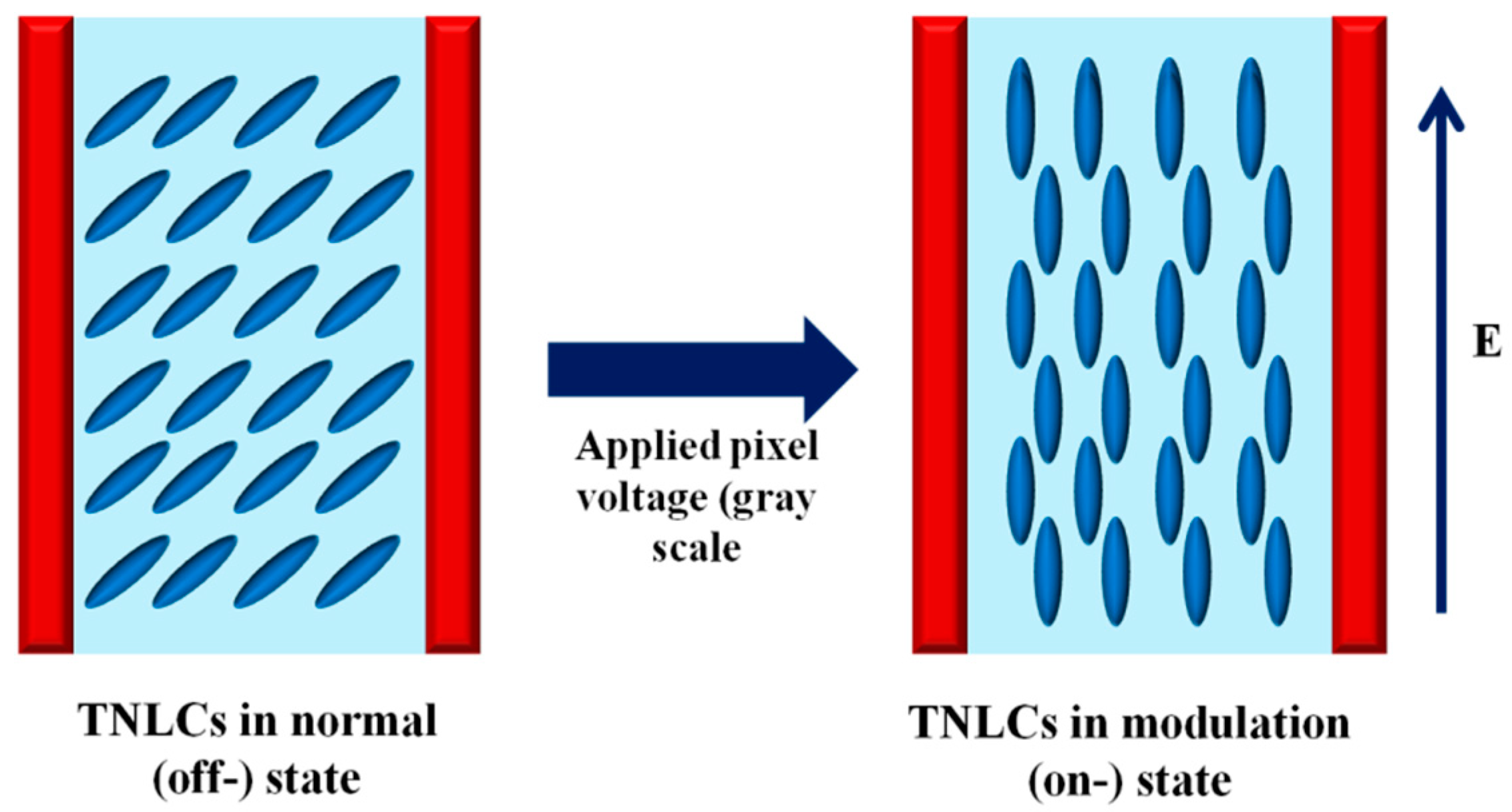
The LC-SLM can exhibit an anisotropic nature due to the relative phase delay for the orthogonal polarization components of its LC array. Let us consider that the SLM is designed to modulate the phase of light along the vertically polarized (y-polarized) light. The phase delay experienced by the SLM is given as
no and ne are the refractive indices for the slow and fast axes of the LC-SLM, respectively, and d is the thickness of the LC cell. The relative rotation of LC molecules of the SLM for applied pixel voltage (grayscale) is shown in Figure 1.
When pixel voltage (grayscale) is applied to the SLM, it provides an additional phase to the y-polarized light, whereas the x-component of light remains unaffected.
The resultant phase of the x-polarized component of light is
The resultant phase of the y-polarized component of light is
Here, is the additional phase due to the applied grayscale of the SLM.
The retardance of the SLM can be defined as
It is clear from Equation (3) that the retardance varies as the applied grayscale is changed for the SLM, and it results in the anisotropic characteristics of the SLM. Therefore, precise calibration of the anisotropic response of the SLM, with respect to its grayscales, is required to obtain complete polarization modulation characterization of the SLM.
2.2. Determination of Jones Matrices of the SLM
When the sample (SLM) is illuminated with a +45° linearly polarized light beam, the output orthogonal field components (Epx and Epy) are given as [9]
Similarly, for the −45° linearly polarized incident light beam, the output orthogonal field components (Emx and Emy) can be given as
The Stokes polarization parameters (SPPs) for the +45° polarized incident light beam are determined from the retrieved electric field components as
Similarly, SPPs for the −45° polarized incident light beam are determined from the retrieved electric field components as
The degree of polarization (DOP) of the output light is determined from the SPPs as
The Jones matrix elements are derived in terms of orthogonal field components as
Equation (8) represents the Jones matrix () of the SLM. The anisotropic properties of the SLM are encoded in and can be retrieved by decomposition of the Jones matrices of the SLM.
2.3. Jones Matrix Decomposition into Anisotropic Properties of the SLM
2.3.1. Polar Decomposition of Jones Matrices
The basic anisotropic characteristics (diattenuation and retardance) can be determined using polar decomposition of Jones matrices as
Here, is the diattenuation matrix and is the retardance matrix of the object.
Let be the eigen values of JD and be the eigen values of JR. Then, the diattenuation (D) and retardance (R) of J are defined by
Other anisotropic properties (IA, IPS, LB, and LD) are retrieved from J by using the linear algebraic method.
2.3.2. Jones Matrix Decomposition Using the Linear Algebraic Method
The Jones matrix of an object can be written as a linear combination of four linearly independent (LI) matrices of order 2 × 2 (α, β, γ and δ) as [27]
The LI matrices (α, β, γ and δ) form the basis of a generalized Jones matrix. The matrix α does not affect the orientation of the incident electric field, whereas the basic operation of the other three matrices, α, β, γ and δ, is to flip the incident electric field with respect to the x-axis and the 45° axis, and to rotate clockwise by an angle of 90°, respectively.
The anisotropic parameters (A, B, C, and D) are defined in terms of the Jones matrices of the sample as
These parameters (A, B, C, and D) represent anisotropic properties of a sample and are summarized in Table 1.
3. Experimental Details
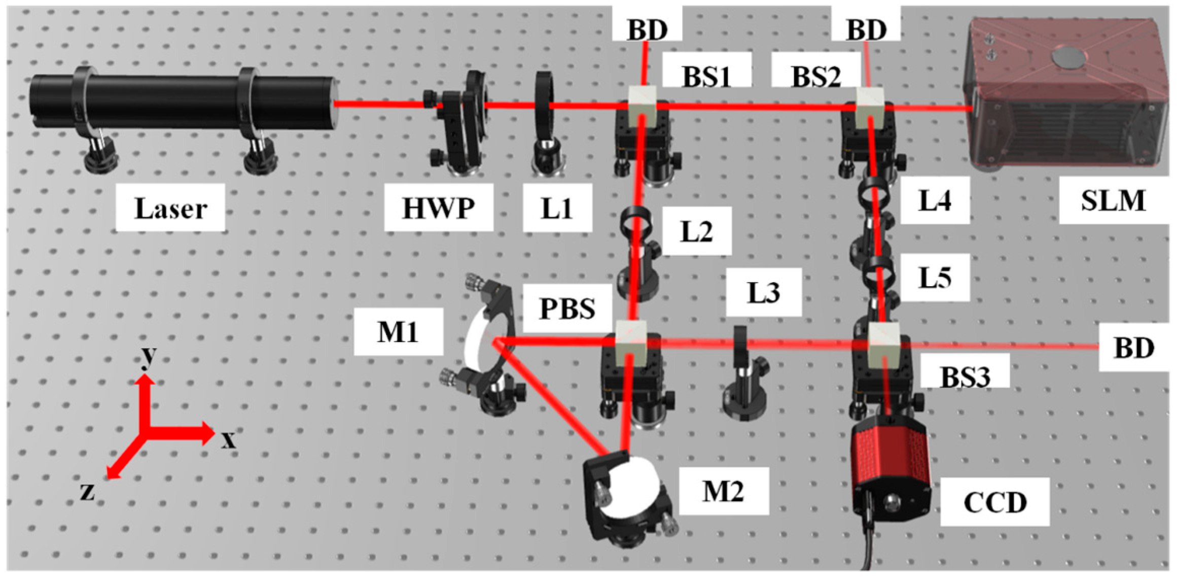
Figure 2 represents the schematic of the experimental measurement of Jones matrices of a reflective-type TNLC-SLM (Holoeye, LC-R720). A plane-polarized light beam with a wavelength of 633 nm coming out of a He-Ne laser is converted into 45° polarized light using a half-wave plate (HWP) and is collimated by a bi-convex lens L1 with a focal length of 200 mm. This collimated beam is then allowed to pass through a polarization interferometer, which consists of three-beam splitters (BSn (n = 1 to 3)), four lenses (Ln (n = 2 to 5)), and a polarizing beam splitter (PBS). The BS1 splits the collimated beam with two equal intensities into two arms of the interferometer, i.e., the reference arm and the object arm. The beam on the reference arm is then introduced into a triangular Sagnac interferometer with the help of lens L2 (focal length 250 mm) and L3 (focal length 250 mm), which consists of a PBS and two mirrors, M1 and M2. The PBS splits light into two counter-propagating orthogonal polarization components. The orthogonal field components emerging from the reference arm (Rx(x,y) and Ry(x,y)) interfere with the corresponding field components emerging from the object arm (Ox(x,y) and Oy(x,y)). This results in a chessboard-like pattern (an interference pattern). This pattern is recorded with a CCD camera (PCO pixel fly, 14 bit, 1392 × 1040 pixels, and a pixel size of 6.45 μm) placed at the image plane.
The recorded interference pattern for input ±45° polarized light can be mathematically represented as
J is the Jones matrix of the SLM and is the output field corresponding to +45° and −45° polarized input light beams, respectively.
We recorded the interference patterns for +45° polarized input light at different grayscales (0, 5, 10, 15 up to 255) of the SLM in the first shot. A similar procedure is followed in the second shot, i.e., for −45° polarized input light. A total of 104 interference patterns were recorded in order to determine the Jones matrices of the SLM with regard to its grayscales.
4. Results and Discussion
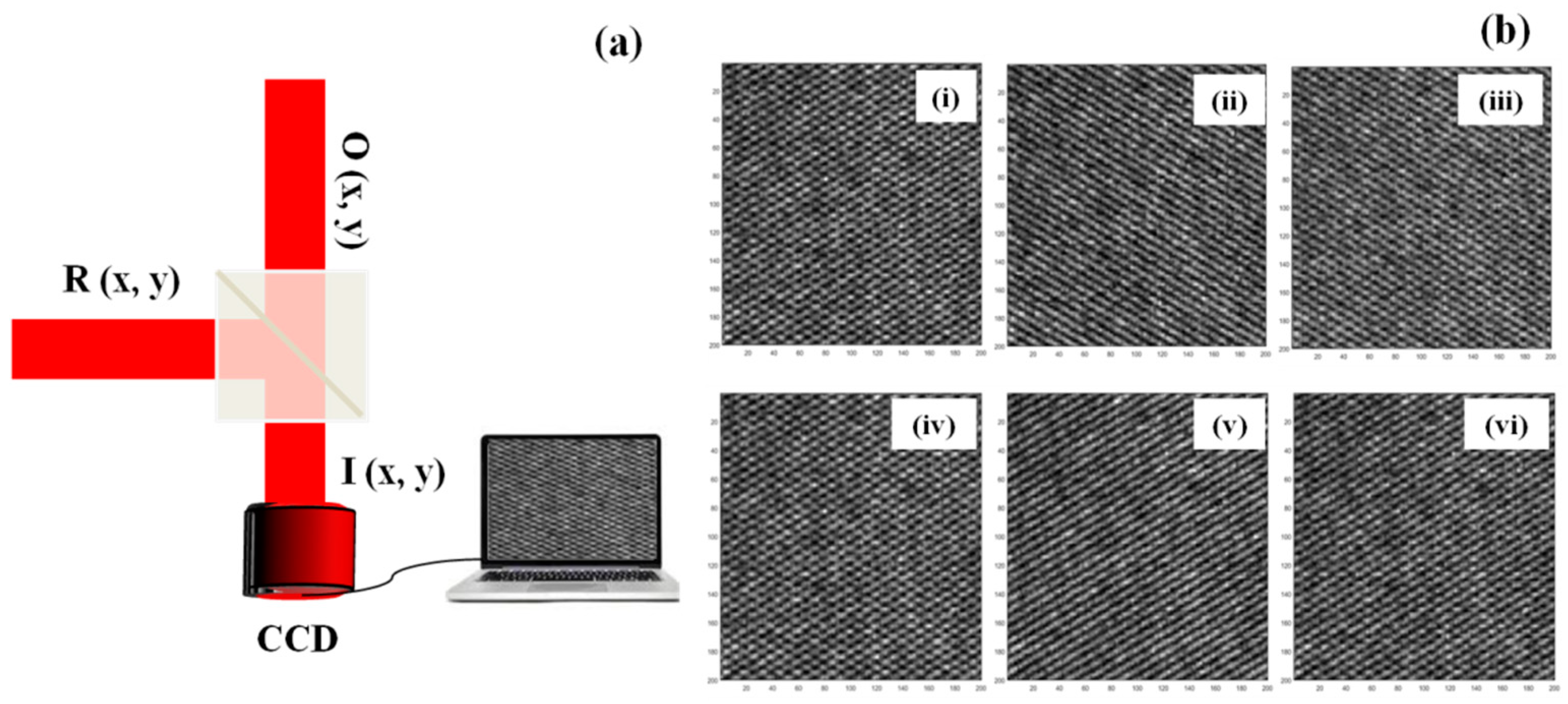
Figure 3a presents the schematic of the recorded hologram (I(x,y)), which is formed from the interference of corresponding polarization components of the reference beam (R(x,y)) and object beam (O(x,y)). Figure 3b presents the recorded interferograms for +45° polarized incident light Figure 3b(i–iii) and −45° polarized light Figure 3b(iv–vi) at three grayscales of the SLM, i.e., 5, 180, and 255, respectively. On examining the fringes at three grayscales, it can be observed that the chessboard-like pattern turns into linear fringes at grayscale 180 Figure 3b(ii,v), and it reappears again as the chessboard-like pattern Figure 3b(iii,vi). This indicates that one of the components of the orthogonal field component of light is converted into a single component at grayscale 180. This implies that the SLM rotates the SOP of input light at different grayscales.
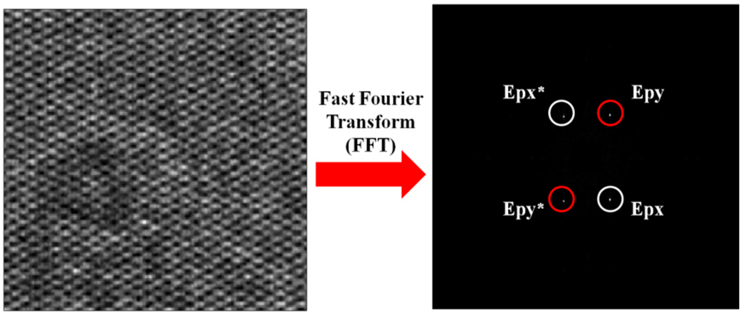
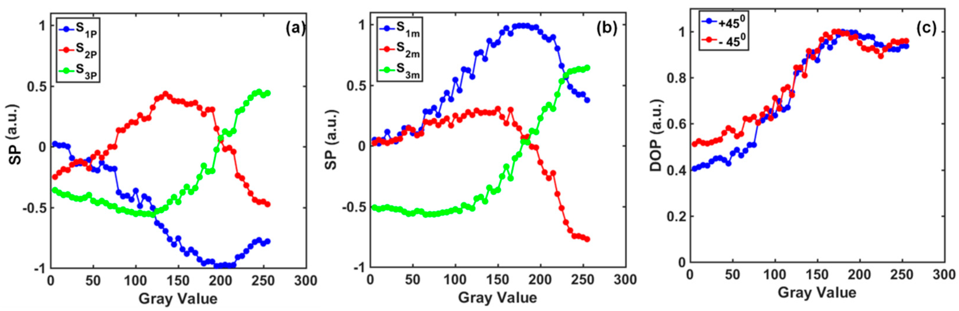
Figure 4 presents the interference pattern and Fourier spectrum corresponding to the recorded interferogram at grayscale 255 for input +45° polarized light. To extract the field components, one of the Fourier peaks was selected and processed using the FFA technique [26]. The output electric field components for the SLM are reported in our previous work [9]. In the next step, the SOP modulation characteristics of the SLM were calibrated using Stokes polarimetry. SPPs of the output light for the grayscales were determined using Equation (6a,b) from the retrieved field, and are plotted for +45° and −45° polarized light in Figure 5a,b, respectively. Furthermore, the DOP of the output light was calculated for various grayscales using Equation (6c), and is shown in Figure 5c. It is evident from Figure 5 that a complementary trend is observed for normalized SPPs (S1, S2, and S3), whereas a similar trend is observed for DOP variation corresponding to orthogonally polarized light (+45° and −45°) with respect to different grayscales of the SLM. Further observations reveal that DOP variation follows a similar trend corresponding to +45° and −45° input light. This implies that the SLM can produce changes in DOP depending on its grayscales.
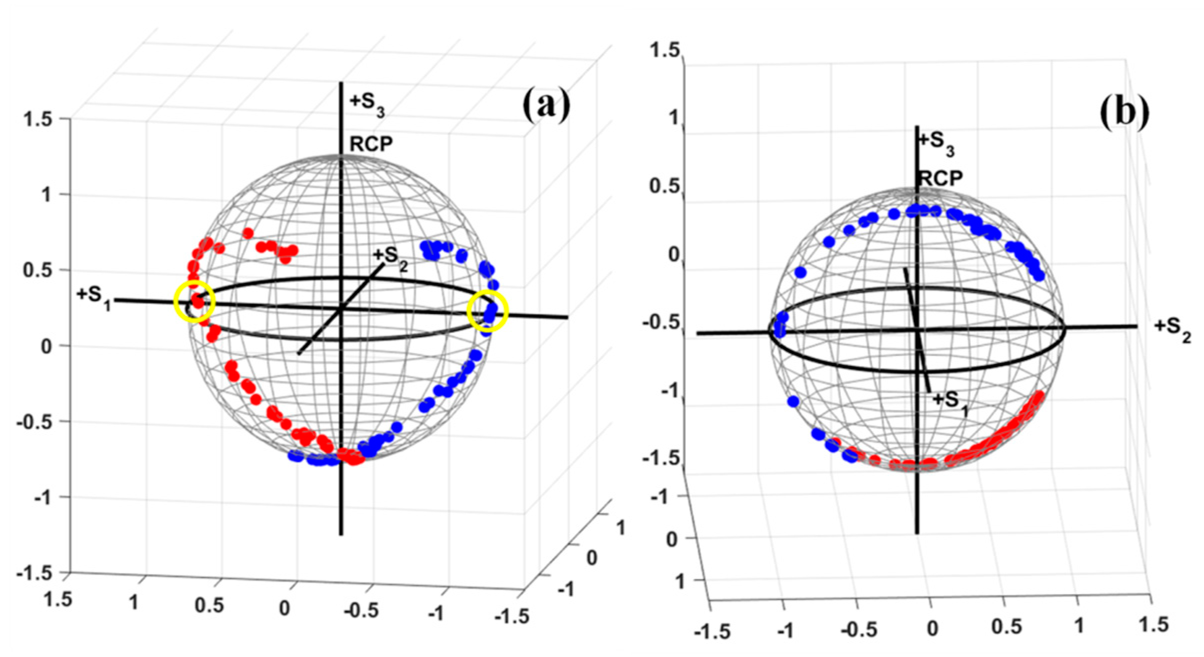
A comprehensive quantitative study of the SOP modulation of the SLM can provide more interesting information about its performance as a retarder. For this purpose, the polarization modulation characteristics of the SLM were further investigated by projecting the SOPs of the output light within the grayscale range of the SLM using the Poincare sphere. Figure 6a,b present the SOP modulation trajectories corresponding to ±45° polarized and xy-polarized incident light, respectively. The SOP modulations (trajectories) corresponding to the two orthogonal input SOPs are orthogonal to each other after reflecting from the SLM. It can be verified from Figure 6a,b that the corresponding SOP trajectories are mirror replicas (orthogonal) of each other. Further observations reveal that the SOP at grayscale 180 lies on the equator of the Poincare sphere (highlighted with yellow circles in Figure 6a), which validates our earlier results; that is, the input 45° polarized light is rotated into linearly polarized light at grayscale 180.
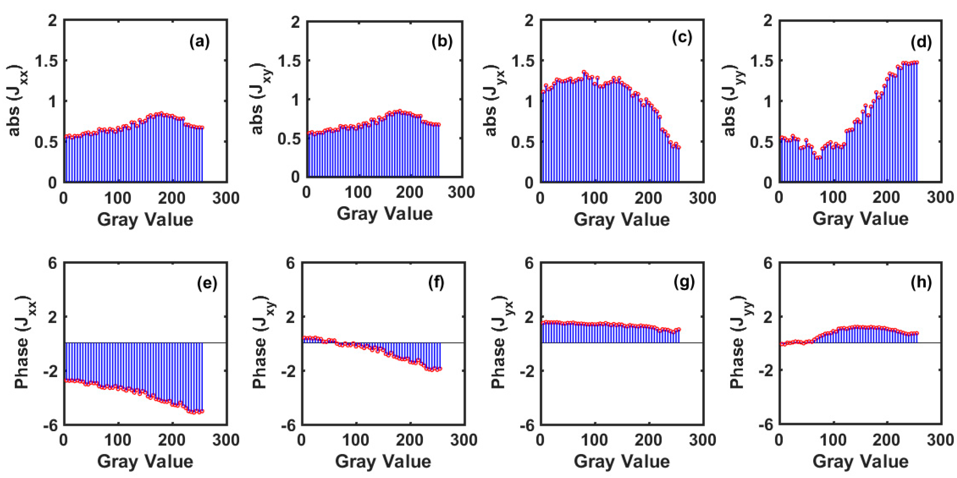
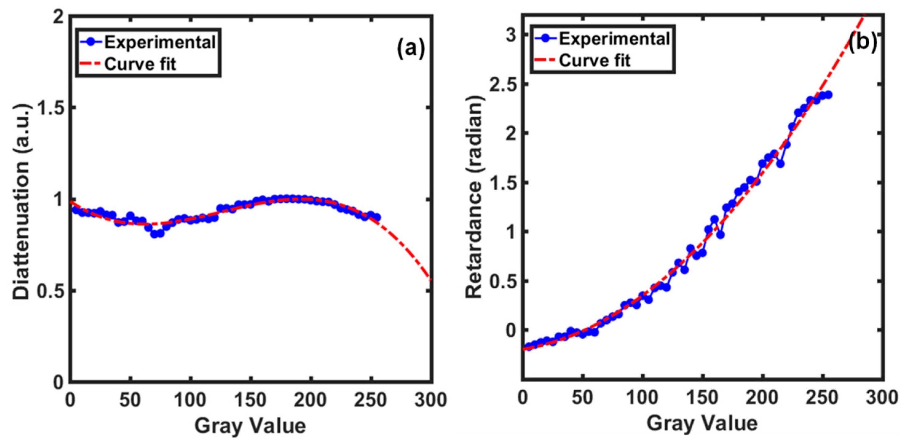
After characterizing the polarization modulation characteristics of the SLM, the Jones matrix components of the SLM were determined using Equation (7a–d). The corresponding amplitude and phase components were plotted against different grayscales of the SLM and are illustrated in Figure 7a–d and Figure 7e–h, respectively. Figure 7a–d show that the amplitude modulation corresponding to the first two Jones components, i.e., Jxx and Jxy, is similar (0.5–0.8) for various grayscales of the SLM, whereas a reverse trend is observed for the other two components (Jyx and Jyy). Similarly, the phase variation for the Jones matrix components implies that the SLM can modulate the phase of light within the range of 0 to π, depending on its different grayscales. Although the Jones matrix components do provide vital information about the amplitude and phase modulation characteristics of the SLM, crucial anisotropic polarization properties, i.e., diattenuation and retardance, cannot be determined directly from the Jones matrices. For this purpose, these properties were retrieved using polar decomposition of the Jones matrices of the SLM using Equations (9) and (10a,b). Figure 8a,b present the diattenuation and retardance of the SLM for its various grayscales. It is clear from Figure 8a that the SLM sustains its diattenuation property within its entire grayscale range. On the other hand, the retardance curve of the SLM indicates that the SLM provides a phase modulation of 0 to π (Figure 8b).
In general, the ideal curvature of the phase modulation curve of the SLM can be optimized using a polynomial function of grayscales [25]. In this study, the experimental curve for the anisotropic properties of the SLM is optimized with the third-order polynomial function and is represented with a red dotted curve in their corresponding figures.
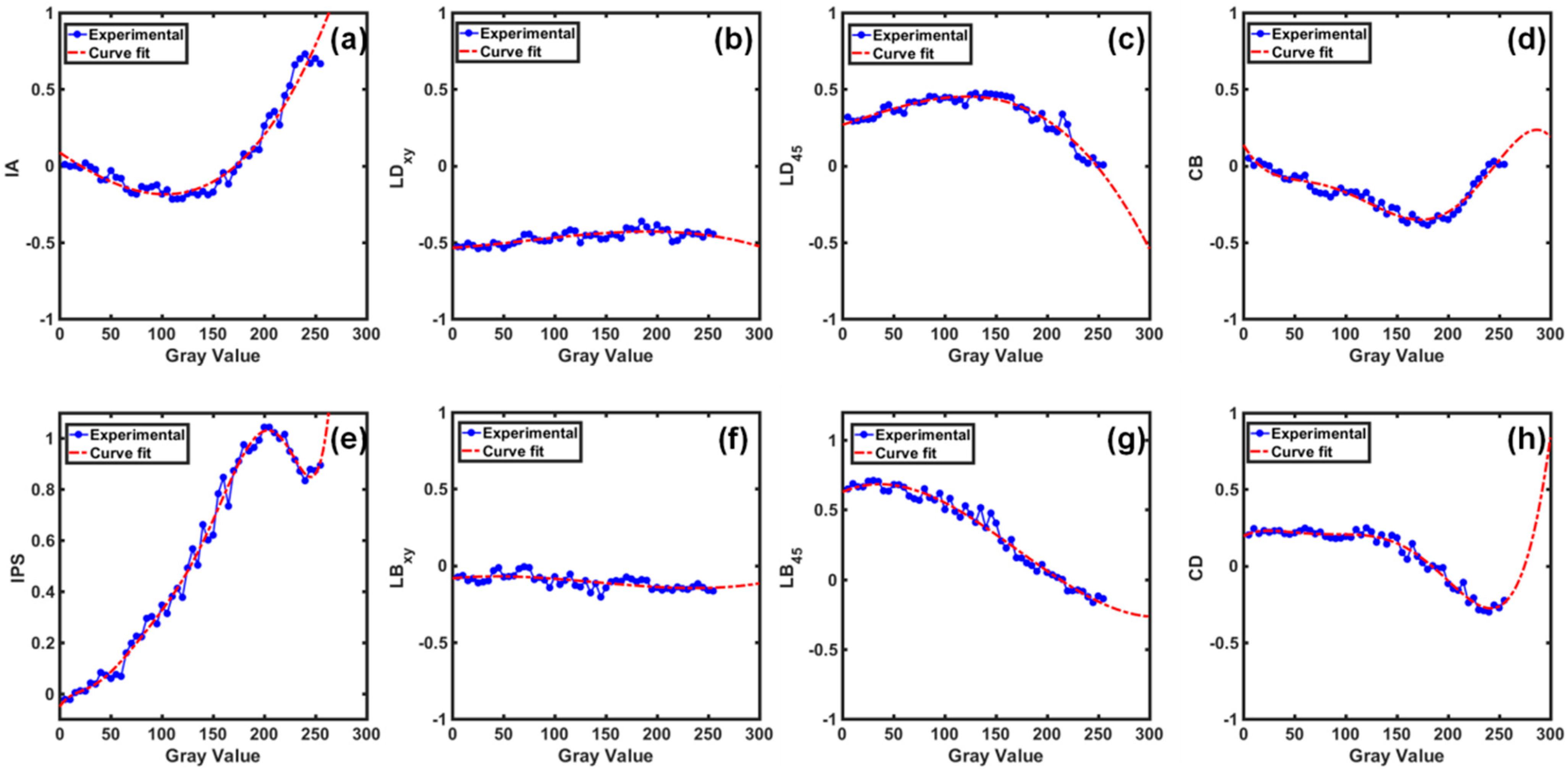
Direct retrieval of anisotropic properties (isotropic absorption (IA), isotropic phase shift (IPS), linear dichroism (LD), circular dichroism (CD) linear birefringence (LB), and circular birefringence (CB)) from measured Jones matrices were determined using a novel algebraic method of Jones matrix decomposition (see Equations (11)–(13)). Figure 9 presents the variation in the anisotropic properties of the SLM as a function of its grayscales. These anisotropic properties exhibit a significant variation within the grayscale range of the SLM. Figure 9a,e present that the SLM shows a monotonic trend for the IA and IPS, respectively. On the other hand, minor variation is observed for LDxy and LBxy for grayscales of the SLM (Figure 9b,f). This implies that LDxy and LBxy are independent of the applied pixel voltages, i.e., grayscales of the SLM. Similarly, a decreasing trend is observed for the anisotropic properties, viz., LD45, and LB45 (Figure 9c,g, respectively). Further, Figure 9d,h indicate that the CD and CB exhibit a similar trend for the grayscales of the SLM. Therefore, the SLM exhibits a anisotropic nature throughout its grayscale range. These anisotropic properties originate from the change in the relative orientation of LC molecules at different grayscales. The relative rotation of LC molecules leads to a change in the refractive index, and it yields fluctuations in anisotropic properties, e.g., birefringence and phase shifts.
5. Conclusions
In this paper, we experimentally demonstrate the complete polarimetric characterization of a TNLC-SLM for its entire grayscale range using the combined Jones-Stokes polarimetry. The amplitude, phase, and SOP modulation characteristics of the SLM are experimentally determined using a novel polarization-dependent interferometric experimental set-up, which is designed by combining Sagnac and Mach–Zehnder interferometers. The Jones matrix components are determined from the recorded interference patterns at various grayscales of the SLM using the FFA technique. Furthermore, the anisotropic response of the SLM is calibrated. The anisotropic properties of the SLM are retrieved from the measured Jones matrices using two decomposition methods, i.e., polar decomposition and an algebraic method for Jones matrix decomposition. This study provides a rapid and robust characterization of the essential anisotropic properties of the SLM viz., dichroism, birefringence, and isotropic absorption. The algebraic method for Jones matrix decomposition can be further utilized for the polarimetric characterization of other anisotropic birefringent samples (LC cells, biological samples, etc.), as well as for in-depth tissue imaging. The corresponding results indicate that the SLM (Holoeye, LC-R720) exhibits significant amplitude and phase modulation (0 to π) characteristics within its grayscale range. The SOP modulation characteristics of the SLM indicate that it can be utilized as an optical retarder and diattenuator by providing appropriate pixel voltage (grayscale) to the SLM. Despite these modulation characteristics, it also exhibits crucial variations for its anisotropic properties. The anisotropic properties along the xy axes are constant only for the grayscales of the SLM, whereas a decreasing trend is observed for the anisotropic characteristics along the 45° axis. This signifies that the SLM shows typically different anisotropic responses with respect to different reference axes. The polarimetric response of the SLM only fluctuates for applied pixel voltage, particularly at its mid-grayscale range. These fluctuations can originate due to the relative rotation of LC molecules depending on the different grayscales of the SLM. Other possible reasons might be manufacturing discrepancies (display curvature) and the limited fill factor of the SLM. In addition, undesired effects, e.g., phase flicker, might also be responsible for the fluctuations in polarimetric features of the SLM. In this study, phase flicker is not taken into account in the experimental procedure. Therefore, one could obtain improved SLM modulation features by circumventing the phase flicker effect. In brief, this study provides a complete polarimetric calibration of the SLM (Holoeye, LC-R 720). The proposed Jones decomposition methods can be utilized for rapid polarimetric measurements of anisotropic samples. The immediate applications of this study involve the utilization of the SLM in beam shaping, tissue polarimetry, and structured light applications.
Author Contributions
Conceptualization: V.T. and N.S.B.; methodology: V.T. and N.S.B., writing—original draft preparation: V.T.; review and editing: N.S.B.; supervision: N.S.B. All authors have read and agreed to the published version of the manuscript.
Funding
This research received no external funding.
Institutional Review Board Statement
Not applicable.
Informed Consent Statement
Not applicable.
Data Availability Statement
The datasets used and/or analyzed during the current study are available from the corresponding author on reasonable request.
Acknowledgments
V.T. would like to acknowledge DST-INSPIRE (IF-170861).
Conflicts of Interest
The authors declare no conflict of interest.
References
- Sturesson, C.; Nilsson, J.; Eriksson, S. Non-invasive imaging of microcirculation: A technology review. Med. Devices Évid. Res. 2014, 7, 445–452. [Google Scholar] [CrossRef] [Green Version]
- Prylepa, A.; Reitböck, C.; Cobet, M.; Jesacher, A.; Jin, X.; Adelung, R.; Schatzl-Linder, M.; Luckeneder, G.; Stellnberger, K.-H.; Steck, T.; et al. Material characterisation with methods of nonlinear optics. J. Phys. D Appl. Phys. 2018, 51, 043001. [Google Scholar] [CrossRef]
- Hall, S.A.; Hoyle, M.-A.; Post, J.S.; Hore, D.K. Combined Stokes Vector and Mueller Matrix Polarimetry for Materials Characterization. Anal. Chem. 2013, 85, 7613–7619. [Google Scholar] [CrossRef]
- Spandana, K.U.; Mahato, K.K.; Mazumder, N. Polarization-resolved Stokes-Mueller imaging: A review of technology and applications. Lasers Med. Sci. 2019, 34, 1283–1293. [Google Scholar] [CrossRef]
- Ghosh, N. Tissue polarimetry: Concepts, challenges, applications, and outlook. J. Biomed. Opt. 2011, 16, 110801. [Google Scholar] [CrossRef] [Green Version]
- Duran, V.; Lancis, J.; Tajahuerce, E.; Climent, V. Poincaré Sphere Method for Optimizing the Phase Modulation Response of a Twisted Nematic Liquid Crystal Display. J. Disp. Technol. 2007, 3, 9–14. [Google Scholar] [CrossRef]
- Xia, J.; Chang, C.; Chen, Z.; Zhu, Z.; Zeng, T.; Liang, P.-Y.; Ding, J. Pixel-addressable phase calibration of spatial light modulators: A common-path phase-shifting interferometric microscopy approach. J. Opt. 2017, 19, 125701. [Google Scholar] [CrossRef]
- Sarkadi, T.; Koppa, P. Measurement of the Jones matrix of liquid crystal displays using a common path interferometer. J. Opt. 2011, 13, 035404. [Google Scholar] [CrossRef]
- Tiwari, V.; Gautam, S.K.; Naik, D.N.; Singh, R.K.; Bisht, N.S. Characterization of a spatial light modulator using polarization-sensitive digital holography. Appl. Opt. 2020, 59, 2024–2030. [Google Scholar] [CrossRef]
- Chandra, A.D.; Banerjee, A. Rapid phase calibration of a spatial light modulator using novel phase masks and optimization of its efficiency using an iterative algorithm. J. Mod. Opt. 2020, 67, 628–637. [Google Scholar] [CrossRef]
- Tiwari, V.; Bisht, N.S. Statistical interpretation of Mueller matrix images of spatial light modulator. In Proceedings of the 2019 Workshop on Recent Advances in Photonics (WRAP), Guwahati, India, 13–14 December 2019. [Google Scholar]
- Oton, J.; Millán, M.S.; Ambs, P.; Cabre, E.P. Advances in LCoS SLM characterization for improved optical performance in image processing. In Proceedings of the Optical and Digital Image Processing; SPIE-The International Society for Optical Engineering: Washington, DC, USA, 2008; Volume 7000, p. 70001. [Google Scholar]
- Rosen, J.; Kelner, R.; Kashter, Y. Incoherent digital holography with phase-only spatial light modulators. J. Micro/Nanolithography MEMS MOEMS 2015, 14, 041307. [Google Scholar] [CrossRef] [Green Version]
- Márquez, A.; Moreno, I.; Iemmi, C.; Lizana, A.; Campos, J.; Yzuel, M. Mueller-Stokes characterization and optimization of a liquid crystal on silicon display showing depolarization. Opt. Express 2008, 16, 1669–1685. [Google Scholar] [CrossRef] [Green Version]
- Otón, J.M.; Oton, E.; Quintana, X.; Geday, M.A. Liquid-crystal phase-only devices. J. Mol. Liq. 2018, 267, 469–483. [Google Scholar] [CrossRef]
- Márquez, A. Characterization of edge effects in twisted nematic liquid crystal displays. Opt. Eng. 2000, 39, 3301. [Google Scholar] [CrossRef]
- Calderón-Hermosillo, Y.; García-Márquez, J.; Espinosa-Luna, R.; Ochoa, N.A.; López, V.; Aguilar, A.; Noé-Arias, E.; Alayli, Y. Flicker in a twisted nematic spatial light modulator. Opt. Lasers Eng. 2013, 51, 741–748. [Google Scholar] [CrossRef]
- Zheng, M.; Chen, S.; Liu, B.; Weng, Z.; Li, Z. Fast measurement of the phase flicker of a digitally addressable LCoS-SLM. Optik 2021, 242, 167270. [Google Scholar] [CrossRef]
- Veronica, C.; Elena, A.; Katkovnik, V.; Shevkunov, I.; Egiazarian, K. Pixel-Wise Calibration of the Spatial Light Modulator. In Frontiers in Optics/Laser Science; Paper JTu1B.31; Optical Society of America: Washington, DC, USA, 2020. [Google Scholar]
- Wolfe, J.E.; Chipman, R.A. Polarimetric characterization of liquid-crystal-on-silicon panels. Appl. Opt. 2006, 45, 1688–1703. [Google Scholar] [CrossRef]
- Demars, L.A.; Mikuła-Zdańkowska, M.; Falaggis, K.; Porras-Aguilar, R. Single-shot phase calibration of a spatial light modulator using geometric phase interferometry. Appl. Opt. 2020, 59, D125–D130. [Google Scholar] [CrossRef] [PubMed]
- Tiwari, V.; Pandey, Y.; Bisht, N.S. Spatially Addressable Polarimetric Calibration of Reflective-Type Spatial Light Modulator Using Mueller-Stokes Polarimetry. Front. Phys. 2021, 9, 400. [Google Scholar] [CrossRef]
- Durán, V.; Clemente, P.; Martínez-León, L.; Climent, V.; Lancis, J.; Martínez-León, L. Poincare-sphere representation of phase-mostly twisted nematic liquid crystal spatial light modulators. J. Opt. A Pure Appl. Opt. 2009, 11, 085403. [Google Scholar] [CrossRef]
- Kim, Y.; Jeong, J.; Jang, J.; Kim, M.W.; Park, Y. Polarization holographic microscopy for extracting spatio-temporally resolved Jones matrix. Opt. Express 2012, 20, 9948–9955. [Google Scholar] [CrossRef] [PubMed]
- Dai, Y.; Antonello, J.; Booth, M.J. Calibration of a phase-only spatial light modulator for both phase and retardance modulation. Opt. Express 2019, 27, 17912–17926. [Google Scholar] [CrossRef] [PubMed]
- Sreelal, M.M.; Vinu, R.V.; Singh, R.K. Jones matrix microscopy from a single-shot intensity measurement. Opt. Lett. 2017, 42, 5194. [Google Scholar] [CrossRef] [PubMed]
- Nee, S.-M.F. Decomposition of Jones and Mueller matrices in terms of four basic polarization responses. J. Opt. Soc. Am. A 2014, 31, 2518–2528. [Google Scholar] [CrossRef] [PubMed]
Figure 1.
Schematic of the relative rotation of TNLCs with respect to applied pixel voltage (grayscale) of the SLM (TNLC: twisted nematic liquid crystal, E: direction of the applied electric field).
Figure 1.
Schematic of the relative rotation of TNLCs with respect to applied pixel voltage (grayscale) of the SLM (TNLC: twisted nematic liquid crystal, E: direction of the applied electric field).

Figure 2.
Schematic of the polarization interferometer for Jones matrix imaging of SLM. HWP: half-wave plate, Ln (n = 1 to 5): lenses, SLM: spatial light modulator, BSn (n = 1 to 3): non-polarizing beam splitter, PBS: polarizing beam splitter, Mn (n = 1, 2): mirrors, CCD: charge-coupled device, BD: beam dump.

Figure 3.
(a) Schematic of the recorded hologram (I(x,y)), (b) recorded interference patterns (fringes) for (i–iii) +45° polarized and (iv–vi) −45° polarized input light at three grayscales of SLM (5, 180, and 255), respectively.
Figure 3.
(a) Schematic of the recorded hologram (I(x,y)), (b) recorded interference patterns (fringes) for (i–iii) +45° polarized and (iv–vi) −45° polarized input light at three grayscales of SLM (5, 180, and 255), respectively.

Figure 4.
Recorded interferogram and corresponding Fourier spectrum at grayscale 255 of the SLM +45° polarized input light. Asterisk (*) represents the conjugate of the corresponding field.
Figure 4.
Recorded interferogram and corresponding Fourier spectrum at grayscale 255 of the SLM +45° polarized input light. Asterisk (*) represents the conjugate of the corresponding field.

Figure 5.
Polarization modulation characteristics of the SLM within its grayscale range (0–255). (a) SPP variation (S1P, S2P, and S3P) for +45° polarized (b) SPP variation (S1m, S2m, and S3m) and for −45° polarized input light; (c) DOP variation for +45° polarized (blue plot) and −45° polarized (red plot) input light.

Figure 6.
Poincare sphere representation of SOP modulation characteristics of the SLM (a) for −45° polarized (red plot) and for −45° polarized (blue plot) input light, and (b) for x-polarized polarized (red plot) and y-polarized (blue plot) input light. Circles in yellow represent the SOP at grayscale 180.

Figure 7.
Jones matrix components as a function of grayscales of the SLM. (a–d) Amplitude and (e–h) phase of Jones matrix components. Amplitude is represented in arbitrary units and phase is represented in radians.
Figure 7.
Jones matrix components as a function of grayscales of the SLM. (a–d) Amplitude and (e–h) phase of Jones matrix components. Amplitude is represented in arbitrary units and phase is represented in radians.

Figure 8.
(a) Diattenuation and (b) retardance curves within grayscale range (0–255) of the SLM. Red dotted line represents the optimized curve fit (3rd-order polynomial) for the experimental data.
Figure 8.
(a) Diattenuation and (b) retardance curves within grayscale range (0–255) of the SLM. Red dotted line represents the optimized curve fit (3rd-order polynomial) for the experimental data.

Figure 9.
Anisotropic properties of the SLM as a function of its grayscales. (a) IA: isotropic absorption, (b) LDxy: linear dichroism along the xy axis, (c) LD45: linear dichroism along ±45 axes, (d) CB: circular birefringence, (e) IPS: isotropic phase shift, (f) LBxy: linear birefringence along the xy axis, (g) LB45: linear birefringence along ±45 axes, (h) CD: circular dichroism. Red dotted line represents the optimized curve fit for the experimental data.


Table 1.
Anisotropic properties using the algebraic method for Jones matrix decomposition.
| S. No. | Parameter | Anisotropic Properties of the Sample | |
|---|---|---|---|
| 1 | A | Real (A) | Isotropic absorption (IA) |
| Imaginary(A) | Isotropic phase shift (IPS) | ||
| 2 | B | Real (B) | Linear dichroism along xy axis (LDxy) |
| Imaginary (B) | Linear birefringence along xy axis (LBxy) | ||
| 3 | C | Real (C) | Linear dichroism along ±45 deg. axis (LD45) |
| Imaginary (C) | Linear birefringence along ±45 deg. axis (LB45) | ||
| 4 | D | Real (D) | Circular birefringence (CB) |
| Imaginary (D) | Circular dichroism (CD) | ||
Publisher’s Note: MDPI stays neutral with regard to jurisdictional claims in published maps and institutional affiliations. |
© 2022 by the authors. Licensee MDPI, Basel, Switzerland. This article is an open access article distributed under the terms and conditions of the Creative Commons Attribution (CC BY) license (https://creativecommons.org/licenses/by/4.0/).
Share and Cite
MDPI and ACS Style
Tiwari, V.; Bisht, N.S. Combined Jones–Stokes Polarimetry and Its Decomposition into Associated Anisotropic Characteristics of Spatial Light Modulator. Photonics 2022, 9, 195. https://doi.org/10.3390/photonics9030195
AMA Style
Tiwari V, Bisht NS. Combined Jones–Stokes Polarimetry and Its Decomposition into Associated Anisotropic Characteristics of Spatial Light Modulator. Photonics. 2022; 9(3):195. https://doi.org/10.3390/photonics9030195
Chicago/Turabian StyleTiwari, Vipin, and Nandan S. Bisht. 2022. "Combined Jones–Stokes Polarimetry and Its Decomposition into Associated Anisotropic Characteristics of Spatial Light Modulator" Photonics 9, no. 3: 195. https://doi.org/10.3390/photonics9030195
Note that from the first issue of 2016, this journal uses article numbers instead of page numbers. See further details here.