3D Volume Rendering of Invertebrates Using Light-Sheet Fluorescence Microscopy

Abstract

Light-Sheet Fluorescence Microscopy has recently emerged as the technique of choice for obtaining high quality three-dimensional (3D) images of whole organisms, with low photo-damage and fast acquisition rates. Unlike conventional optical and confocal microscopy or scanning electron microscopy systems, it offers the possibility of obtaining multiple views of the sample by rotating it. We show that the use of light-sheet fluorescence microscopy, for the analysis of invertebrates, provides a fair compromise compared to scanning electron microscopy in terms of resolution, but avoids some of its drawbacks, such as sample preparation or limited three-dimensional perspectives. In this paper, we will show how LSFM techniques can provide a cheap, high quality, multicolor, 3D alternative to classic microscopes, for the study of the morphological structure of insects and invertebrates in morphogenesis studies of the whole animal.

1. Introduction

Arthropods make up between 50 percent and 85 percent of the animals on the planet. Although some species, such as Drosophila melanogaster [1], are well known and extensively used as laboratory model organisms to generate new mutant strains, new species appear constantly and need to be characterized. In addition, due to globalization, new invasive species appear in locations where they have never been seen before. For these reasons, there is a need for imaging tools, for faster and accurate phenotyping of arthropods, able to generate 3D digital models, robust and precise enough to create physical models. Entomology research, featuring repetitive phenotypic analyses of insects (taxonomic, morphogenesis, quantitative genetics and mutant screens), will be greatly facilitated by such 3D imaging tools.

Nowadays, entomology mainly uses three techniques: photography combined with focus stacking, scanning electron microcopy and confocal microscopy. Photography, combined with focus stacking, is a cheap and simple solution that requires only a camera and specific software to produce good-quality images. However, it does not allow one to create 3D models. Scanning Electron Microscopy (SEM) provides high-quality images, with the best resolution possible of up to nm range [2]. However, it is expensive (EUR ~200,000) and requires complex sample preparation procedures. Moreover, it only provides restricted views, although it is possible to tilt the sample to obtain stereo photographs [3]. The sample should, therefore, be correctly oriented to image a desired morphological feature. The only way to create 3D models is through cryosections, leading to a tedious sample preparation [4]. Moreover, insect specimens with hairs, spines, and other projections are particularly prone to charging, even at low accelerating voltages, producing charging lines of streaks at the final image. In the middle, we find confocal microscopy, providing good-quality images from exoskeleton auto-fluorescence [5]. Although it allows the creation of 3D models, this is a complex and time-consuming task, limited to a single view. Moreover, is could also be quite expensive (EUR ~300,000).

Light-Sheet Fluorescence Microscopy (LSFM) [6], such as Selective Plane Illumination Microscopy (SPIM) [7] or Digital Scanned Laser light-sheet Microscopy (DSLM) [8], may represent an alternative to the methods described above. LSFM offers the high speeds, large fields of view and long-term imaging capacity needed to image whole cells, tissues and organisms, at high resolution. The operation principle, as confocal, is based on fluorescence. Although with wild-type arthropods, the signal only comes from auto-fluorescence, multicolor imaging allows one to obtain relevant morphological information and, if needed, enables specific labelling with fluorescent dyes or genetically encoded proteins. The difference with confocal is that in LSFM, the illumination is done perpendicularly to the detection. The illumination laser beam is shaped into a rectangular cross-section and then focused to a thin “sheet of light”, using a cylindrical lens (SPIM) or a fast laser scanner (DSLM) in the focal plane of the detection objective. As the sample is moved through the focal plane, different planes of the sample are illuminated, creating a z stack of images that can be three-dimensionally reconstructed. Compare with confocal, since only the portion of the sample being imaged is illuminated, it provides reduced photo-bleaching and photo-damage, ensuring long-term sample viability for live imaging experiments, especially in DSLM setups [9]. As the light-sheet thickness can be tailored to the micron range, it achieves good sectioning of the sample and out-of-focus light suppression. The lateral resolution is given by the detection objective only.

Compared with SEM and confocal microscopy, LSFM performs best using a fast, high-sensitivity acquisition, based on sCMOS or CCD cameras, and can be implemented at a less expensive overall cost (EUR ~20,000). It does not require complex sample preparation as SEM does, and provides reasonable isotropic resolution for phenotyping and anthropoid classification. Among the advantages of LSFM, probably the most important is the possibility of recording multi-views of the sample by rotating it and, using fusion algorithms [10], to obtain 3D volume renderings. This feature leads to the possibility of acquiring a detailed three-dimensional volume reconstruction of the sample, not achievable with any other microscopic technique. The main drawbacks are shadowing effects due to sample absorption in single-side illumination setups (which can be partially solved with two-sided [11] or multi-view recording [12]) and the large amount of data generated.

Since LSFM provides optical sectioning, even with lenses that have a large working distance and a relatively low numerical aperture, it is especially well suited for the investigation of the morphology of large samples. We have already successfully used LSFM to image different biological models, including zebrafish (Danio rerio) [13], Caenorhabditis elegans nematodes [14], Drosophila melanogaster fly and Arabidopsis thaliana plant [15], among others. In the present paper, we will show how LSFM techniques could provide a cheap, low-resolution alternative to scanning electron and confocal microscopes for the study of the complete morphological structure of insects and other invertebrates. These techniques open the possibility to create full 3D digital models of invertebrates for the study of these organisms in the digital world, to export them to virtual reality scenarios and to make it easier for entomologists to share their discoveries.

2. Materials and Methods

2.1. Experimental Set-Up

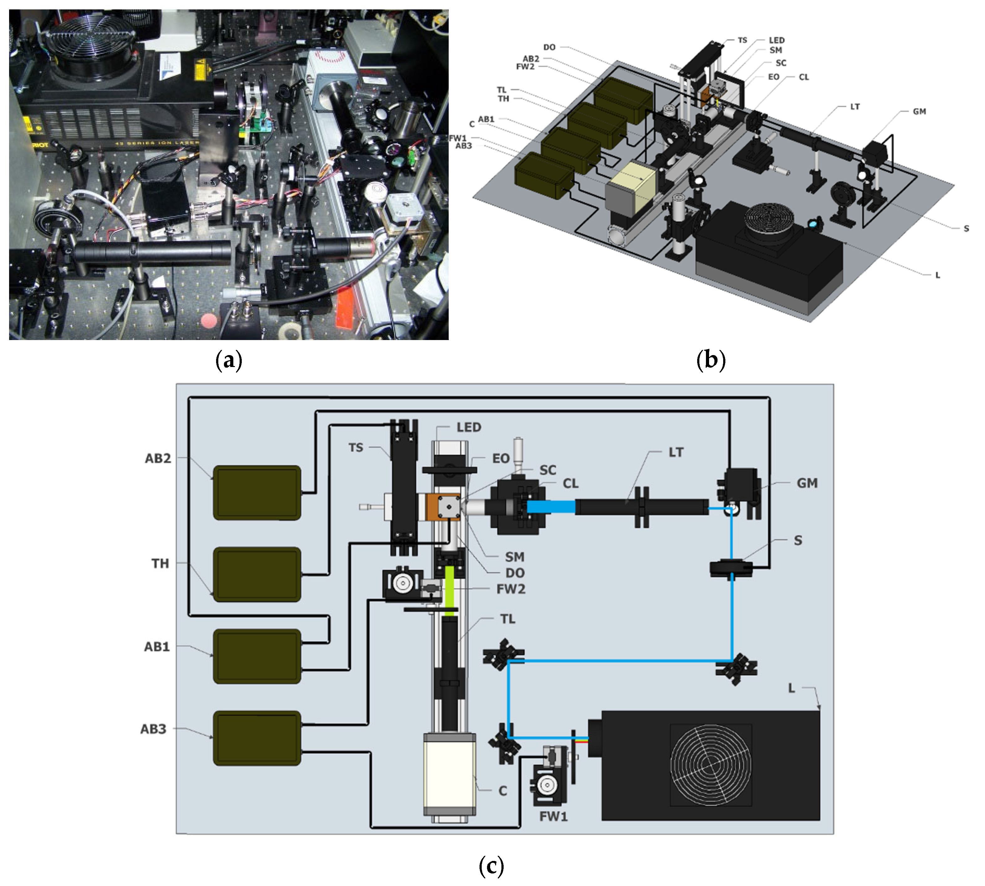
All the images shown in this paper were acquired with a homemade Light-Sheet Fluorescence Microscopy system, based on an open software (Micro-manager) [16] and hardware (Arduino) approach, the OpenSpinMicroscopy project [17]. A description of the setup can be found in Figure 1. Full descriptions of the apparatus, as well as source code of the acquisition software and instructions to build it are available through our webpage (https://sites.google.com/site/openspinmicroscopy/ (accessed on 1 February 2022)).

The optical setup is shown in Figure 1. Sample illumination is performed with an Argon/Kryton laser (Melles Griot 35 LTL 835–230) providing excitation wavelengths of 488 nm, 568 nm and 647 (L). The different excitation laser lines are selected using a filter wheel (FW1) with four different filters (D488/10, 568/10, 488/568DBX and D647/10). A shutter (Uniblitz electronics LS3T2) is used to block the laser beam (S) and a varying neutral density filter is used control the light dosage applied to the sample.

In order to create the light sheet on the sample plane we implemented the DSLM modality, with a single galvanometric mirror (6210H Cambridge technologies) scanning the laser beam in the vertical axis (GM). The optical plane of the galvo is conjugated with the back focal aperture of an objective lens (Nikon Plan Fluor 4x; NA: 0.13; WD: 17.4 mm) using a 3.5x telescope system (LT) consisting of 50 mm and 180 mm achromatic doublet lenses (Thorlabs). Alternatively, SPIM mode can be implanted by inserting a 50 mm cylindrical lens (CL) between the 175 mm lens and the excitation objective in such a way that the vertical axis of the beam is focused on the back aperture of the objective, while the horizontal axis fills the aperture.

For detection, air objectives (Nikon Plan Fluor 4x; NA: 0.13; WD: 17.4 mm or Plan Fluor 10x; NA: 0.3; WD: 16.7 mm) or a water immersion objective (Nikon LWD 16x; NA: 0.8 WD: 3 mm), placed perpendicularly to the excitation plane, are used to collect fluorescence emission. Excitation light is rejected using emission filters placed in the infinity space before the camera, with filters mounted in a second automatic filter wheel (FW2), consisting of the following: ET 480/40m-2p, HQ 535/70m-2p, HQ 580/25m-2p, HQ 620/90m-2p and HQ 640/25m-2p. Finally a 200 mm tube lens (TL) creates the image on the chip of a sCMOS camera (Hamamatsu Orca-Flash4) recording the entire illuminated plane at the same time (C). Using the 4x we achieve a field of view (FoV) of 3.3 mm × 3.3 mm while the 10x provides 1.33 mm × 1.33 mm FoV, with 1.61 µm and 0.65 µm pixel size, respectively. The 16x objective provides a total field of view of 819 µm × 819 µm with 0.4 µm pixel size.

Different planes are collected by moving the sample using a linear DC motor (Thorlabs MTS50A-Z8 with servo controller TDC001) through the light sheet (TS), with a step size of 2–3 µm. This allows us to obtain a typical z-stack of around 220 images (2048 × 2048 pixels) covering the whole specimen in a relatively short period of time (20 to 30 s). We normally used an integration time of 100 ms, which in theory provides 10 frames per second (fps). However, motor movement’s delay limits real scanning speed to 7–8 fps. In order to avoid the deleterious effect of light absorption from the sample and the shadowing effects our system is able to obtain multi-view images of the sample by rotating the sample with a stepper motor (Astrosyn 9598642) (SM). This easy and cheap solution allows down to 1.8 degree steps and it is controlled with an Arduino UNO board (AB). Sample centering (X/Y axis) on the field of view of the camera is performed manually with two linear translation stages. Two more Arduino boards control the filter wheels and the galvanometric mirror, respectively.

2.2. Sample Preparation

All the samples used in this work are wild-type species, collected directly from the laboratory surroundings (ants, Tineola Bisselliella moth, Acyrthosiphon pisum aphid, Salticus scenicus spider and Daphnia pulex), or provided by our collaborators (Tetranychus urticae mite, Oecophylla smaragdina ant and Bicyclus anynana butterfly) and weren’t subjected to any further treatment. All of them (except Bicyclus anynana butterfly and Daphnia pulex) were euthanized by immersion in ethanol prior to imaging. Female Anopheles stephensi mosquitoes were reared and maintained (28 °C; 70–80% humidity under 12 h/12 h light/dark cycle) as described before [18]. Next, 3 to 4-day-old female mosquitoes were fed on BALB/c mice that were infected with Plasmodium berghei ANKA expressing GFP under the EEF1α promoter for 1 h following the assessment of gametocyte-stage parasites capable of exflagellation in fresh blood preparations and were maintained at 26 °C. Mosquitoes were used for imaging 18 days post-infection.

2.3. Sample Mounting

A key component on an LSFM microscope is sample mounting. Samples are placed on pipetting tips, embedded in low-melting-point agarose (0.5 to 1% concentrations), and submerged in a water-filled chamber (SC) to reduce optical aberrations. In order to perform multi-view fusion, 0.5 µm fluorescence beads (TetraSpeck, Invitrogen, Waltham, MA, USA) were diluted (1:10,000) and added to the agarose [10]. The other end of the plastic pipette is inserted on the rotational stepper motor (SM) for sample rotation, which is attached to a linear DC motor for sample scanning though the light sheet, as described in [17].

2.4. Image Processing

Image processing on the LSFM data was performed using Java open-source software Fiji [19]. Basic functions used include multicolor merging and maximum projection of 3D stacks. For multi-view fusion we used the “SPIM Registration” Fiji plugin [10], which extracts the three-dimensional position of fluorescent beads mixed within the low-melting-point agarose, finds correspondences between views, and finally merges all the views in a single 3D stack. Removal of the imaged beads from the final 3D stack was performed manually. When needed, stitching of different parts of the animals was performed by concatenating 3D stacks using the “Pairwise Stitching” Fiji plugin [20]. Volume renderings were performed using the “3D Viewer” Fiji plugin [21]. For image processing we used the same workstation that was used for acquisition, with an Intel Core i7 and 32 GB of RAM.

3. Results

One advantage of LSFM, compared to confocal and electron microscopy, is the possibility to 3D image whole animals in toto, such as the spider shown in Figure 2, from the family Saltidae (Salticus scenicus), in a considerably reduced amount of time and without complex sample preparations. To obtain fully volumetric reconstructions, several datasets (normally eight views recorded with 45° sample rotation) from different body segments need to be acquired and stitched (Figure S1). Afterwards they are fused into a single dataset (Figure 2a) using, as reference, the fluorescent beads embedded in the agarose block supporting the sample (Video S1).

LSFM also offers the possibility of obtaining high-resolution volumetric images of specific areas of interest by replacing the detection objective (DO). In this example, we zoomed into a pedipalp (Figure 2b,c) and the interstitial zone between the mid-body articulations (Figure 2d,e).

The technique presented here can be applied to several “hot”research fields, such as malaria disease, plants’ plagues, biodiversity characterization or water quality control, to name a few examples. In the following sections, we will display what LSFM may offer in terms of the volumetric imaging of different invertebrate species. Different possible applications of LSFM to entomology studies are: plasmodium infection of Anopheles mosquitoes in malaria studies (Figure 3); characterization of different individuals of mite species Tetranychus urticae (Figure 4); morphological comparison between different ant species (Figure 5); visualization of different time-points of the reproductive process on Daphnia pulex (Figure 6). Other examples, such as an Acyrthosiphon pisum aphid, a Tineola Bisselliella moth head (Figure S2), arthropod wing phenotyping (Figure S3), and eyespot formation in Bicyclus anynana butterfly wings (Figure S4), can be found in the Supplementary Materials.

3.1. LSFM Applied to Malaria Studies

Female Anopheles stephensi mosquitoes are responsible for malaria infection, one of the most deadly diseases in the world, due to transmission to humans of the protozoon Plasmodium. Developed within the mosquito, its cycle is very complex and not yet fully understood. Using LSFM, we are able to observe the overall morphology of this mosquito (see Figure 3a), obtaining high-resolution 3D volume renderings (Video S2). Besides morphological characterization of the mosquito, the infection process can also be studied by using GFP expressing sporozoites of Plasmodium berghei [22], shown in red in the figure. Under natural infection conditions, the ookinete (the developmental stage of the malaria parasite that invades the mosquito midgut) rests between the midgut epithelium and the luminal side of the basement membrane of the infected mosquito (Figure 3b). Sporozoites differentiate and develop in the midgut for 10–14 days. After this period, hundreds of sporozoites are released into the mosquito hemolymph and some are carried to the salivary glands. In Figure 3c,d it can be observed that a significant amount of sporozoites invade the salivary glands. Moreover, sporozoites can also be observed in the cavities of secretory cells at the distal end of the glands and, for the first time, we show that different parts of the arthropod, such as the legs, were also infected with Plasmodium sporozoites (Figure 3e,f).

Figure 3. Maximum intensity projection of the auto-fluorescence from Anopheles stephensi mosquitoes. (a) Whole mosquito anatomy. This image consists of the stitching of two 3D stacks obtained with a 4x objective, 488 nm laser illumination and long pass filter. See also Video S2. (b) Mosquito’s midgut region, imaged at 4x with two channels (GFP in red, auto-fluorescence in green). Specific regions were imaged at higher resolution with a 10x objective: (c) salivary gland; (d) GFP signal in the salivary gland indicating a high concentration of sporozoites; (e) head and (f) front legs. Sporozoites appear in in red. Scale bar: 100 µm.

Figure 3. Maximum intensity projection of the auto-fluorescence from Anopheles stephensi mosquitoes. (a) Whole mosquito anatomy. This image consists of the stitching of two 3D stacks obtained with a 4x objective, 488 nm laser illumination and long pass filter. See also Video S2. (b) Mosquito’s midgut region, imaged at 4x with two channels (GFP in red, auto-fluorescence in green). Specific regions were imaged at higher resolution with a 10x objective: (c) salivary gland; (d) GFP signal in the salivary gland indicating a high concentration of sporozoites; (e) head and (f) front legs. Sporozoites appear in in red. Scale bar: 100 µm.

3.2. LSFM for Characterization of Mites and Other Pest Species

Tetranychus urticae spider mite is a major pest of several crops, causing severe damage throughout the world [23]. Its genome was fully sequenced in 2011, being the first genome sequence from any chelicerate [24]. For this reason, is interesting to understand its biology, with the goal of preventing its deleterious effects on crops. We performed three-channel in toto LSFM imaging of virgin and mated females and males, in order to distinguish relevant morphological differences. The upper row of Figure 4 corresponds to the ventral side, while the lower row shows the dorsal area. Three-dimensional stacks were obtained using a 16x objective and three laser lines for illumination: 488 nm (red), 567 nm (green) and 647 nm (blue). In general, we observe a higher auto-fluorescence in the red/green channels, in mouth and legs tips. The strong sexual dimorphism can be appreciated, with the females bigger and more roundish than males (see Figure 4a,d), for which their legs appear larger compared with their bodies. In both cases, inside the animals, we observe the blue channel inner balls, distributed on both sides of the thorax, which may correspond to food. The sexual organs can be clearly distinguished by a higher auto-fluorescence in the red/green channels, especially the female gonads. Mated females (Figure 4c,f) present a higher fluorescence inside the ventral part, compared with virgin females (Figure 4b,e). A full 3D volume render can be found in Video S3. Another pest species affecting crops is Acyrthosiphon pisum aphid, displayed in Figure S2c,d and Video S4.

Figure 4. Maximum intensity projections from three different adult individuals of the spider mite species Tetranychus urticae. Two views are displayed: (a–c) ventral; (d–f) dorsal. The sexual dimorphisms can be observed between males (a,d), and females (b,c,e,f). Levels of auto-fluorescence inside the mite also change between mated (f) and virgin females (e) (see arrow). Images obtained using a 16x objective and three laser lines for illumination: 488 nm (red), 567 nm (green) and 647 nm (blue). Volume reconstructions can be found in Video S3. Scale bar: 100 µm.

Figure 4. Maximum intensity projections from three different adult individuals of the spider mite species Tetranychus urticae. Two views are displayed: (a–c) ventral; (d–f) dorsal. The sexual dimorphisms can be observed between males (a,d), and females (b,c,e,f). Levels of auto-fluorescence inside the mite also change between mated (f) and virgin females (e) (see arrow). Images obtained using a 16x objective and three laser lines for illumination: 488 nm (red), 567 nm (green) and 647 nm (blue). Volume reconstructions can be found in Video S3. Scale bar: 100 µm.

3.3. LSFM for Morphology Comparison between Different Ant Species

Ants are important components of ecosystems, not only because they constitute a great part of the animal biomass, but also because they act as ecosystem engineers [25]. Ant biodiversity is incredibly high [26], so proper methods to analyze ants’ morphological diversity may help entomologists in their routine work. In this work, we have imaged three different species: an arboreal ant, mainly found in Asia and Australia, Oecophylla smaragdina (Banks, 1768), donated by Roberto Keller, and two different undefined specimens, found in the laboratory surroundings (Figure 5 and Figure S2a,b).

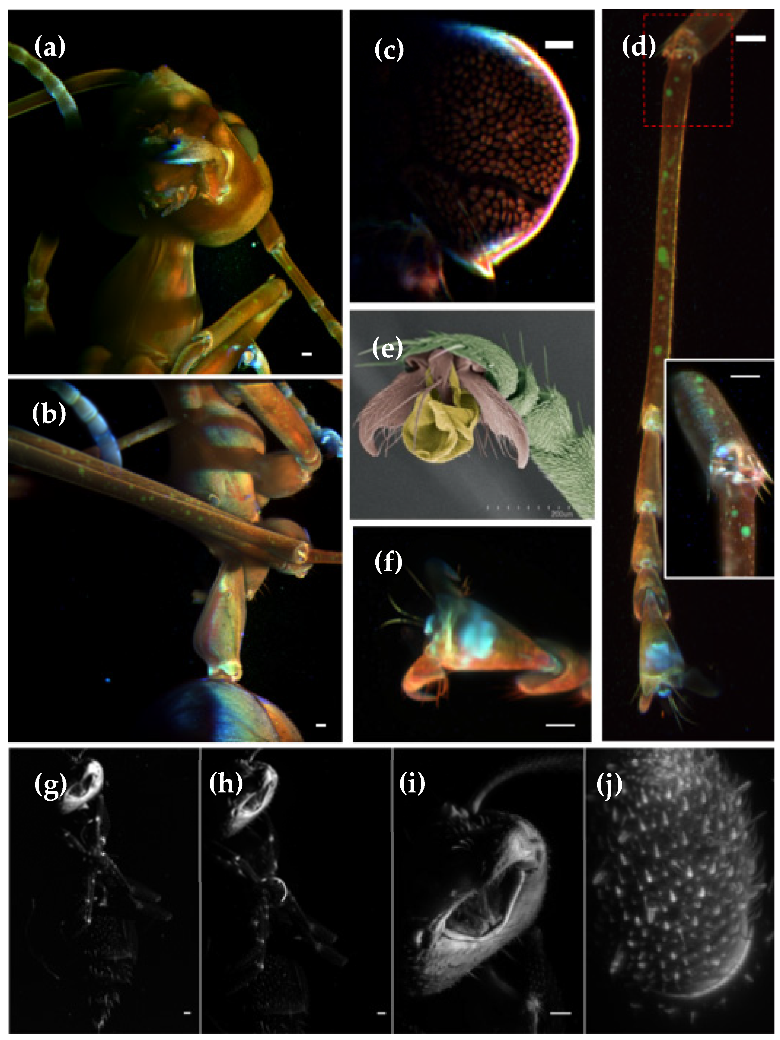
For the adult Oecophylla smaragdina ant, a maximum projection from the head, obtained from a single view, using a 4x detection objective, is presented in Figure 5a, while the mid-body is displayed in Figure 5b. We imaged this ant using three laser lines: 488 nm (red), 568 nm (green) and 647 nm (blue). As can be appreciated, strong auto-fluorescence in the blue channel is observed in the antennas and claws. Moreover, the legs present some pigmentation on the green channel. Its body is reddish and slightly transparent, allowing observation of several inner anatomical features, such as the brain structure (Figure 5c) and musculature. One of the ant’s legs, shown in Figure 5d, was removed and independently imaged at higher resolution, with a 16x objective (detail of the knee at inset image). A high-resolution image of the claw is depicted in Figure 5f. For the sake of comparison, we also present an SEM image from the claw, recorded on another specimen, Figure 5e. In Figure 5g–j, we present an unidentified ant, imaged using 488 nm laser illumination and different objective magnifications, i.e., 4x (NA 0.13), 10x (NA 0.1), 16x (NA 0.8) and 60x (NA 1). Those objectives provide 2.12, 0.92, 0.34 and 0.25 μm theoretical lateral resolution, respectively. Due to the short working distance of the 60x objective, only the tip of the antenna was imaged.

Figure 5. Maximum intensity projection of the auto-fluorescence from two different ant species. For Oecophylla smaragdina we imaged the (a) head and (b) the mid-body areas, using a 4x objective. Color images were obtained from three laser line illuminations: 488 nm (red), 568 nm (green) and 647 nm (blue). 3D volume renderings can be found in Video S5. (c) Single slice of the inner structure of the ant’s brain. (d) Ant leg imaged with higher resolution through a 16x objective, with the inset showing a zoom into the articulation region. (e) SEM image of an Oecophylla smaragdina claw. (f) Maximum intensity projection of a claw imaged using a 16x objective. Unidentified ant imaged with different objective magnifications (g) 4x, (h) 10x, (i) 16x and (j) 60x. In all cases we used a 488 nm laser illumination. Scale bar: 100 μm.

Figure 5. Maximum intensity projection of the auto-fluorescence from two different ant species. For Oecophylla smaragdina we imaged the (a) head and (b) the mid-body areas, using a 4x objective. Color images were obtained from three laser line illuminations: 488 nm (red), 568 nm (green) and 647 nm (blue). 3D volume renderings can be found in Video S5. (c) Single slice of the inner structure of the ant’s brain. (d) Ant leg imaged with higher resolution through a 16x objective, with the inset showing a zoom into the articulation region. (e) SEM image of an Oecophylla smaragdina claw. (f) Maximum intensity projection of a claw imaged using a 16x objective. Unidentified ant imaged with different objective magnifications (g) 4x, (h) 10x, (i) 16x and (j) 60x. In all cases we used a 488 nm laser illumination. Scale bar: 100 μm.

3.4. LSMF Applied to Aquatic Organisms: Daphnia Pulex

The technique described in this paper can also be extended to aquatic organisms, such as small crustaceans. Daphnia, popularly known as water fleas, live in fresh water, such as ponds, lakes and streams. Daphnia are excellent organisms for bioassays because they are highly sensitive to changes in water chemistry and inexpensive to raise in an aquarium [27].

Daphnia pulex is an extremely transparent fresh-water organism, ideal for microscopic imaging. An example is shown in Figure 6a, where it is possible to observe all the inner organs in the auto-fluorescence maximum intensity projection (see also Video S6). Their reproductive cycle can follow two different pathways, alternating between parthenogenetic (asexual) reproduction and sexual reproduction. Parthenogenetic reproduction is produced by “resting eggs”, created on each side of the dorsal part. Its epithelium, rich in keratin, presents an increased auto-fluorescence, as shown in the eight-view fusion in Figure 6b. During sexual reproduction, cycle eggs are formed inside the female, as shown in the cross-section in Figure 6c. Using two different laser lines (488 nm (red) and 568 nm (green)), we can clearly distinguish between the outer Daphnia membrane and embryo cells (red channel) and the egg cell walls (green channel). In Figure 6d, juvenile Daphnias can be observed inside the brood pouch of an adult female. These animals have gained interest as indicators for water quality control, since they are sensitive to toxins and prone to be colonized by other organisms, as shown in Figure 6e.

Figure 6. Auto-fluorescence from Daphnia pulex (a) maximum intensity projection obtained with 16x detection objective and 488 nm laser excitation. The inner organs are visible. A 3D volume rendering as well as the inner organs are shown in Video S6. (b) Volume reconstruction of a water flea that presents resting eggs in the dorsal part of its cuticle. (c) Cross-section of a daphnia with internal eggs. Auto-fluorescence excited with 488 nm appears in red and with 568 nm in green. (d) Cross-section of a daphnia with juveniles hidden inside its mother. (e) Cross-section of a daphnia with internal eggs, colonized by parasites (bright orange signal). Scale bar: 100 μm.

Figure 6. Auto-fluorescence from Daphnia pulex (a) maximum intensity projection obtained with 16x detection objective and 488 nm laser excitation. The inner organs are visible. A 3D volume rendering as well as the inner organs are shown in Video S6. (b) Volume reconstruction of a water flea that presents resting eggs in the dorsal part of its cuticle. (c) Cross-section of a daphnia with internal eggs. Auto-fluorescence excited with 488 nm appears in red and with 568 nm in green. (d) Cross-section of a daphnia with juveniles hidden inside its mother. (e) Cross-section of a daphnia with internal eggs, colonized by parasites (bright orange signal). Scale bar: 100 μm.

In conclusion, throughout the results section, we have provided several examples of what LSFM may offer, in terms of resolution, contrast, and penetration depth, for the complete three-dimensional morphological characterization of a variety of invertebrate species of special interest, for the study of malaria disease, plants’ plagues, biodiversity characterization or water quality control.

4. Discussion

Entomology studies are generally interested in phenotyping different arthropod species, in order to understand divergences in a population, changes during its developmental cycle, responses to changes in its ambient, environmental quality, or the effect of parasites and diseases. Traditionally, such studies have been performed using scanning electron microscopy, and to some extent, the use of fluorescence, through confocal microscopy.

Light-Sheet Fluorescence Microscopy (LSFM) has recently emerged as the technique of choice for obtaining high quality 3D images of whole organisms, with low photo-damage and fast acquisition rates. Here, we show that the use of LSFM, for the analysis of invertebrates, provides a fair compromise compared to scanning electron microscopy in terms of resolution, but avoiding some its drawbacks, such as sample preparation or limited three-dimensional perspectives. In our system, samples did not require any preparation, simply being held in their native state on the sample holder. In addition, unlike conventional optical or scanning electron microscopy systems, our LSFM approach offers the possibility of obtaining multi-views of the sample by rotating it.

The main source of auto-fluorescence in arthropods is chitin, the principal constituent of the exoskeleton, and allows reconstruction of the body shape with great detail. Purified chitin molecules show a maximum excitation at 450–460 [28] and maximum emission at 520 nm [29]. Other pigments present on the specimen surface, or even internally, if the sample is transparent enough, can be excited/collected with different laser lines and filter combinations, providing additional information of its anatomy. In our case, we have primarily used a 488 nm laser for chitin, and additional 568 nm and 647 nm lines for other pigments. Other lines, such as a 405 laser, would also contribute to enhancing the recorded auto-fluorescence information. In any case, the dependence on the auto-fluorescence signal to recover structural information represents the major drawback of this approach, compared with electron microscopy. We have noticed that areas lacking any fluorescent molecule may appear void in the volume rendering, as in the lateral part of the spider sample, although this never happened in the other arthropods imaged.

Unlike electron microscopy, LSFM (and sometimes confocal microscopy) provides the possibility to obtain information about the internal anatomy of the specimen in most of the samples shown in this article (i.e., mosquito, mite, daphnia and Oecophylla smaragdina ant). This is due, on one hand, to the partial transparency of the samples and, on the other hand, to the increased quantum efficiency offered by the sCMOS cameras used in LSFM, compared with PMTs used in confocal microscopy, thus, allowing the recording of even extremely low levels of signals. However, in most of the cases, penetration is compromised by scattering in non-transparent samples. During recent years, many tissue clearing methods have been developed and applied to the study of arthropods [30,31,32,33]. Those techniques consist of the homogenization of the sample refractive index, thus, reducing light scattering effects. The different types of clarification methods are divided into techniques based on tissue dehydration and solvent-based clearing (BABB, 3DISCO, iDISCO, etc.), and aqueous-based techniques (Scale/A, Clarity, CUBIC, etc.). However, a major problem is that solvent-based clearing can lead to tissue shrinkage, due to dehydration, while aqueous-based techniques normally produce tissue swelling. The method used in this paper allows one to obtain the real dimensions of the general anatomy, without this kind of shape distortion, and could be applied to physio-mechanical studies.

The major advantage of LSFM for the study of insects’ anatomy is the possibility to obtain fully volumetric reconstructions of the specimen. This is due to the microscope’s architecture, with its orthogonal illumination-detection scheme, and the sample mounting procedure, embedded in agarose and suspended between the objectives. For these reasons, samples can be freely rotated, providing different views that can be computationally fused into a single dataset. In addition, this configuration opens the door to combine LSFM data with other compatible techniques, such as Optical Projection Tomography (OPT) [17,34,35], providing low-resolution, but isotropic, information. The 3D models obtained can also be used for creating virtual reality scenarios, holograms, as well as full color 3D printing models [36], as shown in Figure S5 and Videos S7 and S8. Our approach is very powerful for outreach and education, as well as research, allowing a true 3D dimensional interaction with the experimental results. On the contrary, both confocal and electron microscopy are restricted to a single view.

Finally, but no less important, during recent years, this technology has become a cheap alternative to high-end commercial microscopes, thanks to several open-source initiatives, such as OpenSPIM [37], OpenSpinMicroscopy [17], Legolish [38], or other 3D-printed approaches [39]. These platforms allow not only the democratization of this technology, but also for the fostering of its adoption for non-experienced laboratories. In general, the cost of a basic LSFM system, as the one presented here, is at least an order of magnitude lower than confocal and electron microscopes.

In conclusion, here, we present LSFM as a cheap and affordable alternative to electron and confocal microscopy for invertebrate morphology characterization. We have shown the vast ensemble of possibilities that LSFM imaging offers for the study of non-manipulated arthropods, by means of their auto-fluorescence signal. In addition, the main attraction of LSFM is the possibility to obtain fully volumetric reconstruction of the specimen of interest, which could be used for several applications, from outreach to physio-mechanical studies.

References

- Roberts, D.B. Drosophila melanogaster: The model organism. Entomol. Exp. Appl. 2006, 121, 93–103. [Google Scholar] [CrossRef]
- Hosking, G.P.; Kutscha, N.P.; Knight, F.B. Scanning Electron Microscopy of Insects: Techniques for the Novice; Life Sciences and Agriculture Experiment Station; University of Maine at Orono: Orono, ME, USA, 1976; Volume 80, pp. 1–7. [Google Scholar]
- Baghaie, A.; Pahlavan Tafti, A.; Owen, H.A.; D’Souza, R.M.; Yu, Z. Three-dimensional reconstruction of highly complex microscopic samples using scanning electron microscopy and optical flow estimation. PLoS ONE 2017, 12, e0175078. [Google Scholar] [CrossRef] [PubMed]
- Mowry, T.M.; Whalon, M.E.; Klomparens, K. A method for sectioning and handling frozen sections for scanning electron microscopy. J. Electron Microsc. Tech. 1986, 3, 211–215. [Google Scholar] [CrossRef]
- Klaus, A.V.; Kulasekera, V.L.; Schawaroch, V. Three-dimensional visualization of insect morphology using confocal laser scanning microscopy. J. Microsc. 2003, 212, 107–121. [Google Scholar] [CrossRef]
- Olarte, O.E.; Andilla, J.; Gualda, E.J.; Loza-Alvarez, P. Light-sheet microscopy: A tutorial. Adv. Opt. Photon. 2018, 10, 111–179. [Google Scholar] [CrossRef]
- Huisken, J.; Swoger, J.; Del Bene, F.; Wittbrodt, J.; Stelzer, E.H.K. Optical sectioning deep inside live embryos by selective plane illumination microscopy. Science 2004, 305, 1007–1009. [Google Scholar] [CrossRef] [Green Version]
- Keller, P.J.; Schmidt, A.D.; Wittbrodt, J.; Stelzer, E.H.K. Reconstruction of zebrafish early embryonic development by scanned light sheet microscopy. Science 2008, 322, 1065–1069. [Google Scholar] [CrossRef] [Green Version]
- Reynaud, E.G.; Kržič, U.; Greger, K.; Stelzer, E.H.K. Light sheet-based fluorescence microscopy: More dimensions, more photons, and less photodamage. HFSP J. 2008, 2, 266–275. [Google Scholar] [CrossRef] [Green Version]
- Preibisch, S.; Saalfeld, S.; Schindelin, J.; Tomancak, P. Software for bead-based registration of selective plane illumination microscopy data. Nat. Methods 2010, 7, 418–419. [Google Scholar] [CrossRef]
- Huisken, J.; Stainier, D.Y.R. Even fluorescence excitation by multidirectional selective plane illumination microscopy (mSPIM). Opt. Lett. 2007, 32, 2608–2610. [Google Scholar] [CrossRef]
- Krzic, U.; Gunther, S.; Saunders, T.E.; Streichan, S.J.; Hufnagel, L. Multiview light-sheet microscope for rapid in toto imaging. Nat. Methods 2012, 9, 730–733. [Google Scholar] [CrossRef] [PubMed]
- Bernardello, M.; Gualda, E.J.; Loza-Alvarez, P. Modular multimodal platform for classical and high throughput light sheet microscopy. Sci. Rep. 2022, 12, 1966. [Google Scholar] [CrossRef] [PubMed]
- Olarte, O.E.; Licea-Rodriguez, J.; Palero, J.A.; Gualda, E.J.; Artigas, D.; Mayer, J.; Swoger, J.; Sharpe, J.; Rocha-Mendoza, I.; Rangel-Rojo, R.; et al. Image formation by linear and nonlinear digital scanned light-sheet fluorescence microscopy with Gaussian and Bessel beam profiles. Biomed. Opt. Express 2012, 3, 1492–1505. [Google Scholar] [CrossRef] [PubMed] [Green Version]
- Gualda, E.; Moreno, N.; Tomancak, P.; Martins, G.G. Going “open” with mesoscopy: A new dimension on multi-view imaging. Protoplasma 2014, 251, 363–372. [Google Scholar] [CrossRef]
- Edelstein, A.D.; Tsuchida, M.A.; Amodaj, N.; Pinkard, H.; Vale, R.D.; Stuurman, N. Advanced methods of microscope control using μManager software. J. Biol. Methods. 2014, 1, e10. [Google Scholar] [CrossRef] [Green Version]
- Gualda, E.J.; Vale, T.; Almada, P.; Feijo, J.; Martins, G.G.; Moreno, N. OpenSpinMicroscopy: An open-source integrated microscopy platform. Nat. Methods 2013, 10, 599–600. [Google Scholar] [CrossRef]
- Yilmaz, B.; Portugal, S.; Tran, T.M.; Gozzelino, R.; Ramos, S.; Gomes, J.; Regalado, A.; Cowan, P.J.; d’Apice, A.J.; Chong, A.S.; et al. Gut microbiota elicits a protective immune response against malaria transmission. Cell 2014, 159, 1277–1289. [Google Scholar] [CrossRef] [Green Version]
- Schindelin, J.; Arganda-Carreras, I.; Frise, E.; Kaynig, V.; Longair, M.; Pietzsch, T.; Preibisch, S.; Rueden, C.; Saalfeld, S.; Schmid, B.; et al. Fiji: An opensource platform for biological-image analysis. Nat. Methods 2012, 9, 676–682. [Google Scholar] [CrossRef] [Green Version]
- Preibisch, S.; Saalfeld, S.; Tomancak, P. Globally optimal stitching of tiled 3D microscopic image acquisitions. Bioinformatics 2009, 25, 1463–1465. [Google Scholar] [CrossRef]
- Schmid, B.; Schindelin, J.; Cardona, A.; Longair, M.; Heisenberg, M. A high-level 3D visualization API for Java and ImageJ. BMC Bioinform. 2010, 11, 274. [Google Scholar] [CrossRef] [Green Version]
- Amino, R.; Thiberge, S.; Blazquez, S.; Baldacci, P.; Renaud, O.; Shorte, S.; Ménard, R. Imaging malaria sporozoites in the dermis of the mammalian host. Nat. Protoc. 2007, 2, 1705–1712. [Google Scholar] [CrossRef] [PubMed] [Green Version]
- Helle, W.; Sabelis, M.W. Spider Mites, Their Biology, Natural Enemies and Control; Elsevier: Amsterdam, The Netherlands, 1985. [Google Scholar]
- Grbić, M.; Van Leeuwen, T.; Clark, R.M.; Rombauts, S.; Rouzé, P.; Grbić, V.; Osborne, E.J.; Dermauw, W.; Thi Ngoc, P.C.; Ortego, F.; et al. The genome of Tetranychus urticae reveals herbivorous pest adaptations. Nature 2011, 479, 487–492. [Google Scholar] [CrossRef] [PubMed] [Green Version]
- Folgarait, P.J. Ant biodiversity and its relationship to ecosystem functioning: A review. Biodivers. Conserv. 1998, 7, 1221–1244. [Google Scholar] [CrossRef]
- Keller, R.A. Phylogenetic analysis of ant morphology (hymenoptera: Formicidae) with special reference to the poneromorph subfamilies. Bull. Am. Mus. Nat. Hist. 2011, 355, 1–90. [Google Scholar] [CrossRef]
- Bownik, A. Daphnia swimming behaviour as a biomarker in toxicity assessment: A review. Sci. Total Environ. 2017, 601, 194–205. [Google Scholar] [CrossRef]
- Roshchina, V.V. Autofluorescence: Application to the study of plant living cells. Int. J. Spectrosc. 2012, 2012, 124672. [Google Scholar] [CrossRef] [Green Version]
- Rabasović, M.D.; Pantelić, D.V.; Jelenković, B.M.; Ćurčić, S.B.; Rabasović, M.S.; Vrbica, M.D.; Lazovic, V.M.; Ćurčić, B.P.; Krmpot, A.J. Nonlinear microscopy of chitin and chitinous structures: A case study of two cave-dwelling insects. J. Biomed. Opt. 2015, 20, 016010. [Google Scholar] [CrossRef]
- Becker, K.; Jährling, N.; Kramer, E.R.; Schnorrer, F.; Dodt, H.U. Ultramicroscopy: 3D reconstruction of large microscopical specimens. J. Biophoton. 2008, 1, 36–42. [Google Scholar] [CrossRef]
- Jährling, N.; Becker, K.; Schönbauer, C.; Schnorrer, F.; Dodt, H.U. Three-dimensional reconstruction and segmentation of intact Drosophila by ultramicroscopy. Front. Syst. Neurosci. 2010, 4, 1. [Google Scholar] [CrossRef] [Green Version]
- Smolla, M.; Ruchty, M.; Nagela, M.; Kleineidam, C.J. Clearing pigmented insect cuticle to investigate small insects’ organs in situ using confocal laser-scanning microscopy (CLSM). Arthropod Struct. Dev. 2014, 43, 175e181. [Google Scholar] [CrossRef] [Green Version]
- De Niz, M.; Kehrer, J.; Brancucci, N.M.B.; Moalli, F.; Reynaud, E.G.; Stein, J.V.; Frischknecht, F. 3D imaging of undissected optically cleared Anophelesm stephensi mosquitoes and midguts infected with Plasmodium parasites. PLoS ONE 2020, 15, e0238134. [Google Scholar] [CrossRef] [PubMed]
- Sharpe, J.; Ahlgren, U.; Perry, P.; Hill, B.; Ross, A.; Hecksher-Sorensen, J.; Baldock, R.; Davidson, D. Optical projection tomography as a tool for 3D microscopy and gene expression studies. Science 2002, 296, 541–545. [Google Scholar] [CrossRef] [PubMed] [Green Version]
- Mayer, J.; Robert-Moreno, A.; Danuser, R.; Stein, J.V.; Sharpe, J.; Swoger, J. OPTiSPIM: Integrating optical projection tomography in light sheet microscopy extends specimen characterization to nonfluorescent contrasts. Opt. Lett. 2014, 39, 1053–1056. [Google Scholar] [CrossRef] [PubMed]
- Keaveney, S.; Keogh, C.; Gutierrez-Heredia, L.; Reynaud, E.G. Applications for advanced 3D imaging, modelling, and printing techniques for the biological sciences. In Proceedings of the 22nd International Conference on Virtual System & Multimedia (VSMM), Kuala Lumpur, Malaysia, 17–21 October 2016; pp. 1–8. [Google Scholar]
- Pitrone, P.; Schindelin, J.; Stuyvenberg, L.; Preibisch, S.; Weber, M.; Eliceiri, K.; Huisken, J.; Tomancak, P. OpenSPIM: An open-access light sheet microscopy platform. Nat. Methods 2013, 10, 598–599. [Google Scholar] [CrossRef]
- LEGOLish: Light Sheet Imaging for Everybody. Available online: http://legolish.org (accessed on 16 February 2022).
- Diederich, B.; Lachmann, R.; Carlstedt, S.; Marsikova, B.; Wang, H.; Uwurukundo, X.; Mosig, A.S.; Heintzmann, R. A versatile and customizable low-cost 3D-printed open standard for microscopic imaging. Nat. Commun. 2020, 11, 5979. [Google Scholar] [CrossRef]
Figure 1.
Open Spin Microscopy set up. (a) Picture of the set up. (b) Schematic drawing of the set up. (c) Top view of the set up. The different elements are: (L) Laser; (FW) Filter Wheel; (S) Shutter; (GM) Galvo Mirror; (LT) Telescope System; (TL) Tube Lens; (C) Camera; (AB) Arduino Board; (EO) Excitation Objective; (DO) Detection Objective; (SM) Stepper Motor; (SC) Sample Cuvette (TS) Thorlabs Stage; (TH) Thorlabs Stage Controller; (CL) Cylindrical Lens.
Figure 2.
Maximum intensity projection of the auto-fluorescence from a Salticus scenicus spider. (a) After stitching of two 3D stacks and multi-view fusion of eight views, 45° apart. Images acquired with a 4x objective, 488 nm excitation and 520 long pass filter. A 3D volume render is shown in Video S1. (b) Maximum projection single view with a 4x objective and (c) detail from of the pedipalp tip obtained with a 16x objective (e) detail from (d) of the articulations obtained with 16x objective. Scale bars: 100 microns.
Publisher’s Note: MDPI stays neutral with regard to jurisdictional claims in published maps and institutional affiliations. |
© 2022 by the author. Licensee MDPI, Basel, Switzerland. This article is an open access article distributed under the terms and conditions of the Creative Commons Attribution (CC BY) license (https://creativecommons.org/licenses/by/4.0/).
Share and Cite
MDPI and ACS Style
Gualda, E.J. 3D Volume Rendering of Invertebrates Using Light-Sheet Fluorescence Microscopy. Photonics 2022, 9, 208. https://doi.org/10.3390/photonics9040208
AMA Style
Gualda EJ. 3D Volume Rendering of Invertebrates Using Light-Sheet Fluorescence Microscopy. Photonics. 2022; 9(4):208. https://doi.org/10.3390/photonics9040208
Chicago/Turabian StyleGualda, Emilio J. 2022. "3D Volume Rendering of Invertebrates Using Light-Sheet Fluorescence Microscopy" Photonics 9, no. 4: 208. https://doi.org/10.3390/photonics9040208
Note that from the first issue of 2016, this journal uses article numbers instead of page numbers. See further details here.