Novel Global-MPPT Control Strategy Considering the Variation in the Photovoltaic Module Output Power and Loads for Solar Power Systems

Abstract

This research proposed a novel global maximum power point tracking (global-MPPT) algorithm. The proposed algorithm eliminates the perturbation and observation (P&O) technique disturbance problem that the power point will be stuck at the local peak power point under a partial shading condition (PSC). The proposed global-MPPT algorithm detects the photovoltaic module (PV-M) environment irradiance level by the relationship between the output power and voltage of the PV-M. In the proposed algorithm, the important parameter w is determined by the PV-M output power and irradiance level, which is also the compensation parameter that corresponds to the relationship of temperature. The proposed global-MPPT algorithm is aimed to predict the best duty cycle of the global-MPPT based on the irradiance level, parameter w, PV-M output voltage, and load, and then achieve the maximum power point (MPP) quickly and accurately. The measurement results under UIC and PSC verify that the proposed global-MPPT technique performs better than the particle swarm optimization (PSO) and P&O techniques. This research contributes to the proposed method that can find the global-MPP in time based on the irradiance level, temperature, and load.

1. Introduction

Industrial development has affected the Earth’s climate and led to the greenhouse effect. The application of renewable energy can reduce the impact of the greenhouse effect on the living environment. Therefore, renewable energy is an important research topic for industrial development. Renewable energy has a wide range of sources, including wind power, hydropower, geothermal power, biomass power, and solar power. This research focused on solar power generation (SPG) systems. SPG is widely used in daily life, including electric vehicle charging stations [1], electric vehicles [2], energy storage systems [3], street lights [4], electric water heaters [5], artificial satellites [6], household electricity [7,8,9,10], heating equipment [11,12], renewable energy hybrid systems [13,14], etc.

The photovoltaic module (PV-M) used in SPG is susceptible to the effects of temperature (T) and irradiance level (G), thereby reducing system efficiency [15,16]. Therefore, this study focused on the analysis and research of the SPG maximum power point (MPP). The maximum power point tracking (MPPT) technique has been frequently used in SPG [17], and Kumar et al. discussed the hill climbing (HC) algorithm architecture as being cheap and simple to implement, and that after comparing new power point with old power point, MPPT can be executed [18]. Ji et al. proposed a new method of particle swarm optimization (PSO), through which the particles converge to reach the MPP [19]. Ji et al. used the new annealing and particle substitute, the Gaussian PSO (G-PSO) method, to reach the MPP [20]. Liu et al. reorganized the three power point technique, then searched for the MPP [21]. Liu et al. discussed a provisional stopped operating strategy and the three power point method for a PV system [22]. Saito et al. developed the eliminated MPPT oscillation method for solar power systems and confirmed it was feasible by the dynamic I-V curve [23]. Castaño et al. discussed the bionic bee MPPT technique for solar power systems using a boost converter [24]. Avila et al. used a deep learning model and reinforcement learning MPPT control for SPG [25]. Subudhi et al. studied an incremental PID MPPT controller for PV systems that could maintain a stable system under changing weather [26]. Singh et al. implemented the flying squirrel search optimization MPPT technique. This technique’s MPPT speed is fast and improves the SPG system of efficiency [27]. Chang et al. developed a time-based MPPT circuit for a PV cell that can regulate the operation frequency and check the irradiance level function [28]. Zhang et al. used the non-periodic perturbation MPP capturing algorithm for solar power systems to reduce the actuating point vibration and increase system performance [29]. Pradhan et al. proposed modified incursive weed optimization and the perturbation and observation (P&O) MPPT control technique suitable for harsh weather [30]. Barth et al. discussed the ripple correlation control (RCC) MPPT algorithm with high stability, efficiency, and accuracy [31].

This research proposed a novel global maximum power point tracking (global-MPPT) algorithm to analyze the relationship between the PV-M output voltage (V_pv-m), output power (P_pv-m), temperature (T), and irradiance level (G). The PV-M was connected to the load (R_o) by the boost converter. The corresponding beeline was drawn, and the proposed global-MPPT algorithm was represented by a mathematical equation. The proposed global-MPPT algorithm can calculate the irradiance level and parameter w according to the equations, where the parameter w is the compensation parameter that corresponds to the relationship of temperature; the proposed global-MPPT algorithm took into account irradiance level (G), parameter w, PV-M output voltage (V_pv-m), and load (R_o) to achieve the global-MPPT duty cycle, and it could capture the MPP under a uniform irradiance condition (UIC) and partial shading condition (PSC).

Some recent MPPT algorithms need to study the PV-M specifications for characterization before usage [32,33,34,35]. For example, Sutikno et al. discussed the MPPT algorithm based on fuzzy control, where the maximum and minimum values of fuzzy control were defined by the PV-M’s specification, and the fuzzy control carried out the fuzzification and rule-base analysis, the defuzzification calculation, and then estimated the optimal MPP [32]. Allahabadi et al. implemented the artificial neural network MPPT control. This algorithm needs the amount and specification of the PV-M to determine the voltage and current generated by irradiation and temperature. After the data collection and training, the optimal MPP was found [33]. Kumar et al. developed the intelligent monkey king evolution MPPT algorithm. At first, this algorithm should obtain the PV-M specification to identify the range of the MPP corresponding to the irradiation and temperature. Plenty of small monkeys were sent to find the PV characteristic curve and then reported to the monkey king. The monkey king gave the MPPT orders to the small monkeys to reach the MPP [34]. Obukhov et al. discussed the classic PSO algorithm. This algorithm needs to ensure the specification of the PV-M to set the operation area of the particles and adjust fitness value and best position, and then reach the MPP [35]. The proposed global-MPPT algorithm also needs to study the PV-M specifications for characterization before usage.

In summary, the proposed global-MPPT algorithm greatly improved the inefficiency of the PSO and P&O techniques. First, the proposed global-MPPT algorithm could accurately capture the MPP under UIC. Second, at a steady-state irradiance level, the actuating point could accurately capture the MPP without oscillating. Third, during radically varied irradiance levels, this actuating point could capture the MPP without diverging. Lastly, under PSC, the actuating point could also capture the global MPP.

The proposed global-MPPT algorithm as well as the PSO and P&O algorithms were measured, compared, and then verified. Under UIC and PSC, the MPPT efficiency of the proposed global-MPPT algorithm is better than that of the PSO and P&O algorithms. Under PSC, the proposed global-MPPT algorithm overcomes the problem that the actuating point will be trapped in the local MPP, which causes power loss.

Table 1. Property comparison of four algorithms.

Algorithm	Parameters	Complexity	Number of Sensors	MPPT Speed		MPPT Efficiency
				Under UIC	Under PSC	Under UIC	Under PSC
Proposed	Necessary	Medium	Four	Rapid	Rapid	High	High
P&O [16]	Not necessary	Very low	Two	Slow	Slow	High	Low
PSO [20]	Necessary	Medium	Two	Rapid	Medium	High	Medium
RCC [31]	Not necessary	Low	Two	Medium	Slow	High	Medium

shows the property comparison of four algorithms. The MPPT speed of the proposed algorithm under UIC is higher than the P&O and RCC algorithms. The MPPT speed of the proposed algorithm under PSC is better than the P&O, PSO, and RCC algorithms. The MPPT efficiency of the proposed algorithm under PSC is better than the P&O, PSO, and RCC algorithms.

The P&O, PSO, and RCC algorithms only need two sensors, but they cannot perform effectively under UIC and PSC, simultaneously (as shown in Table 1). By contrast, the proposed global-MPPT algorithm has both high efficiencies under UIC and PSC. However, four sensors are needed in the proposed algorithm, where the sensors are for collecting PV-M output voltage (V_pv-m), PV-M output current (I_pv-m), power converter output voltage (V_o), and power converter output current (I_o). Through these signals, the proposed global-MPPT algorithm can calculate the duty cycle corresponding to the global MPP, where V_o and I_o are to calculate load (R_o). If the sensors of V_o and I_o are replaced by an impedance sensor, the sensors of the proposed global algorithm can be reduced to three.

The remainder of this paper is organized as follows: Section 2 describes the particle swarm optimization and perturbation and observation algorithms; the proposed global maximum power point tracking algorithm is presented in detail in Section 3; Section 4 presents the experimental results, while Section 5 includes conclusions and suggests directions for future work.

2. Particle Swarm Optimization and Perturbation and Observation Algorithms

2.1. Particle Swarm Optimization Algorithm

The PSO algorithm [20] is an artificial intelligence algorithm developed based on flocking behavior in birds. The algorithm first initializes the particle swarm, including the random position and the random speed. Second, the algorithm evaluates the fitness of each particle. Third, each particle of this algorithm is compared with other particles. The fitness value and the position are comparative standards, including the fitness value and the best position that the particle has ever experienced. If finding better fitness value and position, the algorithm will take this particle as the best position and fitness value. Fourth, each particle of this algorithm is compared with the other particles again. The fitness value and the position are comparative standards, including the fitness value and the global best position that the particles have ever experienced. If finding the best fitness value and the global best position, the algorithm then resets the global best position. Finally, the PSO algorithm continuously changes the speed and position of the particles and then repeats this estimation to reach the optimal value. However, this algorithm has some shortcomings, one of which is that the algorithm’s continuous iterative estimation is time-consuming and cannot reach the MPP in time, causing low efficiency during the iterative estimation process.

2.2. Perturbation and Observation Algorithm

The P&O algorithm [16,36] is widely used by researchers due to its low cost and easy implementation. This algorithm is based on the PV-M P_pv-m–V_pv-m characteristic curve. First, the P&O algorithm detects the slope of the PV-M output power and PV-M output voltage. Second, when the slope changes, the P&O algorithm adjusts the duty cycle for performing MPPT to reach the MPP.

However, this algorithm has the following shortcomings: (1) under the partial shading condition (PSC), the actuating point can become stuck at the local peak power point without escape [37]; (2) at a steady-state irradiance level, the actuating point will vibrate near the MPP [21]; (3) with the rapid change in irradiance levels, the actuating point cannot capture the MPP in time [22]; (4) the actuating point is close to the MPP, and the convergence speed is slow [22].

3. Proposed Global Maximum Power Point Tracking Algorithm

This study proposed a new global-MPPT algorithm that can track the MPP in time. The proposed global-MPPT algorithm can avoid the drawbacks of the P&O and PSO algorithms, and then enhance system performance. The proposed global-MPPT algorithm considers the relationships among V_pv-m, I_pv-m, R_pv-m, and the load, and then calculates the PV-M’s irradiance level (G) and temperature (T). Furthermore, the proposed global-MPPT algorithm calculates the duty cycle at the MPP and then drives the power converter to reach the MPP.

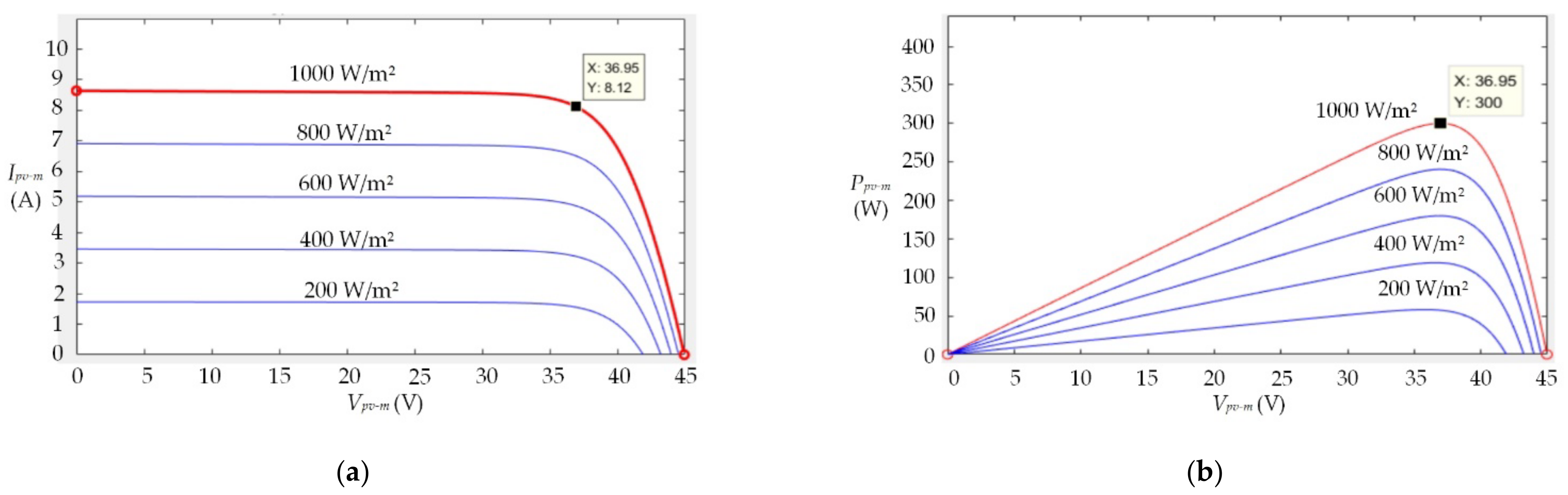
Figure 1 displays the single PV-M that was used during the experiment. This single PV-M used a Chroma PV-M simulator (model number 62020H-150S). At irradiance level (G) 1000 W/m² and temperature (T) 25 °C, PV-M V_oc = 44.95 V, I_sc = 8.64 A, V_MPP = 36.95 V, I_MPP = 8.12 A, and P_MPP = 300 W (as shown in

Table 2. The parameters of the photovoltaic module.

Parameter	Value
PV-M open circuit voltage (Voc)	44.95 V
PV-M short circuit current (Isc)	8.64 A
PV-M maximum power point voltage (VMPP)	36.95 V
PV-M maximum power point current (IMPP)	8.12 A
PV-M maximum power (PMPP)	300 W
PV-M temperature coefficient of Voc	−0.36901 V/°C
PV-M temperature coefficient of Isc	0.06099 A/°C

). Figure 1a illustrates the PV-M I_pv-m–V_pv-m characteristic curve graph at temperature 25 °C and the irradiance levels 200 W/m², 400 W/m², 600 W/m², 800 W/m², and 1000 W/m², respectively. Figure 1b shows the PV-M P_pv-m–V_pv-m characteristic curve graph at a temperature of 25 °C and the irradiance levels 200 W/m², 400 W/m², 600 W/m², 800 W/m², and 1000 W/m², respectively.

The relationship among PV-M P_pv-m, V_pv-m, and R_pv-m is as follows:

$$R_{pv-m}=\frac{V_{pv-m}^2}{P_{pv-m}}$$

(1)

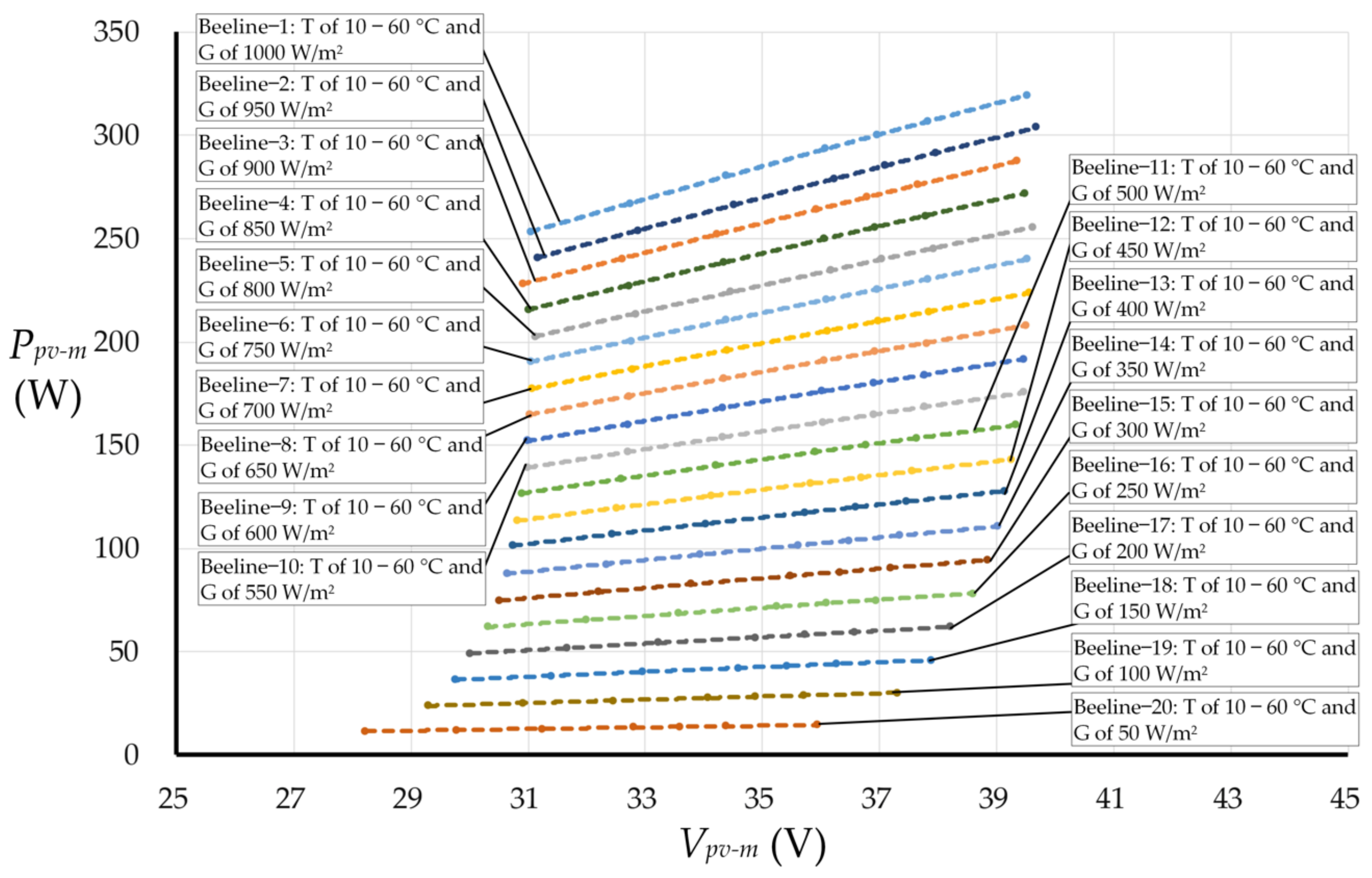
First, this study analyzed the PV-M I_pv-m–V_pv-m characteristic curves as in Figure 1a and PV-M P_pv-m–V_pv-m characteristic curves as in Figure 1b and used Microsoft Excel to draw the relationship among V_pv-m, P_pv-m, temperature, and irradiance level beelines (as shown in Figure 2). Figure 2 demonstrates that twenty beelines were drawn to show the relationship among V_pv-m, P_pv-m, temperature, and irradiance level, where the temperatures (T) are from 10 °C to 60 °C, and the irradiance levels (G) are 50 W/m², 100 W/m², 150 W/m², 200 W/m², 250 W/m², 300 W/m², 350 W/m², 400 W/m², 450 W/m², 500 W/m², 550 W/m², 600 W/m², 650 W/m², 700 W/m², 750 W/m², 800 W/m², 850 W/m², 900 W/m², 950 W/m², and 1000 W/m², respectively. The Beeline-1 to Beeline-20 were depicted PV-M output power (P_pv-m) that the PV-M output maximum power (P_MPP).The mathematical model for the twenty beelines could be approximated as the following quadratic equation:

$$P_{pv-m}=x_1\cdot V_{pv-m}^2+y_1\cdot V_{pv-m}+z_1$$

(2)

where x₁, y₁, and z₁ are parameters. Equation (2) shows the relationship between the parameters of x₁, y₁, and z₁, irradiance level, and temperature, as shown in

Table 3. Relationship between the x₁, y₁, and z₁ parameters, irradiance level, and temperature.

Irradiance Level (W/m2)	Temperature (°C)	Parameter
		x1	y1	z1
1000	10−60	−0.0432	10.85	−41.88
950	10−60	−0.0408	10.275	−39.81
900	10−60	−0.0392	9.81	−37.69
850	10−60	−0.0369	9.25	−35.64
800	10−60	−0.0344	8.66	−33.50
750	10−60	−0.0324	8.15	−31.47
700	10−60	−0.0302	7.59	−29.32
650	10−60	−0.0281	7.06	−27.25
600	10−60	−0.0260	6.52	−25.13
550	10−60	−0.0238	5.97	−23.01
500	10−60	−0.0218	5.45	−20.94
450	10−60	−0.0196	4.89	−18.76
400	10−60	−0.0178	4.40	−16.98
350	10−60	−0.0155	3.82	−14.70
300	10−60	−0.0133	3.27	−12.54
250	10−60	−0.0112	2.73	−10.38
200	10−60	−0.0091	2.18	−8.24
150	10−60	−0.0068	1.63	−6.11
100	10−60	−0.0046	1.09	−3.99
50	10−60	−0.0024	0.55	−1.93

.

V_pv-m^G is determined via Equation (3), as follows:

$$V_{pv-m}^{\mathrm{G}}=\frac{-y_1+\sqrt{y_1^2-4\cdot x_1\cdot \left(z_1-P_{pv-m}\right)}}{2\cdot x_1}$$

(3)

Different irradiance levels correspond to different parameters of x₁, y₁, and z₁. First, Equation (3) and Table 3 were used to calculate 20 sets of V_pv-m^G of the irradiance levels 50 W/m², 100 W/m², 150 W/m², 200 W/m², 250 W/m², 300 W/m², 350 W/m², 400 W/m², 450 W/m², 500 W/m², 550 W/m², 600 W/m², 650 W/m², 700 W/m², 750 W/m², 800 W/m², 850 W/m², 900 W/m², 950 W/m², and 1000 W/m². Second, the actual V_pv-m were compared with the 20 sets of V_pv-m^G. Finally, the algorithm chose the closest set of V_pv-m^G to calculate the corresponding irradiance level (as shown in Table 3).

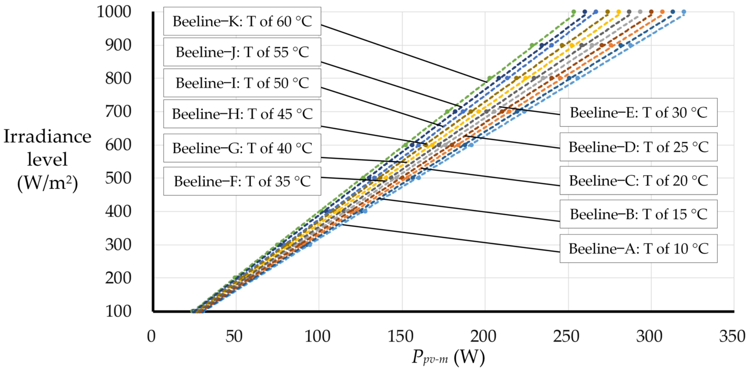
As shown in Figure 1a, the PV-M P_pv-m–V_pv-m characteristic curves were analyzed, and as shown in Figure 1b, the PV-M I_pv-m–V_pv-m characteristic curves were analyzed. Then, Microsoft Excel was used to draw the relationship among irradiance level, P_pv-m, and the temperature (T) beelines (as shown in Figure 3). Figure 3 demonstrates the following eleven beelines that were drawn through the relationship among irradiance level, P_pv-m, and temperature (T): Beeline-A to Beeline-K present the characteristics at an irradiance level (G) from 100 W/m² to 1000 W/m² and the temperatures 10, 15, 20, 25, 30, 35, 40, 45, 50, 55, and 60 °C, respectively. Beeline-A to Beeline-K were depicted PV-M output power (P_pv-m) that the PV-M output maximum power (P_MPP). In addition, to express the parameter w equation, the mathematical model for the eleven beelines (as shown in Figure 3) could be approximated using the following equation:

$$w={\mathrm{G}}^{1.0256}\cdot P_{pv-m}^{-1}$$

(4)

where the parameter w is the compensation parameter that corresponds to the relationship of temperature. Figure 3 and Equation (4) show the relationship between parameter w and temperature, as shown in

Table 4. Relationship between the parameter w and temperature.

Temperature	Parameter w
10 °C	3.5751
15 °C	3.6474
20 °C	3.7227
25 °C	3.8018
30 °C	3.8842
35 °C	3.9715
40 °C	4.0628
45 °C	4.1599
50 °C	4.2618
55 °C	4.3693
60 °C	4.4826

.

Table 4 displays the relationship between parameter w and temperature. According to Equation (4) and Table 4, it was found that parameter w could be obtained by the relationship between irradiance level and P_pv-m.

Under UIC, the proposed global-MPPT algorithm calculates the parameter w of 3.5751 to 4.4826 from a temperature of 10 °C to 60 °C (as shown in Table 4). If the parameter w was lower than 3.5751 or higher than 4.4826, the PV-M was under a PSC.

In this research, the PV-M was connected with the boost converter, and the boost converter was connected to the load. Under ideal conditions, P_pv-m = P_o, and the relationship among PV-M impedance (R_pv-m), load (R_o), and duty cycle (D) is expressed as follows:

$$R_o^{}=R_{pv-m}^{}\cdot \frac{1}{{(1-D)}^2}$$

(5)

PV-M impedance (R_pv-m), load (R_o), and duty cycle (D) can be obtained through Equation (6):

$$\mathrm{D}=1-\sqrt{R_{pv-m}^{}\cdot R_o^{-1}}$$

(6)

Applying Equations (1) and (4) in Equation (6) yields the following equation for the relationship among PV-M output voltage (V_pv-m), parameter w, duty cycle (D), irradiance level (G), and load (R_o):

$$\mathrm{D}=1-\sqrt{\frac{V_{pv-m}^2\cdot w}{R_o\cdot {\mathrm{G}}^{1.0256}}}$$

(7)

Equation (7) considers load (R_o), actual irradiance level (G), PV-M output voltage (V_pv-m), and parameter w, where the parameter w is the compensation parameter that corresponds to the relationship of temperature (as shown in Table 4). Thereby, D is the duty cycle of the global-MPPT.

The duty cycle can also be calculated by Equation (6). However, in this study the proposed global-MPPT algorithm analyzed the PV-M I_pv-m–V_pv-m characteristic curves and PV-M P_pv-m–V_pv-m characteristic curves that obtain the relationship between irradiance level and temperature, then judges the duty cycle of the MPP from irradiance level (G), parameter w, load (R_o), and PV-M output voltage (V_pv-m) (as in Equation (7)). The proposed global-MPPT algorithm has the following advantages: first, the MPPT follows the actual irradiance level and temperature in accordance with the laws of nature. Second, Equations (1)–(7) and Table 2, Table 3 and Table 4 all have the compensating parameters for MPPT optimization. Finally, Equation (7) has many compensating parameters and is calculated carefully. Therefore, the proposed global-MPPT algorithm can provide a soft duty cycle of the MPPT to the power converter to reduce switching stress and enhance system performance.

In this study, according to Figure 1, Figure 2 and Figure 3, Equations (1)–(7) and Table 2, Table 3 and Table 4 are the theoretical basis, where several parameters are compensated to ensure the reliability and accuracy of the MPPT. The proposed global-MPPT algorithm could immediately capture the MPP under a UIC and PSC. The proposed method has high performance that improves the shortcomings of the P&O algorithm: first, the algorithm has no disturbance characteristics; second, the actuating point would not be disturbed near the MPP; third, the algorithm can catch the MPP under a PSC; finally, this algorithm’s convergence speed is high. In conclusion, this proposed global-MPPT algorithm is not a continuous iterative estimation, which reduces the MPPT tracking time. This algorithm also decreases the operating complexity of the microcontroller unit (MCU). Therefore, the proposed global-MPPT algorithm is better than the PSO algorithm.

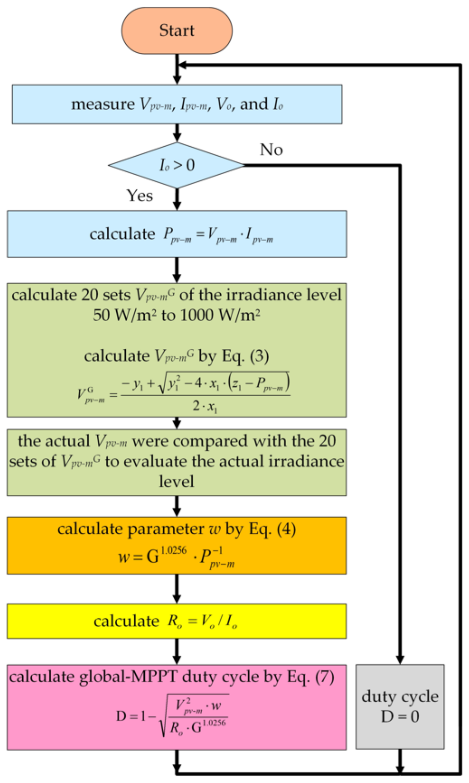
Figure 4 displays the proposed global-MPPT algorithm flowchart. V_pv-m is the PV-M output voltage; I_pv-m is the PV-M output current; V_o represents the boost converter output voltage; I_o represents the boost converter output current; x₁, y₁, and z₁ are the parameters of Equation (3); parameter w is from Equation (4); and D is the global-MPPT duty cycle of Equation (7). First, the proposed global-MPPT algorithm was used to measure V_pv-m, I_pv-m, V_o, and I_o and calculate P_pv-m. Second, Equation (3) calculated 20 sets of V_pv-m^G of the irradiance levels 50 W/m², 100 W/m², 150 W/m², 200 W/m², 250 W/m², 300 W/m², 350 W/m², 400 W/m², 450 W/m², 500 W/m², 550 W/m², 600 W/m², 650 W/m², 700 W/m², 750 W/m², 800 W/m², 850 W/m², 900 W/m², 950 W/m², and 1000 W/m², and the actual V_pv-m were compared with the 20 sets of V_pv-m^G to evaluate the actual irradiance level (G). Third, the proposed method determined parameter w using Equation (4). Fourth, the proposed global-MPPT algorithm calculated R_o. Lastly, the global-MPPT duty cycle (D) was calculated by Equation (7), which includes the parameters irradiance level (G), load (R_o), PV-M output voltage (V_pv-m), and parameter w. In addition, if I_o was less than zero, the duty cycle would = 0.

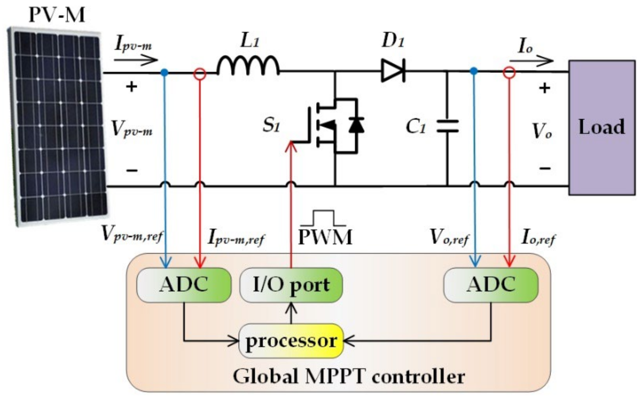
Figure 5 shows the diagram of the boost converter with the proposed global-MPPT algorithm, where the PV-M is connected to the boost converter for power electronics [38,39] and the proposed global-MPPT algorithm is embedded. The PV-M was a Chroma PV-M simulator (model number: 62020H-150S). When G = 1000 W/m² and T = 25 °C, V_oc = 44.95 V, I_sc = 8.64 A, V_MPP = 36.95 V, I_MPP = 8.12 A, and P_MPP = 300 W (as shown in Table 2). The boost converter elements include inductor L₁ (L₁ of 0.6 mH), capacitor C₁ (C₁ of 470 μF), diode D₁, and power MOSFET (S₁). In this circuit, the V_pv-m, I_pv-m V_o, and I_o signals were sent to the MPPT controller’s MCU. The global-MPPT controller (Microchip, model number: 18F452) provides the PWM signal (frequency = 45 kHz) to drive the boost converter’s power MOSFET (S₁) so that the proposed system can search for the MPP and then catch the MPP.

4. Experimental Results

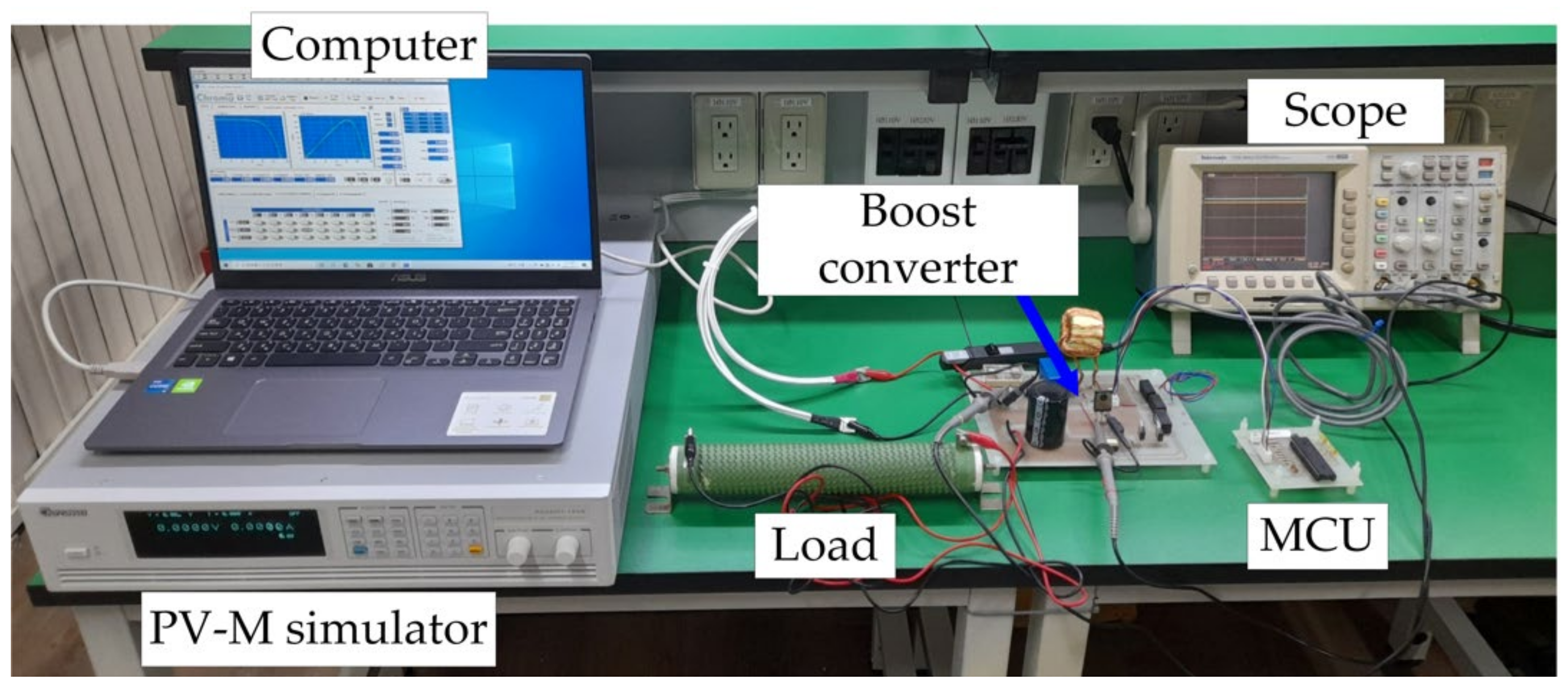
Figure 6 presents the experimental PV-M simulator and the proposed global-MPPT algorithm prototype test setup. The PV-M simulator (Chroma, model number: 62020H-150S) was set at the following specifications: V_oc = 44.95 V, I_sc = 8.64 A, V_MPP = 36.95 V, I_MPP = 8.12 A, and P_MPP = 300 W under the irradiance level (G) = 1000 W/m² and temperature (T) = 25 °C. In the test, the PV-M simulator was connected to the input of the boost converter, and the load was connected to the output of the boost converter. The MCU implemented the global-MPPT algorithm and provided the PWM signal to drive the boost converter and reach the MPP.

The MPPT efficiencies of the proposed global-MPPT algorithm, the PSO algorithm, and the P&O algorithm were tested experimentally under a UIC in which the irradiance level (G) is 800 W/m² and 300 W/m², respectively. As shown in Figure 7, Figure 8, Figure 9 and Figure 10 and

Table 5. A comparison of three algorithms’ MPPT efficiency under UIC.

Algorithm	G = 800 W/m2 and T = 25 °C			G = 300 W/m2 and T = 50 °C
	PMPP (W)	Ppv-m (W)	Efficiency (%)	PMPP (W)	Ppv-m (W)	Efficiency (%)
Proposed	240	239.8	99.9	80	79.8	99.8
PSO	240	239.8	99.9	80	79.7	99.6
P&O	240	239.5	99.8	80	78	97.5

, the results show that the efficiency of the proposed global-MPPT algorithm’s MPPT was better than those of the PSO and P&O algorithms.

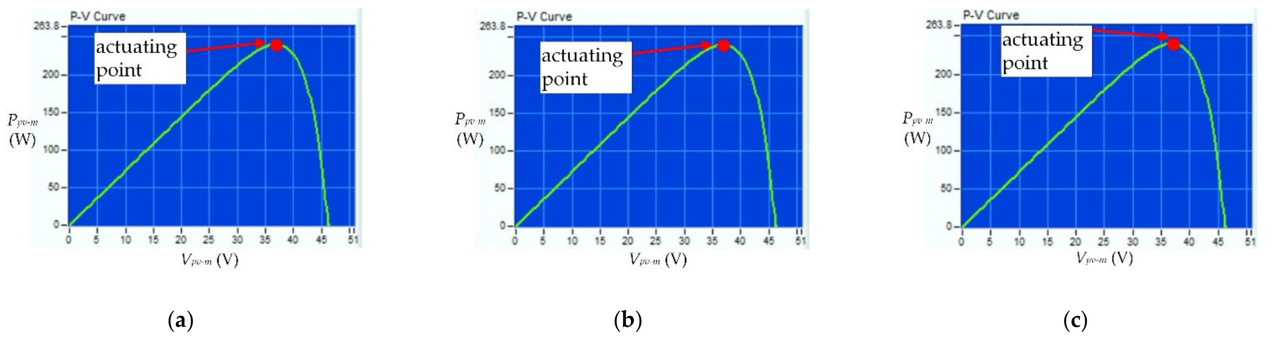
Figure 7 displays the test results for the proposed global-MPPT algorithm, PSO algorithm, and P&O algorithm under a UIC in which irradiance level (G) = 800 W/m², and temperature (T) = 25 °C. Figure 7a illustrates the proposed global-MPPT algorithm experiment results. First, the proposed global-MPPT algorithm sensed V_pv-m = 37.2 V, P_pv-m = 225 W, and R_o = 6 Ω. 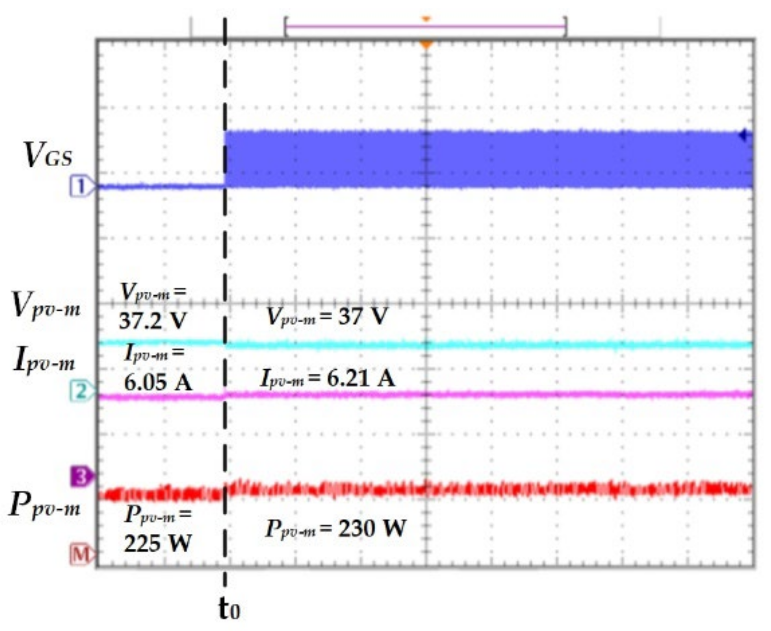Second, the proposed global-MPPT algorithm calculated V_pv-m^G = 37 V by Equation (3), and the actual V_pv-m was compared with the V_pv-m^G to evaluate the actual irradiance level (G) = 800 W/m² (as shown in Table 3), then calculated parameter w = 3.8 by Equation (4), and the proposed global-MPPT algorithm estimated that the PV-M was under a UIC. Finally, it calculated the global-MPPT D = 0.5 by Equation (7). When time = t₀ (as shown in Figure 8), the proposed global-MPPT algorithm started, then the proposed global-MPPT algorithm reached the MPP, where the measured results are V_MPP = 37 V, I_MPP = 6.21 A, and P_MPP = 230 W (as in Figure 7a and Figure 8). The proposed global-MPPT algorithm could be accurately and stably operated at the MPP with a system efficiency of 99.9%.

Figure 7b displays the PSO algorithm test results. This algorithm performed iterative calculations and could operate at the MPP with an MPPT efficiency of 99.9%. Figure 7c displays the P&O algorithm test results. The algorithm detected the slope of the PV-M output power and PV-M output voltage and then operated the MPP. The algorithm’s MPPT efficiency was 99.8% (as shown in Table 5).

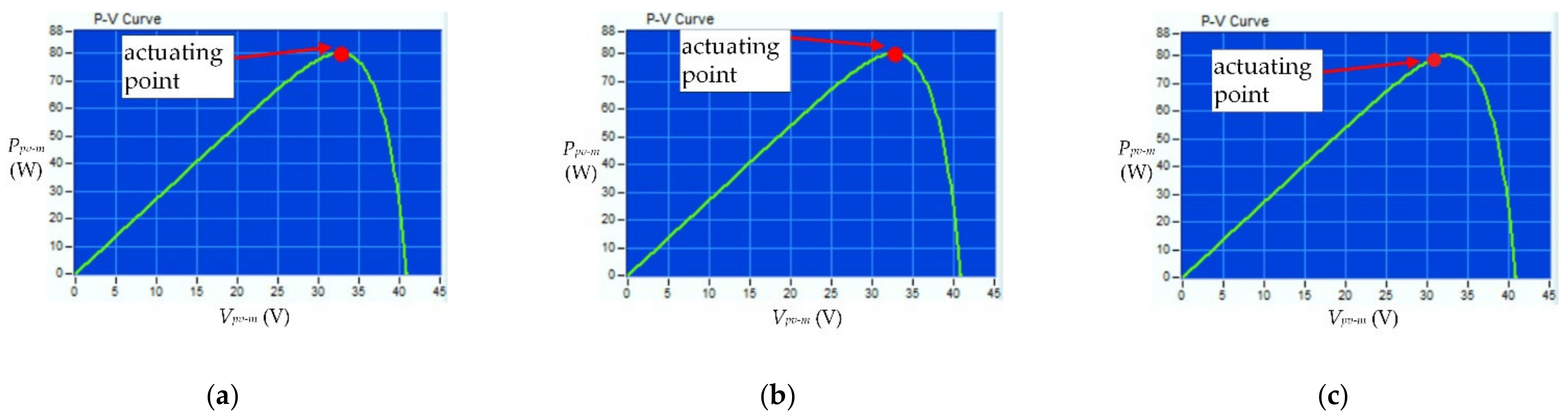
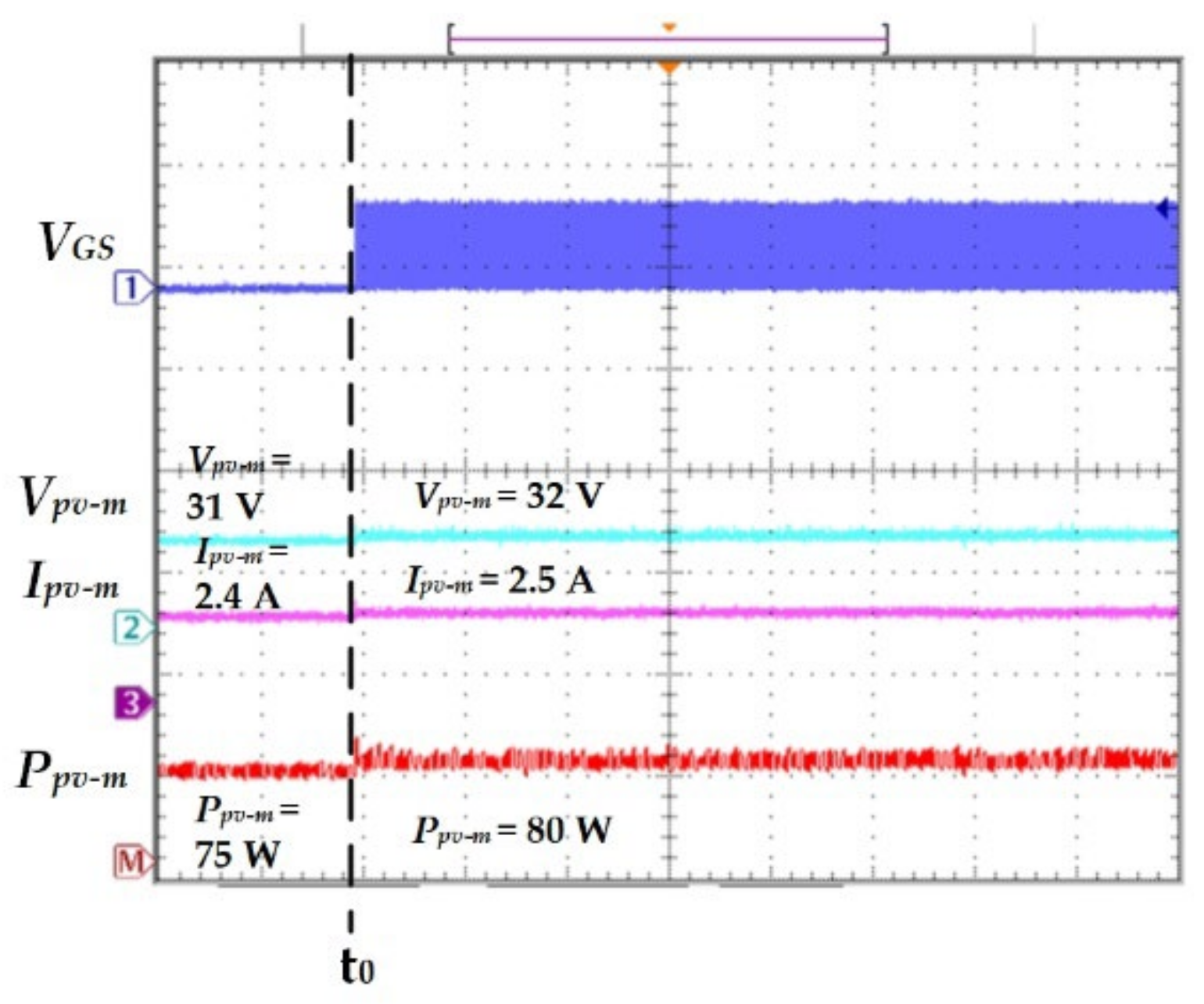
Figure 9 illustrates the test results for the proposed global-MPPT algorithm, the PSO algorithm, and the P&O algorithm under a UIC in which irradiance level (G) = 300 W/m² and temperature (T) = 50 °C. Figure 9a illustrates the proposed global-MPPT algorithm test results. First, the proposed global-MPPT algorithm measured V_pv-m = 31 V, P_pv-m = 75 W, and R_o = 13 Ω. Second, the proposed global-MPPT algorithm calculated V_pv-m^G = 32 V using Equation (3), and the actual V_pv-m was compared with the V_pv-m^G to evaluate the actual irradiance level (G) = 300 W/m² (as shown in Table 3), then calculated parameter w = 4.3 using Equation (4), and the proposed global-MPPT algorithm estimated that the PV-M was under a UIC. Finally, it calculated global-MPPT D = 0.05 using Equation (7). When time = t₀ (as shown in Figure 10), the proposed global-MPPT algorithm started, then the proposed global-MPPT algorithm reached the MPP, where the measured results were V_MPP = 32 V, I_MPP = 2.5 A, and P_MPP = 80 W (as in Figure 9a and Figure 10). The proposed global-MPPT algorithm could be accurately and stably operated at the MPP, with a system efficiency of 99.8%.

Figure 9b displays the PSO algorithm test results. This algorithm was an iterative calculation, and it could operate at the MPP with an MPPT efficiency of 99.6%. Figure 9c displays the P&O algorithm test results. The algorithm detected the slope of the PV-M output power and the PV-M output voltage and then operated at the MPP. As the algorithm actuating point vibrated, the MPPT efficiency was 97.5% (as shown in Table 5).

Table 5 shows the comparison among the three algorithms’ MPPT efficiencies under a UIC. The proposed global-MPPT algorithm had MPPT efficiency of 99.9% and 99.8% under 800 W/m² and 300 W/m², respectively. In addition, the proposed global-MPPT algorithm’s efficiency was higher than those of the PSO and P&O algorithms. Therefore, this experiment proved that the proposed global-MPPT algorithm had higher efficiency and was suitable for different irradiance levels and temperatures.

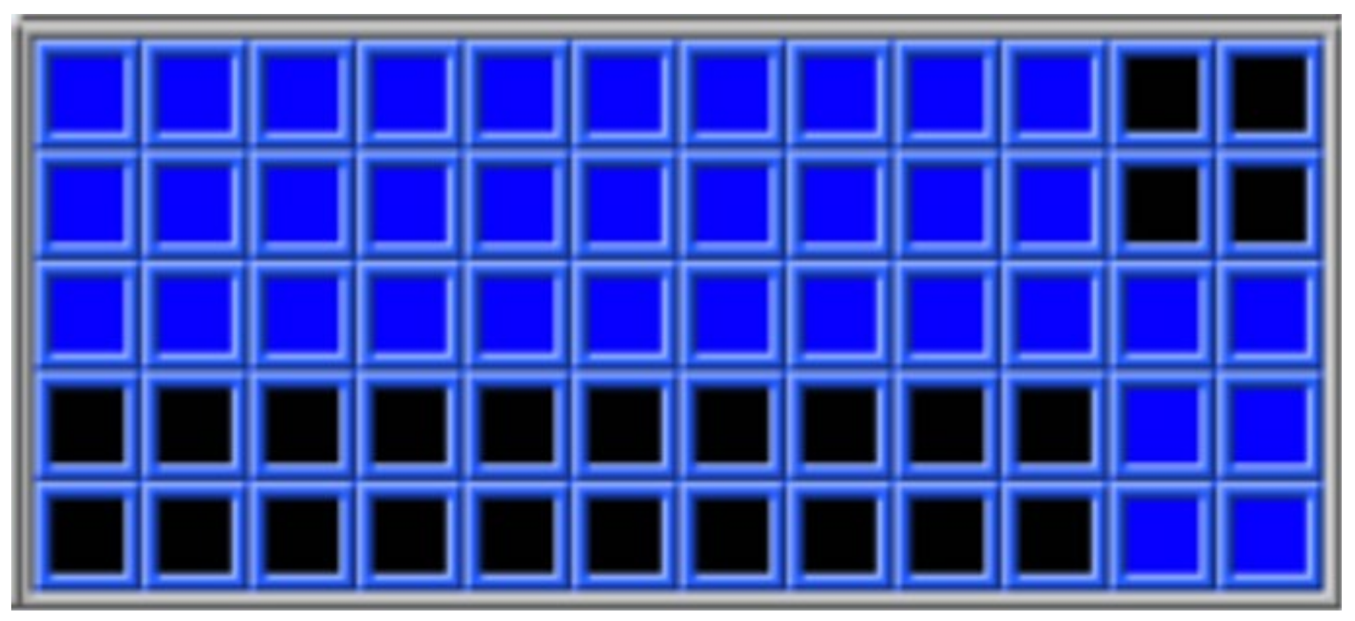
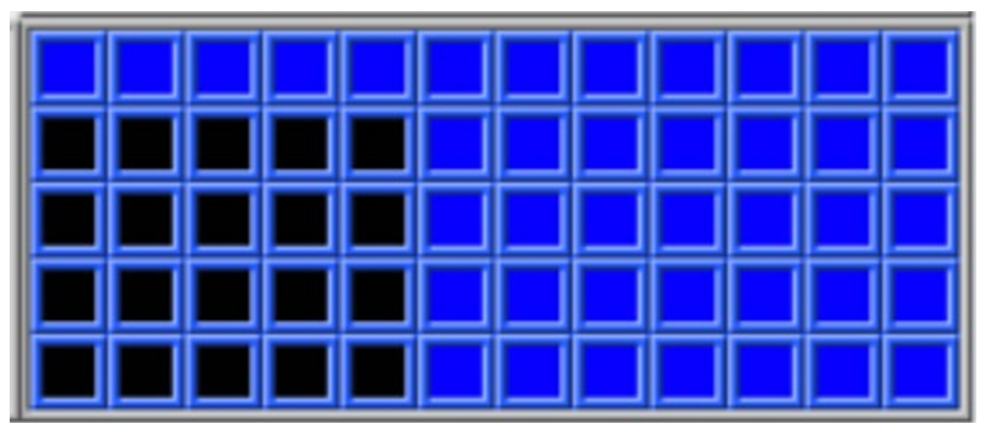
The MPPT efficiencies of the proposed global-MPPT algorithm, the PSO algorithm, and the P&O algorithm were tested experimentally under a PSC. Figure 11 displays the diagram of the PV-M’s solar cell array for shadow simulation through single PV-M simulator software in this study. The structure of the PV-M’s solar cell array was 12 × 5. In this test, under a PSC in which irradiance level (G) = 900 W/m², temperature (T) = 25 °C, twenty-four solar cells were shaded in the PV-M (represented by the black square shown in Figure 11). Then, the PV-M’s characteristics were measured, where V_MPP = 29.9 V, I_MPP = 4.23 A, and P_MPP = 126.6 W. These test results show that the MPPT efficiency of the proposed global-MPPT algorithm was better than those of the PSO and P&O algorithms, as shown in Figure 12 and Figure 13, and

Table 6. A comparison among three algorithms’ MPPT efficiency under PSC.

Algorithm	G = 900 W/m2 and T = 25 °C			G = 600 W/m2 and T = 40 °C
	PMPP (W)	Ppv-m (W)	Efficiency (%)	PMPP (W)	Ppv-m (W)	Efficiency (%)
Proposed	126.6	126.2	99.7	100	99.5	99.5
PSO	126.6	117.5	92.8	100	95.1	95.1
P&O	126.6	49.1	38.8	100	28.5	28.5

.

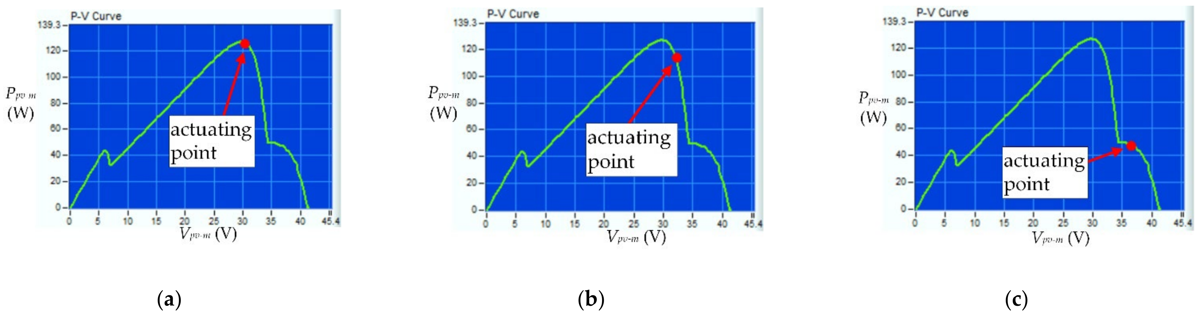
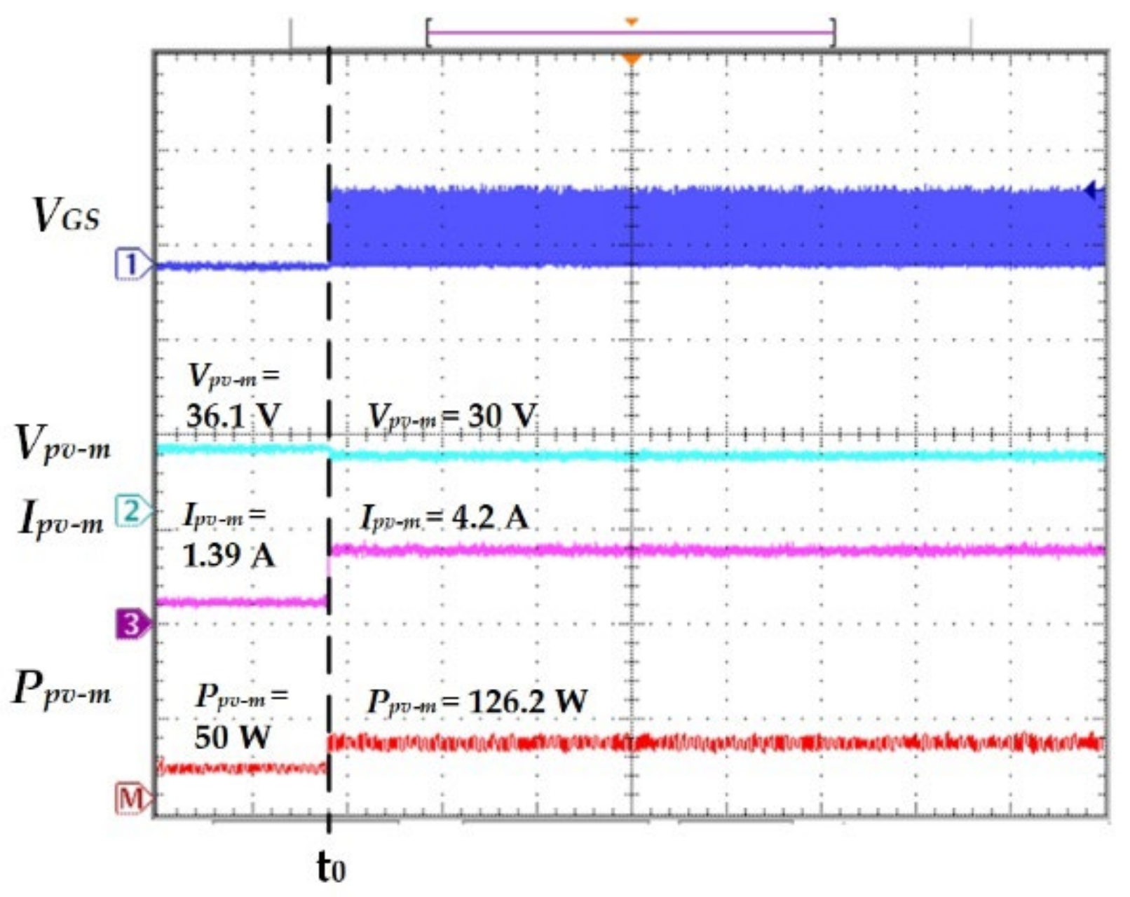
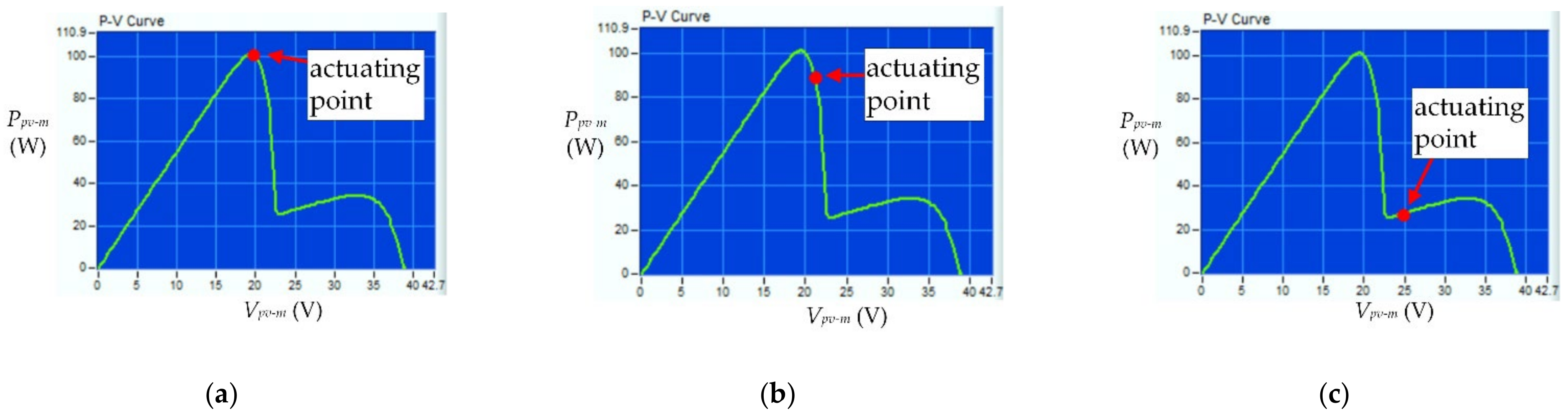
Figure 12 illustrates test results for the proposed global-MPPT algorithm, PSO algorithm, and P&O algorithm under a PSC in which irradiance level (G) = 900 W/m² and temperature (T) = 25 °C. Figure 12a illustrates the test results for the proposed global-MPPT algorithm. First, the proposed global-MPPT algorithm measured V_pv-m = 36.1 V, P_pv-m = 50 W, and R_o = 28 Ω. Second, the proposed global-MPPT algorithm calculated V_pv-m^G = 36.7 V using Equation (3), and the actual V_pv-m was compared with the V_pv-m^G to evaluate the actual irradiance level (G) = 900 W/m² (as shown in Table 3), then calculated parameter w = 21.2 using Equation (4), and the proposed global-MPPT algorithm estimated that the PV-M was under a PSC. Finally, it calculated the global-MPPT D = 0.05 using Equation (7). When time = t₀ (as shown in Figure 13), the proposed global-MPPT algorithm starts, the proposed global-MPPT algorithm reached the global MPP, and then measured results that V_MPP = 30 V, I_MPP = 4.2 A, and P_MPP = 126.2 W (as in Figure 12a and Figure 13). The proposed global-MPPT algorithm considered the irradiance level and load, etc. Therefore, under a PSC, the proposed global-MPPT algorithm could be accurately and stably operated at the global MPP, with a system efficiency of 99.7%.

Figure 12b displays the PSO algorithm test results. This algorithm was an iterative calculation and searched for the global MPP. However, the algorithm’s execution time was longer than that for the proposed global-MPPT algorithm and it could not capture the global MPP in time, therefore the MPPT efficiency was 92.8%. Figure 12c displays the P&O algorithm test results. The algorithm detected the slope of the PV-M output power and the PV-M output voltage, and then searched for the global MPP. However, the algorithm became trapped in the local MPP. Therefore, the MPPT efficiency was 38.8% (as shown in Table 6).

Figure 14 shows that the combination of the PV-M’s solar cell array was 12 × 5. In this test, under a PSC in which irradiance level (G) = 600 W/m², temperature (T) = 40 °C, and twenty solar cells were shaded in the PV-M (represented by the black squares shown in Figure 14), PV-M V_MPP = 19.6 V, I_MPP = 5.1 A, and P_MPP = 100 W. The test results show that the MPPT efficiency of the proposed global-MPPT algorithm was better than those of the PSO and P&O algorithms, as shown in Figure 15 and Figure 16, and Table 6.

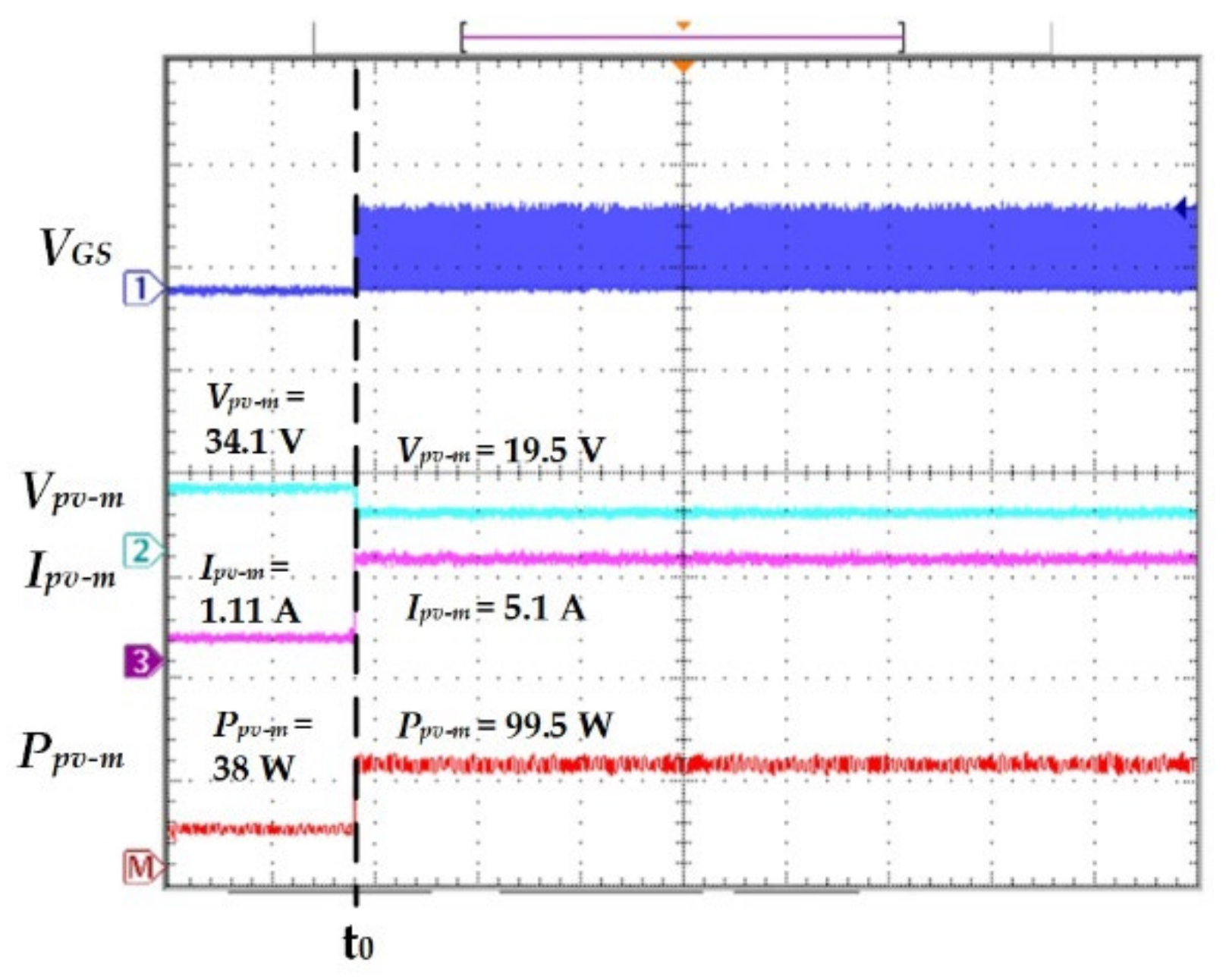
Figure 15 shows the test results for the proposed global-MPPT algorithm, the PSO algorithm, and the P&O algorithm, under a PSC in which irradiance level (G) = 600 W/m² and temperature (T) = 40 °C. Figure 15a illustrates the proposed global-MPPT algorithm test results. First, the proposed global-MPPT algorithm sensed V_pv-m = 34.1 V, P_pv-m = 38 W, and R_o = 30 Ω. Second, the proposed global-MPPT algorithm calculated V_pv-m^G = 34.3 V using Equation (3), and the actual V_pv-m was compared with the V_pv-m^G to evaluate the actual irradiance level (G) = 600 W/m² (as shown in Table 3), then calculated parameter w = 18.1 using Equation (4), and the proposed global-MPPT algorithm estimated that the PV-M was under a PSC. Finally, it calculated the global-MPPT D = 0.03 using Equation (7). When time = t₀ (as shown in Figure 16) the proposed global-MPPT algorithm starts up, then the proposed global-MPPT algorithm reached the global MPP, and measured results that V_MPP = 19.5 V, I_MPP = 5.1 A, and P_MPP = 99.5 W (as in Figure 15a and Figure 16). The proposed global-MPPT algorithm considered the irradiance level and the load, etc. Therefore, the proposed global-MPPT algorithm under a PSC could be accurately and stably operated at the global MPP (as shown in Figure 12a), with a system efficiency of 99.5%.

Figure 15b displays the PSO algorithm test results. This algorithm was an iterative calculation and searched for the global MPP. However, the algorithm’s execution time was longer than that of the proposed global-MPPT algorithm, and it could not capture the global MPP in time (as shown in Figure 12b). Therefore, the MPPT efficiency was 95.1%. Figure 15c displays the P&O algorithm test results. The algorithm detected the slope of the PV-M output power and the PV-M output voltage, and then searched for the global MPP. However, the algorithm became trapped in the local peak power point (as shown in Figure 12c). Therefore, the MPPT efficiency was 28.5% (as shown in Table 6).

Table 6 shows a comparison among the three algorithms’ MPPT efficiency under a PSC. The proposed global-MPPT algorithm’s MPPT efficiency was 99.7% and 99.5% under 900 W/m² and 600 W/m², respectively. In addition, the proposed global-MPPT algorithm’s efficiency was better than those of the PSO and P&O algorithms. Therefore, this experiment proved that the proposed global-MPPT algorithm had high efficiency and was suitable for a PSC.

5. Conclusions

In this study, the proposed global-MPPT algorithm was proposed to analyze the irradiance level, the output voltage, and the output power of the PV-M. In the proposed algorithm, the important parameter w is determined by the PV-M output power and irradiance level, which is also the compensation parameter that corresponds to the relationship of temperature. The proposed global-MPPT algorithm was developed to predict the best duty cycle for the global-MPPT based on the irradiance level, parameter w, PV-M output voltage, and load so that the PV-M can achieve the MPP quickly and accurately. The test results verified that under a UIC, the proposed global-MPPT algorithm’s MPPT efficiency was 99.9% and 99.8% under 800 W/m² and 300 W/m², respectively. In addition, under a PSC, the proposed global-MPPT algorithm’s MPPT efficiency was 99.7% and 99.5% under 900 W/m² and 600 W/m², respectively. In summary, under a UIC and PSC, the proposed global-MPPT algorithm’s MPPT performed better than the PSO and P&O algorithms.

The proposed global-MPPT algorithm considered the change in the irradiance level, parameter w, PV-M output voltage, and load. Therefore, under a UIC and PSC, the proposed global-MPPT algorithm could quickly and accurately capture the MPP. The proposed system of this study did not require a complex power electronic circuit architecture and complex calculation. Further, it could accurately reach the MPP and greatly reduce the design cost.

In future work, the proposed global-MPPT algorithm uses two voltage sensors and two current sensors that increase manufacturing costs. In the future, the research can focus on reducing sensors with new MPPT algorithms to reach lower costs and complexity. The proposed global-MPPT algorithm can be applied to rooftop solar power systems, which are often shaded. The proposed global-MPPT algorithm could improve the power generation efficiency of these solar power systems. In addition, future studies can develop a novel power electronic converter that solves the shadowing problem. Combining this novel power electronic converter with the proposed global-MPPT algorithm could take PSC research on PV-Ms to the next level.