
Novel Fuzzy Measurement Alternatives and Ranking according to the Compromise Solution-Based Green Machining Optimization


1
Department of Mechanical Engineering, Sri Sairam Institute of Technology, Chennai 60044, India
2
School of Mechanical Engineering, Vellore Institute of Technology, Chennai 600127, India
3
Department of Machining, Assembly and Engineering Metrology, Faculty of Mechanical Engineering, VSB-Technical University of Ostrava, 70800 Ostrava, Czech Republic
4
Department of Mechanical Engineering, Vel Tech Rangarajan Dr. Sagunthala R&D Institute of Science and Technology, Avadi 600062, India
*
Authors to whom correspondence should be addressed.
Processes 2022, 10(12), 2645; https://doi.org/10.3390/pr10122645
Submission received: 28 July 2022
/
Revised: 20 November 2022
/
Accepted: 7 December 2022
/
Published: 8 December 2022
Abstract
:Due to the increase in the impact of different manufacturing processes on the environment, green manufacturing processes are the prime focus of many current pieces of research. In the current article, a green machining process for stainless steel and SS304 and AISI1045 steel has been optimized using newly developed Fuzzy Measurement Alternatives and Ranking according to the COmpromise Solution (F-MARCOS) method in the form of two case studies. In the first case study, nose radius, cutting speed, depth of cut, and feed rate are selected as the process parameters whereas surface roughness, consumption of electrical energy, and power factor are the outputs. In the second case study width of cut, depth of cut, feed rate, and cutting speed were the process parameters and material removal rate (MRR), active energy consumption (ACE), and surface roughness (Ra) are the response variables. The MARCOS method ranks the alternatives based on the ideal and anti-ideal solutions for the different criteria. The inclusion of fuzzy logic adds worth to the model by using a linguistic scale to make the method more practical and flexible. Based on the detailed analysis, it ranked the best alternative in case study one which results in a power factor of 0.862, 26.68 kJ of electrical energy consumption, and surface roughness of 0.36 . In the second case study, the best alternative selected by this method gave an MRR of 2400 and Ra of 2.29 and utilizes 53.988 kJ ACE.
1. Introduction
Green manufacturing refers to the manufacturing of goods with lesser environmental impacts and higher safety for workers [1]. During machining operations to improve the quality of the product and the life of the tool, different lubricants are being used which causes the generation of harmful gases and affects the health of workers as well as the environment. To overcome this issue, minimum quantity lubrication and dry machining processes have been applied [2,3,4,5,6], where much less or no lubricant is used which is eco-friendly as well as cost-effective. As the awareness of environmental issues is increasing, dry machining is becoming more crucial.
In the case of the milling process, removal of workpiece material takes place by pressing the rotating cutter towards the workpiece material in the presence of lubricant (lubricated) or in the absence of lubricant (dry). Environmental issues related to the use of lubricant have been discussed already, so in this article, the work of the dry milling process is analyzed. Any process is affected by operating conditions and different parameters. A lot of research has been done to study the effect of these parameters on the machining process by considering various outputs such as surface roughness, tool wear, cutting forces, etc. [7,8,9,10]. Therefore, the selection of these parameters plays an important role in the machining process. There are various techniques which have been used by different researchers to obtain the best combinations of these machining parameters such as Genetic Algorithm [11], Taguchi optimization [12], various kinds of multicriteria decision methods (MCDMs) such as the technique for order of preference by similarity to ideal solution (TOPSIS) [13], multi-objective optimization based on ratio analysis (MOORA) [14], gray relational analysis (GRA) [15], particle swarm optimization (PSO) [16], etc. With the development of these mathematical techniques, these MCDMs are also being used along with fuzzy logic to get more precise parametric combinations.
Stankovic et al. [17] used Fuzzy MARCOS for the road traffic risk analysis, Taş et al. [18] used this for supply chain management, Ali [19] applied it in solid waste management, Bakir and Atalik [20] used this method for evaluating the e-service quality in the airline industry, Kovač et al. [21] studied it for assessment of drone-based city logistics concepts, etc., and reached a conclusion that this method is significantly stable and reliable in the dynamic situations as well as for larger datasets.
Generally, in conventional optimization, either equal importance to each response is given or they are studied individually as single objective optimization. The different optimal combinations for the desired output are then computed. However, in the actual situation consumers or users have different types of expectations of the final product, some of which may be contradictory. Therefore, this work is motivated by the same problem and tries to solve this issue by amalgamating the concept of MCDMs and fuzzy theory. Specifically, the article makes the following contributions—
- A newly developed MCDM technique Measurement Alternatives and Ranking according to the COmpromise Solution (MARCOS) in conjunction with fuzzy theory is used to obtain the optimum combination of green milling parameters for machining of SS 304 and AISI 1045 steel. To the best of the authors’ knowledge, Fuzzy-MARCOS has so far not been used for machining process optimization.
- A linguistic scale is developed using Triangular Fuzzy Numbers (TFNs) to consider different expectations of the product by different users.
- The proposed Fuzzy MARCOS utilizes fuzzy ideal and anti-ideal solutions for referencing, it also provides a more precise utility degree, and a large set of alternatives and criteria is considered for the analysis as well as makes the problem more realistic by defining the linguistic scale based on TFNs.
- This article considers cutting speed (), depth of cut (), feed rate (), and nose radius () as the input variables to optimize the ratio of active to apparent power consumption (PF), active cutting energy (ACE), and surface roughness (Ra) as the response variables.
2. Methodology
A machining process requires a large amount of energy to remove material from the workpiece to obtain the desired shape. The amount of energy required depends upon the combination of different machining parameters such as cutting speed, feed depth of cut and method of lubrication etc. To rate the quality of the machining, we consider various response variables such as surface roughness, cutting force, tool wear, vibration, etc. When it comes to green machining, the manufacturer must consider manufacturing aspects (e.g., rate of removal of material, surface finish, wear, tear of tool, etc.) as well as environmental aspects (e.g., power consumed, scrap produced, temperature, etc.). In the current work, dry two cases for dry milling are considered for decision-making using the Fuzzy MARCOS method discussed in the subsequent part.
2.1. Fuzzification
Fuzzification is the process of assigning the numerical input of a system to fuzzy sets with some degree of membership. This degree of membership may be anywhere within the interval [0, 1]. If it is 0, the value does not belong to the given fuzzy set, and if it is 1, then the value completely belongs within the fuzzy set. Any value between 0 and 1 represents the degree of uncertainty that the value belongs to the set. The fuzzy sets are typically described by words, and so by assigning the system input to the fuzzy sets, we can reason with them in a linguistically natural manner.
2.2. MARCOS
MARCOS is a novel methodology with a variety of applications. The methodology was developed based on both the ideal and anti-ideal solutions. Afterwards, the utility of the alternatives is measured and then different functions are calculated based on the value of the alternative utilities to finally find the alternative weightings and their ranking. The methodology is applied to this study based on the following steps:
Step 1: Formulation of initial decision matrix which consists of alternatives and criteria shown in Equation (1).
where is a decision matrix.
Step 2: Now by combining anti-ideal (AAI) and ideal (AI) solutions which are defined in Equations (2) and (3) with , an extended decision matrix is formed. Represented by and shown in Equation (4). In Equations (2) and (3), represents the beneficial criteria while represents the cost criteria.
where AAI is the worst alternative and AI is the best alternative
Step 3: In the next step, normalization of the extended decision matrix is done using Equations (5) and (6).
where and are elements of matrix .
Step 4: Formulation of the weighted normalized matrix using Equation (7).
where is a row matrix shown in Equation (7) which consists of elements equal to the number of criteria. is the weighted normalized matrix which consists of .
Step 5: In the next step, the degree of utility is calculated using Equations (8) and (9) based on ideal and anti-ideal solutions, respectively.
where is calculated using Equation (10).
where are the weighted normalized elements of the weighted normalized matrix () obtained from Equation (7).
Step 6: Now, Equation (11) is used to obtain the utility function in which and shown in Equations (12) and (13) are the utility function in relation to AAI and AI, respectively.
Step 7: The ranking is given to the alternatives based on the utility function.
2.3. Fuzzy MARCOS
The introduction of fuzzy logic makes decision-making more precise as it considers different factors as well as different perspectives. In the previous section, the methodology of the MARCOS method was discussed. The steps involved in the Fuzzy MARCOS method are described in this section. Just like the MARCOS method first, two steps of Fuzzy MARCOS involve the formation of an initial decision matrix followed by the creation of an extended decision matrix.
Step 3: After creating an extended decision matrix, normalization of the fuzzy matrix is done by using Equations (14) and (15).
Step 4: In step 4, the weighted fuzzy matrix is computed with the help of Equation (16).
Step 5: In this step, the utility degree for each alternative is calculated using Equations (17) and (18).
Step 6: Now, fuzzy matrix is calculated from Equation (19).
Step 7: Calculation of fuzzy matrix is followed by the determination of utility function for the ideal and anti-ideal solution as shown in Equations (20) and (21), respectively.
where
is obtained from a fuzzy number , which is calculated using Equation (23),
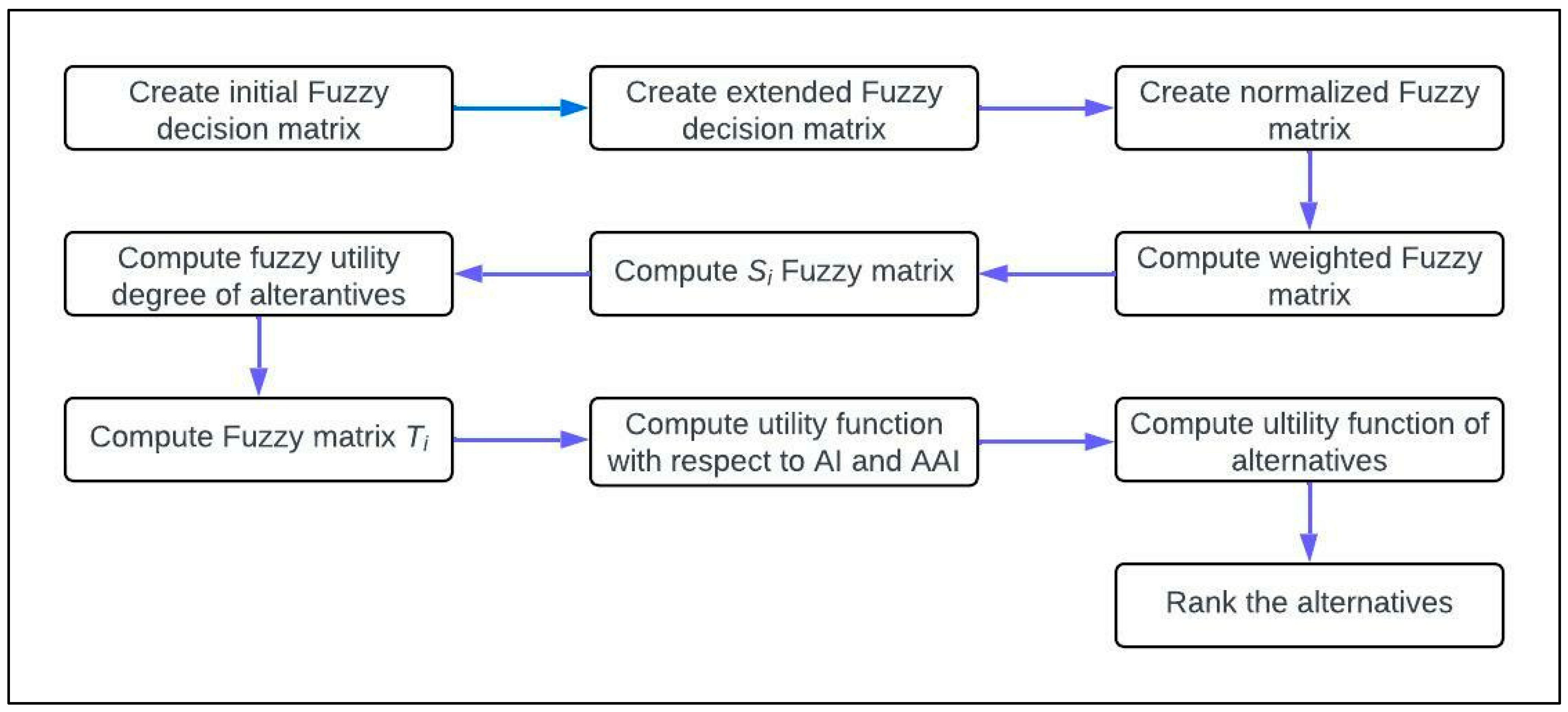
A flowchart describing the process followed in the Fuzzy MARCOS is detailed in Figure 1.
Table 1 shows the fuzzy scale for the analysis, in which nine linguistic terms were defined based on TFNs. This scale will be used for both case studies to analyze the results and rank the alternatives. The worst priority is defined by the linguistic term ‘Extremely poor (EP)’ given by (1,1,1) TFN, while the best priority set is defined by the term ‘Extremely Good, i.e., EG’, and the TFN given to it is (7,9,9).
3. Case Study 1: Green Dry Milling of SS 304 Steel
3.1. Problem Description
The experimental data for the current work are taken from the previously published work by Nguyen et al. [22]. They used a computer numerical control Spinner U620 machining center for the milling of SS304 steel in dry conditions with dimensions 350 mm × 150 mm × 25 mm. The process parameters for the operations were feed rate (), node radius (), depth of cut (), and cutting speed (). During the experiments, three levels of each parameter were selected. For the planning of experiments, 25 combinations of these parameters were obtained by using a Box–Behnken design. The response variables for the experiments were PF (ratio of active power consumption to the apparent consumption of power during experiments), EC (Electrical energy consumed in KJ), and Ra (Average surface roughness in micro-meter). Out of all these three response variables, Ra and EC were analyzed considering the smaller-the-better approach while in the case of PF, lager-the-better was considered ideal. Table 2 shows the experimental plan for the current work along with the output obtained after the experiments for each response.
3.2. Discussion
To apply fuzzy MARCOS to the experiments, weightage for different criteria is given according to four different experts. It should be noted here that the experts assign the criteria importance based on their understanding and opinion on the problem. Thus, it is often possible that all linguistic terms in the fuzzy scale may not be covered in their assigned linguistic weights. For example, in Table 3, EP, VP, and EG linguistic terms do not appear as no expert has assigned them to any of the criteria.
These weights are shown in Table 3 based on the TFNs. Expert 1 gives the most importance to PF and the least importance to EC. According to the 2nd expert, highest priority is given to EC and lowest to Ra, while for the 3rd and 4th experts, PF is most important but Ra is least important for the former while the latter has given the same importance to EC and Ra.
Based on the aggregation of the TFNs for each of the criteria for all the experts, the following fuzzy weights are obtained—(6,6.5,8), (4,5,6), and (3,4.5,5) for PF, EC, and Ra, respectively.
The normalization of the extended fuzzy decision matrix is done using Equations (14) and (15). However, in this case, since the initial decision matrix data in Table 2 is crisp data, the normalization is done using Equations (5) and (6). A sample calculation of the normalized values is shown below for the A1 alternative—
Next, the fuzzy weighted normalized decision matrix is constructed by using Equation (16). A sample calculation of the fuzzy weighted normalized values is shown below for A1 alternative—
Next, the value of was obtained by the summation of the TFNs for each alternative. A sample calculation of value is shown below for the A1 alternative—
Table 4 shows the normalized fuzzy matrix and the value of for each alternative.
Similarly, for the value of of AI, the following calculation is shown,
In Table 5, utility degrees and utility functions are calculated for each alternative using Equations (17)–(21). Sample calculations for the A1 alternative are shown below—
Next, the fuzzy matrix is computed as
Following this, the fuzzy number is computed from fuzzy matrix and subsequently the is computed.
Sample calculation for A1 alternative for and are as follows,
After obtaining the utility degree and the utility function for each alternative defuzzification of the utility function, the utility degree for the ideal as well as the anti-ideal solution is done. The defuzzified value of utility degree and function along with the final ranking of the alternatives is given in Table 6. Sample calculations for the A1 alternative are shown below,
After applying the complete fuzzy MARCOS methodology, the given data for green machining of SS 304 alternative 22 were the best alternative for the experiments. This suggests that a cutting speed of 160 m/min, 0.6 mm depth of cut, 0.08 mm/s feed, and nose radius of 0.8 mm was the best combination for the operation. This combination had 0.862 PF, 26.68 kJ of the utilization of electrical energy, and produced a surface roughness of 0.36 . Alternative 17 was provided with the least rank by the complete analysis. From the analysis, we can say that a combination of = 60 m/min, = 0.6 mm, = 0.04 mm/s, and = 0.4 mm which have a PF ratio of 0.529, consumes 94.95 kJ of electrical energy and produces 0.82 surface roughness.
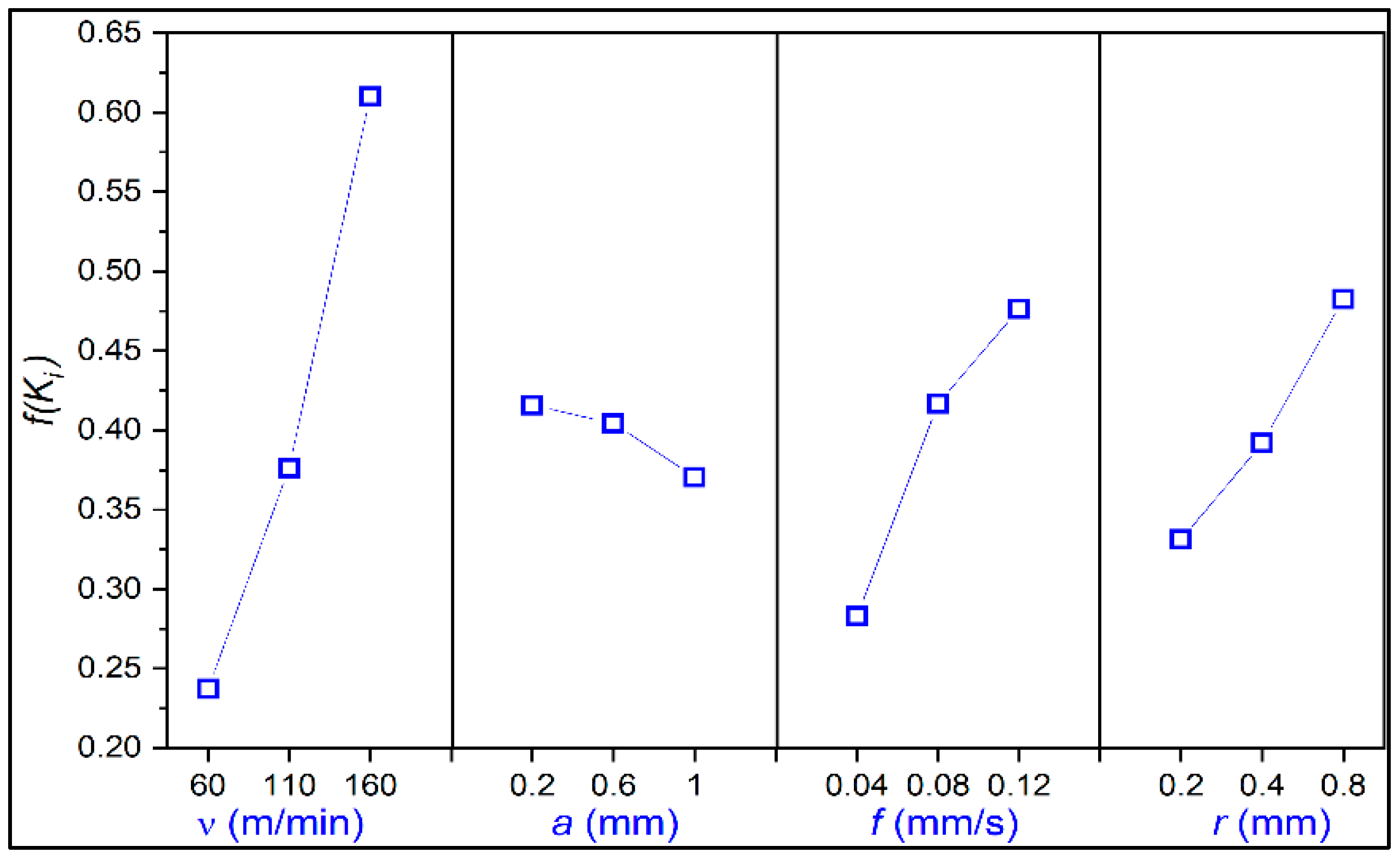
Level-wise aggregation is applied for each of the four process parameters and the corresponding is computed. As shown in Figure 2, this helps in identifying the most suitable level for each process parameter. For Figure 2, it can be summarized that on an aggregated level, = 160 m/min, = 0.2 mm, = 0.12 mm/s, and = 0.8 mm is most suitable.
The obtained results are compared with existing solutions from the literature and reported in Table 7. Since for the obtained parametric combination, the experimental values are not available, the corresponding response values are calculated by using the mathematical equations presented by Das and Chakraborty [23]. It should be noted that the response values reported by Das and Chakraborty [23] are calculated by the same mathematical equations. From Table 7, it is observed that the current solutions are better than those in the literature, especially for PF response.
4. Case Study 2: Green Face Milling of AISI 1045 Steel
4.1. Problem Description
The experimental data for the current work are taken from the previously published work by Khan et al. [24]. They used a computer numerical control Spinner U620 machining center for the milling of AISI 1045 steel in dry condition. The process parameters for the operations were feed rate (), width of cut (), depth of cut (), and cutting speed (). during the experiments, three levels of each parameter were selected as shown in Table 8. For the planning of experiments, 27 combinations of these parameters were obtained by using Taguchi’s orthogonal design. The response variables for the experiments were MRR, ACE, and Ra. Out of all these three response variables, Ra and EC were analyzed considering smaller-the-better approach while for MRR lager-the-better was considered ideal. Table 8 shows the experimental plan for the current work along with the output obtained after the experiments for each response.
4.2. Discussion
To apply fuzzy MARCOS to experiments weightage for different criteria is given according to four different experts. These weights are shown in Table 9 based on the TFNs. According to 1st and 2nd experts, MRR (EG and VG, respectively) is the most important but the former gives the least importance which is the same for Ra and ACE (MP) while the latter gives the least to ACE (MG). According to expert 3, most important is MRR and ACE (G) and the least important is Ra (MG). According to the 4th expert, highest priority is allocated to MRR (G) and the lowest to ACE (P).
After assigning the weightage according to the fuzzy scale to each criterion, a fuzzy normalized matrix is created, which is followed by the calculation of the utility degree and the utility function for each alternative along with the values based on ideal and anti-ideal solutions using Equations (14)–(21). After obtaining the utility degree and the utility function for each alternative defuzzification of the utility function, the utility degree for the ideal as well as the anti-ideal solution is done. The defuzzified value of utility degree and function along with the final ranking of the alternatives is given in Table 10.
After applying the complete fuzzy MARCOS methodology, the given data for green machining of AISI 1045 alternative 9 was the best alternative for the experiments. This suggests that a cutting speed () of 1200 rev/min, 0.5 mm depth of cut (), 320 mm/min feed rate (), and width of cut () of 15 mm was the best combination for the operation. This combination has MRR of 2400 , produces the surface roughness (Ra) of 2.29 , and utilizes 53.988 kJ active cutting energy (ACE). Alternative 1 was given the lowest rank by the complete analysis. From the analysis, we can say that combination of = 1200 rev/min, = 0.3 mm, = 220 mm/min, and = 5 mm which have a MRR of 330 , consumes 535.802 kJ of active cutting energy (ACE) and produces 3.3 surface roughness (Ra).
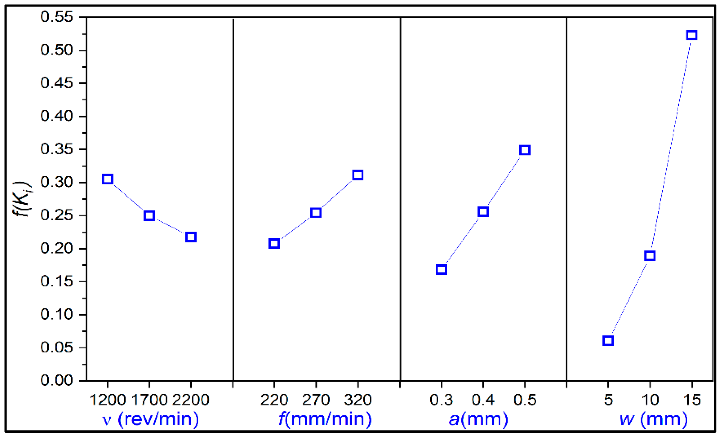
Level-wise aggregation is applied for each of the four process parameters and the corresponding is computed. From Figure 3, it is seen that on an aggregated level, = 1200 rev/min, = 320 mm/min, = 0.5 mm, and = 15 mm is most suitable.
The obtained results are compared with existing solutions from the literature. It should be noted that the optimal combination suggested by the current Fuzzy MARCOS is in exact sync with the results presented by Khan et al. [24]. Thus, a low cutting speed is accompanied by a high feed rate. In terms of the mechanics of the milling process, it is already understood from various works [23,24] that lower cutting speed generally provides better surface quality and consumes minimum active energy.
5. Conclusions
The current work shows the application of the Fuzzy MARCOS method for the optimization of process parameters for the green machining of two different materials, i.e., SS 304 and AISI 1045 at different machining parameters and different responses. After analyzing the process, the following conclusions were drawn:
- The application of the Fuzzy MARCOS method does not follow a rigid weight allocation. The inclusion of fuzzy provides a linguistic scale to provide the weight for the criterion based on different fuzzy numbers; here we used triangular fuzzy numbers, which divided the scale into 9 parts. This allowed us to analyze the problem more practically.
- From the analysis, it is found that for the machining of SS 304 in case study 1 alternative 22 was the best alternative for the experiments. This suggests that a cutting speed of 160 m/min, 0.6 mm depth of cut, 0.08 mm/s feed, and nose radius of 0.8 mm was the best combination for the operation. This combination has a power factor (PF) of 0.862, 26.68 kJ of utilization of electrical energy, and produces a surface roughness of 0.36 .
- If we consider the worst alternative for the 1st case study, alternative 17 was given the lowest rank by the complete analysis. From the analysis, we can say that a combination of = 60 m/min, = 0.6 mm, = 0.04 mm/s, and r = 0.4 mm which have a PF ratio of 0.529, consumes 94.95 kJ of electrical energy, and produces 0.82 surface roughness.
- In the case of the second case study for the green machining of AISI 1045, alternative 9 was the best alternative for the experiments. This suggests that a cutting speed () of 1200 rev/min, 0.5 mm depth of cut (), 320 mm/min feed rate (), and width of cut () of 15 mm was the best combination for the operation. This combination has MRR of 2400 , produces the surface roughness (Ra) of 2.29 , and utilizes 53.988 kJ active cutting energy (ACE).
- Alternative 1 was provided with the lowest rank by the complete analysis for the green machining of AISI 1045. From the analysis, we can say that combination of = 1200 rev/min, = 0.3 mm, = 220 mm/min, and = 5 mm has a MRR of 330 , consumes 535.802 kJ of active cutting energy (ACE), and produces 3.3 surface roughness (Ra).
- Thus, Fuzzy MARCOS is seen to be a powerful technique that combines the uncertainty analysis component and group decision-making ability of fuzzification with the superb selection capability of MARCOS. The method is however limited by its complexity as compared to vanilla MARCOS. Moreover, the fuzzy MARCOS needs several additional calculations which makes it relatively more time intensive. Nevertheless, it is expected that fuzzy MARCOS will become a preferred tool among MCDM specialists, especially due to the remarkable success vanilla MARCOS has had in recent times. This study can be further extended to incorporate various other fuzzy numbers and theories such as interval fuzzy, intuitionistic fuzzy, etc.
Author Contributions
Conceptualization, G.S., T.K.M., R.Č. and K.K.; formal analysis, G.S. and T.K.M.; investigation, G.S. and T.K.M.; methodology, G.S., T.K.M., R.Č. and K.K.; software, R.Č. and K.K.; writing—original draft, G.S. and T.K.M.; writing—review and editing, R.Č. and K.K. All authors have read and agreed to the published version of the manuscript.
Funding
This research received no external funding.
Institutional Review Board Statement
Not applicable.
Informed Consent Statement
Not applicable.
Data Availability Statement
The data presented in this study are available in the article.
Conflicts of Interest
The authors declare no conflict of interest.
References
- Krolczyk, G.M.; Maruda, R.W.; Krolczyk, J.B.; Wojciechowski, S.; Mia, M.; Nieslony, P.; Budzik, G. Ecological Trends in Machining as a Key Factor in Sustainable Production—A Review. J. Clean. Prod. 2019, 218, 601–615. [Google Scholar] [CrossRef]
- Khanna, N.; Shah, P.; Sarikaya, M.; Pusavec, F. Energy Consumption and Ecological Analysis of Sustainable and Conventional Cutting Fluid Strategies in Machining 15–5 PHSS. Sustain. Mater. Technol. 2022, 32, e00416. [Google Scholar] [CrossRef]
- Nouioua, M.; Laouissi, A.; Brahami, R.; Blaoui, M.M.; Hammoudi, A.; Yallese, M.A. Evaluation Of: MOSSA, MOALO, MOVO and MOGWO Algorithms in Green Machining to Enhance the Turning Performances of X210Cr12 Steel. Int. J. Adv. Manuf. Technol. 2022, 120, 2135–2150. [Google Scholar] [CrossRef]
- Kadam, G.S.; Pawade, R.S. Comparative Assessment of Machining Induced Hardening in HSM of Inconel 718 with Aid of Eco-Friendly Cutting Fluids. Mater. Today: Proc. 2022, 62, 7528–7533. [Google Scholar] [CrossRef]
- Bibin, C.; Devarajan, Y.; Bharadwaj, A.; Patil, P.Y. Detailed Analysis on Nonedible Waste Feedstock as a Renewable Cutting Fluid for a Sustainable Machining Process. Biomass Convers. Biorefinery 2022, 1–9. [Google Scholar] [CrossRef]
- Baroi, B.K.; Jagadish; Patowari, P.K. A Review on Sustainability, Health, and Safety Issues of Electrical Discharge Machining. J. Braz. Soc. Mech. Sci. Eng. 2022, 44, 59. [Google Scholar] [CrossRef]
- Sanmotra, H.; Mishra, V.; Gangwar, S.; Singh, G.; Singh, R.; Garg, H.; Karar, V. Feasibility Study on Machining of Niobium to Achieve Nanometric Surface Finish. Lecture Notes in Mechanical Engineering; In Advances in Materials Processing; Springer: Singapore, Singapore, 2020; pp. 301–311. [Google Scholar] [CrossRef]
- Airao, J.; Nirala, C.K.; Bertolini, R.; Krolczyk, G.M.; Khanna, N. Sustainable Cooling Strategies to Reduce Tool Wear, Power Consumption and Surface Roughness during Ultrasonic Assisted Turning of Ti-6Al-4V. Tribol. Int. 2022, 169, 107494. [Google Scholar] [CrossRef]
- Kulisz, M.; Zagórski, I.; Weremczuk, A.; Rusinek, R.; Korpysa, J. Analysis and Prediction of the Impact of Technological Parameters on Cutting Force Components in Rough Milling of AZ31 Magnesium Alloy. Arch. Civ. Mech. Eng. 2021, 22, 1. [Google Scholar] [CrossRef]
- Liu, X.; Han, L.; Wu, S.; Meng, Y.; Yue, C.; Liang, S.Y. Influence of Blade Curvature Characteristics on Energy Consumption in Machining Process. Int. J. Adv. Manuf. Technol. 2022, 121, 1867–1885. [Google Scholar] [CrossRef]
- Wu, P.; He, Y.; Li, Y.; He, J.; Liu, X.; Wang, Y. Multi-Objective Optimisation of Machining Process Parameters Using Deep Learning-Based Data-Driven Genetic Algorithm and TOPSIS. J. Manuf. Syst. 2022, 64, 40–52. [Google Scholar] [CrossRef]
- EKİCİ, E.; UZUN, G. Effects on Machinability of Cryogenic Treatment Applied to Carbide Tools in the Milling of Ti6AI4V with Optimization via the Taguchi Method and Grey Relational Analysis. J. Braz. Soc. Mech. Sci. Eng. 2022, 44, 270. [Google Scholar] [CrossRef]
- Kumar, R.; Katyal, P.; Kumar, K.; Singh, V. Multiresponse Optimization of End Milling Process Parameters on ZE41A Mg Alloy Using Taguchi and TOPSIS Approach. Mater. Today Proc. 2021, 56, 2497–2504. [Google Scholar] [CrossRef]
- Safi, K.; Yallese, M.A.; Belhadi, S.; Mabrouki, T.; Laouissi, A. Tool Wear, 3D Surface Topography, and Comparative Analysis of GRA, MOORA, DEAR, and WASPAS Optimization Techniques in Turning of Cold Work Tool Steel. Int. J. Adv. Manuf. Technol. 2022, 121, 701–721. [Google Scholar] [CrossRef]
- Singh, T.; Sharma, V.K.; Rana, M.; Singh, K.; Saini, A. GRA Based Optimization of Tool Vibration and Surface Roughness in Face Milling of Hardened Steel Alloy. Mater. Today Proc. 2022, 50, 2288–2293. [Google Scholar] [CrossRef]
- Zheng, Q.; Chen, G.; Jiao, A. Chatter Detection in Milling Process Based on the Combination of Wavelet Packet Transform and PSO-SVM. Int. J. Adv. Manuf. Technol. 2022, 120, 1237–1251. [Google Scholar] [CrossRef]
- Stanković, M.; Stević, Ž.; Das, D.K.; Subotić, M.; Pamučar, D. A New Fuzzy MARCOS Method for Road Traffic Risk Analysis. Mathematics 2020, 8, 457. [Google Scholar] [CrossRef] [Green Version]
- Taş, M.A.; Çakır, E.; Ulukan, Z. Spherical Fuzzy SWARA-MARCOS Approach for Green Supplier Selection. 3C Tecnol. Glosas Innovación Apl. Pyme 2021, 10, 115–133. [Google Scholar] [CrossRef]
- Ali, J. A Q-Rung Orthopair Fuzzy MARCOS Method Using Novel Score Function and Its Application to Solid Waste Management. Appl. Intell. 2021, 52, 8770–8792. [Google Scholar] [CrossRef]
- Bakır, M.; Atalık, Ö. Application of Fuzzy AHP and Fuzzy MARCOS Approach for the Evaluation of E-Service Quality in the Airline Industry. Decis. Mak. Appl. Manag. Eng. 2021, 4, 127–152. [Google Scholar] [CrossRef]
- Kovač, M.; Tadić, S.; Krstić, M.; Bouraima, M.B. Novel Spherical Fuzzy MARCOS Method for Assessment of Drone-Based City Logistics Concepts. Complexity 2021, 2021, 2374955. [Google Scholar] [CrossRef]
- Nguyen, T.-T.; Nguyen, T.-A.; Trinh, Q.-H. Optimization of Milling Parameters for Energy Savings and Surface Quality. Arab. J. Sci. Eng. 2020, 45, 9111–9125. [Google Scholar] [CrossRef]
- Das, P.P.; Chakraborty, S. SWARA-CoCoSo Method-Based Parametric Optimization of Green Dry Milling Processes. J. Eng. Appl. Sci. 2022, 69, 35. [Google Scholar] [CrossRef]
- Khan, A.; Jamil, M.; Salonitis, K.; Sarfraz, S.; Zhao, W.; He, N.; Mia, M.; Zhao, G. Multi-Objective Optimization of Energy Consumption and Surface Quality in Nanofluid SQCL Assisted Face Milling. Energies 2019, 12, 710. [Google Scholar] [CrossRef]
Figure 1.
Flowchart of Fuzzy MARCOS method.

Figure 2.
Level-wise aggregated f (K_i) score for each process parameter.

Figure 3.
Level-wise aggregated f(K_i) score for each process parameter in case study 2.


Table 1.
Fuzzy scale used in the study.
| Linguistic Term for Importance of Criteria | Symbol | Triangular Fuzzy Number |
|---|---|---|
| Extremely Poor | EP | (1,1,1) |
| Very Poor | VP | (1,1,3) |
| Poor | P | (1,3,3) |
| Medium Poor | MP | (3,3,5) |
| Medium | M | (3,5,5) |
| Medium Good | MG | (5,5,7) |
| Good | G | (5,7,7) |
| Very Good | VG | (7,7,9) |
| Extremely Good | EG | (7,9,9) |
Table 2.
Experimental dataset on green dry milling of SS 304 steel (case study 1) [22].
Table 2.
Experimental dataset on green dry milling of SS 304 steel (case study 1) [22].
| Exp.no. | PF | EC (kJ) | |||||
|---|---|---|---|---|---|---|---|
| 1 | 110 | 0.2 | 0.04 | 0.4 | 0.518 | 50.33 | 0.45 |
| 2 | 110 | 0.6 | 0.12 | 0.8 | 0.867 | 25.46 | 1.08 |
| 3 | 110 | 0.6 | 0.08 | 0.4 | 0.652 | 31.56 | 0.85 |
| 4 | 60 | 0.6 | 0.08 | 0.2 | 0.611 | 53.66 | 1.34 |
| 5 | 160 | 0.6 | 0.12 | 0.4 | 0.851 | 18.42 | 0.95 |
| 6 | 60 | 0.6 | 0.12 | 0.4 | 0.736 | 42.6 | 1.47 |
| 7 | 110 | 0.2 | 0.12 | 0.4 | 0.69 | 21.99 | 1.14 |
| 8 | 60 | 0.6 | 0.08 | 0.8 | 0.685 | 59.13 | 0.78 |
| 9 | 60 | 1 | 0.08 | 0.4 | 0.703 | 61.68 | 1.31 |
| 10 | 110 | 1 | 0.12 | 0.4 | 0.868 | 26.72 | 1.49 |
| 11 | 110 | 1 | 0.08 | 0.2 | 0.732 | 35.41 | 1.42 |
| 12 | 160 | 0.6 | 0.08 | 0.2 | 0.719 | 22.84 | 0.89 |
| 13 | 160 | 1 | 0.08 | 0.4 | 0.835 | 27.26 | 0.79 |
| 14 | 60 | 0.2 | 0.08 | 0.4 | 0.547 | 48.96 | 0.82 |
| 15 | 160 | 0.6 | 0.04 | 0.4 | 0.69 | 44.62 | 0.47 |
| 16 | 110 | 0.6 | 0.04 | 0.2 | 0.566 | 54.03 | 0.98 |
| 17 | 60 | 0.6 | 0.04 | 0.4 | 0.529 | 94.95 | 0.82 |
| 18 | 110 | 1 | 0.04 | 0.4 | 0.659 | 63.82 | 1.06 |
| 19 | 160 | 0.2 | 0.08 | 0.4 | 0.671 | 22.07 | 0.41 |
| 20 | 110 | 0.6 | 0.12 | 0.2 | 0.752 | 23.74 | 1.55 |
| 21 | 110 | 0.6 | 0.04 | 0.8 | 0.648 | 62.35 | 0.52 |
| 22 | 160 | 0.6 | 0.08 | 0.8 | 0.862 | 26.68 | 0.36 |
| 23 | 110 | 0.2 | 0.08 | 0.2 | 0.576 | 28.23 | 0.91 |
| 24 | 110 | 0.2 | 0.08 | 0.8 | 0.681 | 32.95 | 0.48 |
| 25 | 110 | 1 | 0.08 | 0.8 | 0.843 | 39.02 | 0.89 |
Table 3.
Experimental dataset on green dry milling of SS 304 steel.
| Decision Maker | Linguistic Term | Triangular Fuzzy Number | ||||
|---|---|---|---|---|---|---|
| PF | EC (kJ) | PF | EC (kJ) | |||
| Expert 1 | VG | M | G | (7,7,9) | (3,5,5) | (5,7,7) |
| Expert 2 | MG | G | M | (5,5,7) | (5,7,7) | (3,5,5) |
| Expert 3 | G | MG | P | (5,7,7) | (5,5,7) | (1,3,3) |
| Expert 4 | VG | MP | MP | (7,7,9) | (3,3,5) | (3,3,5) |
Table 4.
Fuzzy weighted normalized decision matrix and values (case study 1).
| Alternative | PF | EC (kJ) | ||
|---|---|---|---|---|
| AAI | (3.5806, 3.879, 4.7742) | (0.776, 0.97, 1.164) | (0.6968, 1.0452, 1.1613) | (5.0534, 5.8942, 7.0995) |
| A1 | (3.5806, 3.879, 4.7742) | (1.4639, 1.8299, 2.1959) | (2.4, 3.6, 4) | (7.4446, 9.309, 10.9701) |
| A2 | (5.9931, 6.4925, 7.9908) | (2.894, 3.6174, 4.3409) | (1, 1.5, 1.6667) | (9.887, 11.61, 13.9984) |
| A3 | (4.5069, 4.8825, 6.0092) | (2.3346, 2.9183, 3.5019) | (1.2706, 1.9059, 2.1176) | (8.1121, 9.7066, 11.6288) |
| A4 | (4.2235, 4.5755, 5.6313) | (1.3731, 1.7164, 2.0596) | (0.806, 1.209, 1.3433) | (6.4026, 7.5008, 9.0343) |
| A5 | (5.8825, 6.3727, 7.8433) | (4, 5, 6) | (1.1368, 1.7053, 1.8947) | (11.0193, 13.078, 15.7381) |
| A6 | (5.0876, 5.5115, 6.7834) | (1.7296, 2.162, 2.5944) | (0.7347, 1.102, 1.2245) | (7.5518, 8.7755, 10.6023) |
| A7 | (4.7696, 5.1671, 6.3594) | (3.3506, 4.1883, 5.0259) | (0.9474, 1.4211, 1.5789) | (9.0676, 10.7764, 12.9643) |
| A8 | (4.735, 5.1296, 6.3134) | (1.2461, 1.5576, 1.8691) | (1.3846, 2.0769, 2.3077) | (7.3657, 8.7641, 10.4902) |
| A9 | (4.8594, 5.2644, 6.4793) | (1.1946, 1.4932, 1.7918) | (0.8244, 1.2366, 1.374) | (6.8784, 7.9942, 9.6451) |
| A10 | (6, 6.5, 8) | (2.7575, 3.4469, 4.1362) | (0.7248, 1.0872, 1.2081) | (9.4823, 11.0341, 13.3443) |
| A11 | (5.0599, 5.4816, 6.7465) | (2.0808, 2.601, 3.1212) | (0.7606, 1.1408, 1.2676) | (7.9012, 9.2234, 11.1353) |
| A12 | (4.97, 5.3842, 6.6267) | (3.2259, 4.0324, 4.8389) | (1.2135, 1.8202, 2.0225) | (9.4094, 11.2368, 13.4881) |
| A13 | (5.7719, 6.2529, 7.6959) | (2.7029, 3.3786, 4.0543) | (1.3671, 2.0506, 2.2785) | (9.8418, 11.6821, 14.0286) |
| A14 | (3.7811, 4.0962, 5.0415) | (1.5049, 1.8811, 2.2574) | (1.3171, 1.9756, 2.1951) | (6.6031, 7.9529, 9.4939) |
| A15 | (4.7696, 5.1671, 6.3594) | (1.6513, 2.0641, 2.4769) | (2.2979, 3.4468, 3.8298) | (8.7187, 10.678, 12.6662) |
| A16 | (3.9124, 4.2385, 5.2166) | (1.3637, 1.7046, 2.0455) | (1.102, 1.6531, 1.8367) | (6.3782, 7.5961, 9.0989) |
| A17 | (3.6567, 3.9614, 4.8756) | (0.776, 0.97, 1.164) | (1.3171, 1.9756, 2.1951) | (5.7497, 6.907, 8.2347) |
| A18 | (4.5553, 4.9349, 6.0737) | (1.1545, 1.4431, 1.7317) | (1.0189, 1.5283, 1.6981) | (6.7287, 7.9063, 9.5036) |
| A19 | (4.6382, 5.0248, 6.1843) | (3.3385, 4.1731, 5.0077) | (2.6341, 3.9512, 4.3902) | (10.6109, 13.1491, 15.5823) |
| A20 | (5.1982, 5.6313, 6.9309) | (3.1036, 3.8795, 4.6554) | (0.6968, 1.0452, 1.1613) | (8.9986, 10.556, 12.7476) |
| A21 | (4.4793, 4.8525, 5.9724) | (1.1817, 1.4771, 1.7726) | (2.0769, 3.1154, 3.4615) | (7.7379, 9.4451, 11.2065) |
| A22 | (5.9585, 6.4551, 7.9447) | (2.7616, 3.452, 4.1424) | (3, 4.5, 5) | (11.7201, 14.4071, 17.0871) |
| A23 | (3.9816, 4.3134, 5.3088) | (2.61, 3.2625, 3.915) | (1.1868, 1.7802, 1.978) | (7.7784, 9.3561, 11.2018) |
| A24 | (4.7074, 5.0997, 6.2765) | (2.2361, 2.7951, 3.3542) | (2.25, 3.375, 3.75) | (9.1935, 11.2698, 13.3807) |
| A25 | (5.8272, 6.3128, 7.7696) | (1.8883, 2.3603, 2.8324) | (1.2135, 1.8202, 2.0225) | (8.9289, 10.4933, 12.6245) |
| AI | (6, 6.5, 8) | (4, 5, 6) | (3, 4.5, 5) | (13, 16, 19) |
Table 5.
Utility degree of alternatives and utility functions (case study 1).
| Alternative | Utility Degree | Utility Functions | ||
|---|---|---|---|---|
| A1 | (1.0486, 1.5793, 2.1708) | (0.3918, 0.5818, 0.8439) | (0.1156, 0.1716, 0.2489) | (0.3093, 0.4658, 0.6403) |
| A2 | (1.3926, 1.9697, 2.7701) | (0.5204, 0.7256, 1.0768) | (0.1535, 0.214, 0.3176) | (0.4108, 0.581, 0.817) |
| A3 | (1.1426, 1.6468, 2.3012) | (0.427, 0.6067, 0.8945) | (0.1259, 0.1789, 0.2638) | (0.337, 0.4857, 0.6787) |
| A4 | (0.9018, 1.2726, 1.7878) | (0.337, 0.4688, 0.6949) | (0.0994, 0.1383, 0.205) | (0.266, 0.3753, 0.5273) |
| A5 | (1.5521, 2.2188, 3.1143) | (0.58, 0.8174, 1.2106) | (0.1711, 0.2411, 0.3571) | (0.4578, 0.6544, 0.9186) |
| A6 | (1.0637, 1.4888, 2.098) | (0.3975, 0.5485, 0.8156) | (0.1172, 0.1618, 0.2406) | (0.3137, 0.4391, 0.6188) |
| A7 | (1.2772, 1.8283, 2.5655) | (0.4772, 0.6735, 0.9973) | (0.1408, 0.1987, 0.2941) | (0.3767, 0.5393, 0.7567) |
| A8 | (1.0375, 1.4869, 2.0759) | (0.3877, 0.5478, 0.8069) | (0.1143, 0.1616, 0.238) | (0.306, 0.4386, 0.6123) |
| A9 | (0.9689, 1.3563, 1.9086) | (0.362, 0.4996, 0.7419) | (0.1068, 0.1474, 0.2188) | (0.2858, 0.4, 0.563) |
| A10 | (1.3356, 1.872, 2.6407) | (0.4991, 0.6896, 1.0265) | (0.1472, 0.2034, 0.3028) | (0.3939, 0.5522, 0.7789) |
| A11 | (1.1129, 1.5648, 2.2035) | (0.4159, 0.5765, 0.8566) | (0.1227, 0.17, 0.2526) | (0.3283, 0.4615, 0.6499) |
| A12 | (1.3254, 1.9064, 2.6691) | (0.4952, 0.7023, 1.0375) | (0.1461, 0.2071, 0.306) | (0.3909, 0.5623, 0.7873) |
| A13 | (1.3863, 1.982, 2.7761) | (0.518, 0.7301, 1.0791) | (0.1528, 0.2154, 0.3183) | (0.4089, 0.5846, 0.8188) |
| A14 | (0.9301, 1.3493, 1.8787) | (0.3475, 0.4971, 0.7303) | (0.1025, 0.1466, 0.2154) | (0.2743, 0.398, 0.5541) |
| A15 | (1.2281, 1.8116, 2.5065) | (0.4589, 0.6674, 0.9743) | (0.1353, 0.1968, 0.2874) | (0.3622, 0.5343, 0.7393) |
| A16 | (0.8984, 1.2888, 1.8005) | (0.3357, 0.4748, 0.6999) | (0.099, 0.14, 0.2064) | (0.265, 0.3801, 0.5311) |
| A17 | (0.8099, 1.1718, 1.6295) | (0.3026, 0.4317, 0.6334) | (0.0893, 0.1273, 0.1868) | (0.2389, 0.3456, 0.4806) |
| A18 | (0.9478, 1.3414, 1.8806) | (0.3541, 0.4941, 0.731) | (0.1045, 0.1457, 0.2156) | (0.2795, 0.3956, 0.5547) |
| A19 | (1.4946, 2.2309, 3.0835) | (0.5585, 0.8218, 1.1986) | (0.1647, 0.2424, 0.3535) | (0.4408, 0.658, 0.9095) |
| A20 | (1.2675, 1.7909, 2.5226) | (0.4736, 0.6598, 0.9806) | (0.1397, 0.1946, 0.2892) | (0.3738, 0.5282, 0.744) |
| A21 | (1.0899, 1.6024, 2.2176) | (0.4073, 0.5903, 0.862) | (0.1201, 0.1741, 0.2543) | (0.3215, 0.4726, 0.6541) |
| A22 | (1.6508, 2.4443, 3.3813) | (0.6168, 0.9004, 1.3144) | (0.1819, 0.2656, 0.3877) | (0.4869, 0.7209, 0.9973) |
| A23 | (1.0956, 1.5873, 2.2167) | (0.4094, 0.5848, 0.8617) | (0.1207, 0.1725, 0.2542) | (0.3232, 0.4682, 0.6538) |
| A24 | (1.295, 1.912, 2.6479) | (0.4839, 0.7044, 1.0293) | (0.1427, 0.2078, 0.3036) | (0.3819, 0.564, 0.781) |
| A25 | (1.2577, 1.7803, 2.4982) | (0.4699, 0.6558, 0.9711) | (0.1386, 0.1934, 0.2864) | (0.371, 0.5251, 0.7368) |
Table 6.
Defuzzied utility degree, utility functions, and ranks of the alternatives (case study 1).
| Alternative | Rank | |||||||
|---|---|---|---|---|---|---|---|---|
| A1 | 1.5895 | 0.5938 | 0.1751 | 0.4688 | 4.7095 | 1.1330 | 0.3191 | 17 |
| A2 | 2.0069 | 0.7499 | 0.2212 | 0.5920 | 3.5209 | 0.6893 | 0.5291 | 5 |
| A3 | 1.6718 | 0.6247 | 0.1843 | 0.4931 | 4.4273 | 1.0279 | 0.3558 | 13 |
| A4 | 1.2966 | 0.4845 | 0.1429 | 0.3824 | 5.9974 | 1.6147 | 0.2068 | 24 |
| A5 | 2.2569 | 0.8433 | 0.2487 | 0.6657 | 3.0202 | 0.5022 | 0.6855 | 2 |
| A6 | 1.5195 | 0.5678 | 0.1675 | 0.4482 | 4.9709 | 1.2312 | 0.2898 | 18 |
| A7 | 1.8593 | 0.6948 | 0.2049 | 0.5484 | 3.8799 | 0.8235 | 0.4478 | 9 |
| A8 | 1.5102 | 0.5643 | 0.1664 | 0.4454 | 5.0084 | 1.2450 | 0.2860 | 19 |
| A9 | 1.3838 | 0.5171 | 0.1525 | 0.4081 | 5.5567 | 1.4501 | 0.2374 | 20 |
| A10 | 1.9107 | 0.7140 | 0.2106 | 0.5636 | 3.7484 | 0.7744 | 0.4753 | 8 |
| A11 | 1.5960 | 0.5964 | 0.1759 | 0.4707 | 4.6850 | 1.1244 | 0.3220 | 16 |
| A12 | 1.9367 | 0.7237 | 0.2134 | 0.5712 | 3.6850 | 0.7506 | 0.4894 | 6 |
| A13 | 2.0150 | 0.7529 | 0.2221 | 0.5943 | 3.5029 | 0.6825 | 0.5338 | 4 |
| A14 | 1.3677 | 0.5110 | 0.1507 | 0.4034 | 5.6347 | 1.4790 | 0.2315 | 21 |
| A15 | 1.8302 | 0.6838 | 0.2017 | 0.5398 | 3.9583 | 0.8525 | 0.4326 | 10 |
| A16 | 1.3090 | 0.4891 | 0.1443 | 0.3861 | 5.9318 | 1.5901 | 0.2110 | 23 |
| A17 | 1.1878 | 0.4438 | 0.1309 | 0.3503 | 6.6394 | 1.8544 | 0.1719 | 25 |
| A18 | 1.3657 | 0.5103 | 0.1505 | 0.4028 | 5.6440 | 1.4826 | 0.2308 | 22 |
| A19 | 2.2503 | 0.8407 | 0.2480 | 0.6637 | 3.0327 | 0.5067 | 0.6809 | 3 |
| A20 | 1.8256 | 0.6822 | 0.2012 | 0.5385 | 3.9698 | 0.8571 | 0.4304 | 11 |
| A21 | 1.6195 | 0.6051 | 0.1785 | 0.4777 | 4.6031 | 1.0934 | 0.3322 | 14 |
| A22 | 2.4682 | 0.9222 | 0.2720 | 0.7280 | 2.6765 | 0.3736 | 0.8371 | 1 |
| A23 | 1.6103 | 0.6017 | 0.1775 | 0.4750 | 4.6349 | 1.1055 | 0.3282 | 15 |
| A24 | 1.9318 | 0.7218 | 0.2129 | 0.5698 | 3.6974 | 0.7550 | 0.4867 | 7 |
| A25 | 1.8128 | 0.6774 | 0.1998 | 0.5347 | 4.0050 | 0.8702 | 0.4239 | 12 |
Table 7.
Comparison with results from literature.
| Source | PF | EC (kJ) | Average | |||||
|---|---|---|---|---|---|---|---|---|
| Current | 160 | 0.2 | 0.12 | 0.8 | 0.9908 | 23.2264 | 0.2949 | - |
| Nguyen et al. [22] | 160 | 0.42 | 0.09 | 0.8 | 0.8360 | 20.6300 | 0.3500 | - |
| % Improvement | - | - | - | - | 18.52% | −12.59% | 15.74% | 7.22% |
| Das and Chakraborty [23] | 160 | 1 | 0.08 | 0.8 | 0.9830 | 19.9288 | 0.3921 | - |
| % Improvement | - | - | - | - | 0.79% | −16.55% | 24.79% | 3.01% |
| Das and Chakraborty [23] | 160 | 0.2 | 0.08 | 0.8 | 0.8695 | 19.9288 | 0.2947 | - |
| % Improvement | - | - | - | - | 13.95% | −16.55% | −0.07% | −0.89% |
Table 8.
Experimental dataset on green dry milling of AISI 1045 steel (case study 2) [24].
Table 8.
Experimental dataset on green dry milling of AISI 1045 steel (case study 2) [24].
| Exp.no. | ACE (kJ) | ||||||
|---|---|---|---|---|---|---|---|
| 1 | 1200 | 220 | 0.3 | 5 | 330 | 3.3 | 535.802 |
| 2 | 1200 | 220 | 0.4 | 10 | 880 | 2.95 | 184.929 |
| 3 | 1200 | 220 | 0.5 | 15 | 1650 | 1.41 | 88.519 |
| 4 | 1200 | 270 | 0.3 | 5 | 405 | 3.83 | 426.109 |
| 5 | 1200 | 270 | 0.4 | 10 | 1080 | 3.87 | 146.05 |
| 6 | 1200 | 270 | 0.5 | 15 | 2025 | 1.68 | 69.823 |
| 7 | 1200 | 320 | 0.3 | 5 | 480 | 3.97 | 361.832 |
| 8 | 1200 | 320 | 0.4 | 10 | 1280 | 3.53 | 122.976 |
| 9 | 1200 | 320 | 0.5 | 15 | 2400 | 2.29 | 53.988 |
| 10 | 1700 | 220 | 0.3 | 10 | 660 | 1.81 | 337.042 |
| 11 | 1700 | 220 | 0.4 | 15 | 1320 | 1.13 | 142.727 |
| 12 | 1700 | 220 | 0.5 | 5 | 550 | 3.47 | 299.031 |
| 13 | 1700 | 270 | 0.3 | 10 | 810 | 2.85 | 269.604 |
| 14 | 1700 | 270 | 0.4 | 15 | 1620 | 1.41 | 113.648 |
| 15 | 1700 | 270 | 0.5 | 5 | 675 | 3.91 | 238.476 |
| 16 | 1700 | 320 | 0.3 | 10 | 960 | 2.55 | 213.559 |
| 17 | 1700 | 320 | 0.4 | 15 | 1920 | 1.39 | 92.551 |
| 18 | 1700 | 320 | 0.5 | 5 | 800 | 4.12 | 193.109 |
| 19 | 2200 | 220 | 0.3 | 15 | 990 | 1.76 | 244.303 |
| 20 | 2200 | 220 | 0.4 | 5 | 440 | 3.33 | 425.797 |
| 21 | 2200 | 220 | 0.5 | 10 | 1100 | 2.36 | 165.62 |
| 22 | 2200 | 270 | 0.3 | 15 | 1215 | 1.17 | 193.939 |
| 23 | 2200 | 270 | 0.4 | 5 | 540 | 3.72 | 338.579 |
| 24 | 2200 | 270 | 0.5 | 10 | 1350 | 2.58 | 131.343 |
| 25 | 2200 | 320 | 0.3 | 15 | 1440 | 1.41 | 160.886 |
| 26 | 2200 | 320 | 0.4 | 5 | 640 | 3.86 | 286.85 |
| 27 | 2200 | 320 | 0.5 | 10 | 1600 | 2.76 | 108.147 |
Table 9.
Experimental dataset on green dry milling of AISI 1045 steel (case study 2).
| Decision Maker | Linguistic Term | Triangular Fuzzy Number | ||||
|---|---|---|---|---|---|---|
| ACE (kJ) | ACE (kJ) | |||||
| Expert 1 | EG | MP | MP | (7,9,9) | (3,3,5) | (3,3,5) |
| Expert 2 | VG | G | MG | (7,7,9) | (5,7,7) | (5,5,7) |
| Expert 3 | G | MG | G | (5,7,7) | (5,5,7) | (5,7,7) |
| Expert 4 | G | MG | P | (5,7,7) | (5,5,7) | (1,3,3) |
Table 10.
Defuzzied utility degree, utility functions, and ranks of the alternatives (case study 2).
Table 10.
Defuzzied utility degree, utility functions, and ranks of the alternatives (case study 2).
| Alternative | ||||||||
|---|---|---|---|---|---|---|---|---|
| A1 | 1.1462 | 0.1942 | 0.0326 | 0.1922 | 29.7081 | 4.2033 | 0.0384 | 27 |
| A2 | 2.1212 | 0.3594 | 0.0603 | 0.3557 | 15.5956 | 1.8116 | 0.1348 | 16 |
| A3 | 4.2299 | 0.7166 | 0.1202 | 0.7093 | 7.3221 | 0.4099 | 0.5665 | 4 |
| A4 | 1.1818 | 0.2002 | 0.0336 | 0.1982 | 28.7837 | 4.0463 | 0.0409 | 26 |
| A5 | 2.2947 | 0.3887 | 0.0652 | 0.3848 | 14.3419 | 1.5990 | 0.1584 | 14 |
| A6 | 4.6603 | 0.7895 | 0.1324 | 0.7814 | 6.5540 | 0.2797 | 0.6957 | 2 |
| A7 | 1.2798 | 0.2168 | 0.0364 | 0.2146 | 26.5041 | 3.6599 | 0.0480 | 25 |
| A8 | 2.6735 | 0.4529 | 0.0759 | 0.4483 | 12.1684 | 1.2307 | 0.2171 | 11 |
| A9 | 5.0999 | 0.8639 | 0.1449 | 0.8551 | 5.9032 | 0.1694 | 0.8432 | 1 |
| A10 | 2.1151 | 0.3584 | 0.0601 | 0.3547 | 15.6407 | 1.8196 | 0.1340 | 17 |
| A11 | 3.8667 | 0.6552 | 0.1099 | 0.6484 | 8.1028 | 0.5423 | 0.4688 | 6 |
| A12 | 1.4809 | 0.2509 | 0.0421 | 0.2483 | 22.7699 | 3.0272 | 0.0646 | 22 |
| A13 | 1.9234 | 0.3259 | 0.0546 | 0.3225 | 17.3014 | 2.1006 | 0.1102 | 18 |
| A14 | 3.9816 | 0.6746 | 0.1131 | 0.6676 | 7.8409 | 0.4978 | 0.4986 | 5 |
| A15 | 1.6221 | 0.2748 | 0.0461 | 0.2720 | 20.7012 | 2.6765 | 0.0778 | 20 |
| A16 | 2.2552 | 0.3821 | 0.0641 | 0.3782 | 14.6088 | 1.6444 | 0.1529 | 15 |
| A17 | 4.5004 | 0.7624 | 0.1278 | 0.7546 | 6.8221 | 0.3252 | 0.6460 | 3 |
| A18 | 1.8153 | 0.3075 | 0.0516 | 0.3044 | 18.3922 | 2.2852 | 0.0979 | 19 |
| A19 | 2.6017 | 0.4408 | 0.0739 | 0.4362 | 12.5296 | 1.2923 | 0.2053 | 12 |
| A20 | 1.3011 | 0.2204 | 0.0370 | 0.2182 | 26.0535 | 3.5838 | 0.0497 | 24 |
| A21 | 2.5891 | 0.4386 | 0.0736 | 0.4341 | 12.5961 | 1.3034 | 0.2032 | 13 |
| A22 | 3.5307 | 0.5982 | 0.1003 | 0.5920 | 8.9692 | 0.6891 | 0.3874 | 8 |
| A23 | 1.3962 | 0.2365 | 0.0397 | 0.2341 | 24.2122 | 3.2716 | 0.0573 | 23 |
| A24 | 2.9206 | 0.4948 | 0.0830 | 0.4897 | 11.0536 | 1.0420 | 0.2608 | 10 |
| A25 | 3.5638 | 0.6038 | 0.1012 | 0.5976 | 8.8771 | 0.6734 | 0.3950 | 7 |
| A26 | 1.5301 | 0.2592 | 0.0435 | 0.2566 | 22.0067 | 2.8977 | 0.0691 | 21 |
| A27 | 3.2795 | 0.5556 | 0.0932 | 0.5499 | 9.7348 | 0.8185 | 0.3320 | 9 |
Publisher’s Note: MDPI stays neutral with regard to jurisdictional claims in published maps and institutional affiliations. |
© 2022 by the authors. Licensee MDPI, Basel, Switzerland. This article is an open access article distributed under the terms and conditions of the Creative Commons Attribution (CC BY) license (https://creativecommons.org/licenses/by/4.0/).
Share and Cite
MDPI and ACS Style
Shanmugasundar, G.; Mahanta, T.K.; Čep, R.; Kalita, K. Novel Fuzzy Measurement Alternatives and Ranking according to the Compromise Solution-Based Green Machining Optimization. Processes 2022, 10, 2645. https://doi.org/10.3390/pr10122645
AMA Style
Shanmugasundar G, Mahanta TK, Čep R, Kalita K. Novel Fuzzy Measurement Alternatives and Ranking according to the Compromise Solution-Based Green Machining Optimization. Processes. 2022; 10(12):2645. https://doi.org/10.3390/pr10122645
Chicago/Turabian StyleShanmugasundar, G., Tapan K. Mahanta, Robert Čep, and Kanak Kalita. 2022. "Novel Fuzzy Measurement Alternatives and Ranking according to the Compromise Solution-Based Green Machining Optimization" Processes 10, no. 12: 2645. https://doi.org/10.3390/pr10122645
Note that from the first issue of 2016, this journal uses article numbers instead of page numbers. See further details here.