Deep Learning Based Target Tracking Algorithm Model for Athlete Training Trajectory

Abstract

The main function of the athlete tracking system is to collect the real-time competition data of the athletes. Deep learning is a research hotspot in the field of image and video. With the rapid development of science and technology, it has not only made a breakthrough in theory, but also achieved excellent results in practical application. SiamRPN (Siamese Region Proposal Network) is a single target tracking network model based on deep learning, which has high accuracy and fast operation speed. However, in long-term tracking, if the target is completely obscured and out of the sight of SiamRPN, the tracking of the network will be invalid. Considering the difficulty of long-term tracking, the algorithm is improved and tested by introducing channel attention mechanism and local global search strategy into SiamRPN. Experimental results show that this algorithm has higher accuracy and prediction average overlap rate than the original SiamRPN algorithm when performing tracking tasks on long-term tracking sequences. At the same time, the improved algorithm can still achieve good results in the case of target disappearance and other challenging factors. This study provides an important reference for the coaches of deep learning to realize long-term tracking of athletes.

1. Introduction

With the improvement of social and economic level and people’s growing demand for spiritual culture, people attach more and more importance to sports events. Therefore, the related applications of sports events have developed rapidly [1]. In a high-quality sports event, real-time acquisition of athletes’ competition information plays a decisive role in coaches’ personnel arrangement and tactical arrangement. However, nowadays, commonly used wearable GPS devices are very complex to operate, difficult to maintain, and it is difficult to ensure accuracy in long-term tracking [2]. With the development of science and technology, tracking technology has also been significantly improved. As the strongest single target tracking algorithm, SiamRPN (Siamese Region Proposal Network) algorithm can better use data to enhance the discrimination ability of tracking target, and solve the problem of conventional tracking technology being unable to use deep neural networks, and improve the accuracy of the model [3]. However, the general SiamRPN algorithm has two problems, one is the problem of adapting to the change of tracking target in the tracking process, and the other is the widespread problem of tracking target disappearing or being occluded in long-term tracking [4]. In order to solve the problems existing in the conventional SiamRPN algorithm and achieve efficient and accurate tracking results, the channel attention mechanism and a simple search strategy from local to global without parameters are introduced, and the SiamRPN algorithm is improved, so as to build a target long-term tracking algorithm model based on deep learning. An excellent target tracking model can meet both accuracy andreal-time requirements, achievingan excellent tracking function for athletes, so that coaches can quickly obtain effective information and complete strategic deployment.

In previous research on single target tracking, there is a lack of related research on long-term tracking. Therefore, the innovation of the research is to improve the SiamRPN tracking algorithm, introduce a local-to-global search strategy to change short-term tracking into long-term tracking, and then add channel attention mechanism to assist long-term tracking to achieve more accurate tracking performance. In addition, the research selects the depth learning type of offline training to pre-train a large number of video datasets, which can make the network model very robust.

2. Related Works

In recent years, target tracking technology has become a key research method in the field of vision, and a special challenge was even held to find a tracking algorithm with higher performance for real-life applications [5]. Many scholars have also analyzed and discussed the related aspects of target tracking. Reddy et al. used the new segmentation technology of SAR target tracking to achieve intelligent extraction of image speck noise, so as to enhance image edge features, which has high practicability in image enhancement segmentation [6]. Kent et al. used an unsupervised machine learning method, to establish new double model on the basis of this, with the traditional monitoring of the performance of the machine learning method in the simulation experiment; the experimental results show that the double model of studying and putting forward a new unsupervised method on the output quality and supervision technology with a strong comprehensive abilitycan effectively suppress the background and achieve better target tracking results. However, this method is too time-consuming and expensive to be used in actual production, and users may not be sure whether they can find certain content in the data [7]. Koteswara et al. obtained target tracking information in a marine environment by considering elevation angle, frequency, and azimuth. In this paper, an efficient and reliable unscented Kalman filter algorithm is proposed to enhance underwater target tracking in a 3D scene. In the experiment, the original Gaussian generated noise Monte Carlo was used to verify the method proposed in this study. The results show that the method developed in this study can perform an underwater target tracking task more accurately. However, this algorithm involves a large amount of calculation, is prone to allowing mistakes, and its accuracy is greatly affected. Additionally, the robustness of model uncertainty is very poor—if the system reaches a stable state, it will lose the ability to track the abrupt state [8]. Jang and colleagues found that whena weak target maneuvers, for most of the multiple model algorithms, the difference between target estimation problem is not obvious; in order to solve the model of constant speed and coordination model of combination between fuzziness of turning, to achieve better tracking of target maneuver problem, a new method is put forward to achieve a faster dynamic response and better estimation precision [9].

With the development of information technology and the visual field, the depth of the single target tracking algorithm learning type has been developed very quickly, some deep learning models can be extremely robust, improving the network model and running speed of the algorithm, and they can effectively improve the tracker discriminant ability, but they can also enhance the accuracy of target tracking [10]. To meet the needs of fast multi-material topology optimization of current phase angles, Sato constructed a new method of agent modeling based on deep learning, and used a convolutional neural network to predict motor performance from motor cross section images, so as to solve the problem of excessive computation in multiple finite element analysis. The experimental results show that the proposed method can double the operation speed of multi-material topology optimization without losing the search ability. In addition, the optimized motor obtained through this model and the manufactured reference model have higher average torque [11]. Abdel-Basset et al. found that human activity recognition (HAR) is particularly important in the Internet of Things in healthcare (IoHT), which can greatly affect the lives of individuals. The large amount of data generated by smartphones can be used to analyze the multi-stream of HAR by deep learning technology, and then adaptive channel compression technology can be used to improve the feature extraction ability of convolutional neural networks. Experimental results show that the performance of the deep learning model proposed in this study to improve HAR is better than that of most advanced methods. However, the use cost of this model is very high, and the operation is very difficult. Moreover, the training time is very long, which requires careful preprocessing of data and is very sensitive to parameter scaling [12]. In order to solve the problem so that automatic driving measurement can provide excellent controllers in all driving scenarios, Jin et al. studied and used deep learning methods with excellent performance in nonlinear control and complex problems, and discussed the application of deep learning methods in vehicle control. However, this method cannot judge the correctness of the data, it struggles to correct the learning results, and the decision results cause adverse effects, so its application market is relatively narrow [13]. Duan et al. applied domain knowledge to neural networks and proposed a new deep learning wireless transceiver, which utilized the channel model of the middle layer of the communication physical layer to achieve the ideal performance of the end-to-end communication system [14]. Wang and colleagues artificially solved the problem of traditional tracking algorithms relying on manual feature extraction, and proposed an underwater single target tracking method using reverse residual bottleneck blocks. The results verified that the tracking speed of this method was improved to 73.74, and the accuracy was improved to 0.524 [15]. An N uses the conjoined network to detect and track visual objects, constructs the Siam network to classify moving objects, and uses the depth neural network and target detection to achieve multi-target tracking. The research results prove that this method can effectively eliminate the impact of target occlusion on multi-target tracking, but this method requires a large number of parameters, and the output results are difficult to explain, which seriously affects the credibility of the results [16]. Subrahmanyam uses the shift Rayleigh filter of continuous discrete system to solve the underwater passive bearings only target tracking problem in real life. Experiments show that the aluminum foil performance of this method is very good, and the target tracking accuracy is relatively good [17]. Following the above literature summary,

Table 1. Summary of literature results.

Author	Years	Research Contents
Reddy B.M. et al. [6]	2021	Application of image enhancement and sar image speckle suppression and automatic region segmentation extraction system
Kent J.S. et al. [7]	2021	Unsupervised machine learning in satellite images and its application in target tracking and background suppression
Abdel-Basset M. et al. [12]	2021	Application of supervised dual-channel model in human activity recognition
Jin Y. et al. [13]	2021	Application of deep learning methods in various complex driving and traffic environments
Duan S. et al [14].	2021	Application of wireless transceiver in digital communication based on new deep learning
Wang Z. et al. [15]	2021	Application of SiamRPN++based on convolution neural network in underwater singletarget tracking
An N. et al. [16]	2021	Test of SiamRPN in multi-target tracking based on deep neural network
Koteswara R.S. et al. [8]	2022	Application of unscented Kalman filtering algorithm in ocean target tracking and environmental monitoring
Jang J. et al. [9]	2022	Application of probability density function and numerical model in multi-mode target tracking
Sato H. et al. [11]	2022	Agent model based on convolution neural network and prediction of multi-material topology optimization based on genetic algorithm
Subrahmanyam K. [17]	2022	Application of 3D target tracking technology in long-distance underwater target tracking

was compiled.

To sum up, domestic and foreign scholars mainly focus on practicality and accuracy in the application of target tracking, and there are few studies on long-term target tracking. Therefore, based on the target cultivation algorithm of deep learning, this study uses channel attention mechanism and local-to-global search strategy to improve it, and builds a long-term target tracking algorithm model based on deep learning. The real-time performance and high accuracy of the target tracking algorithm can quickly provide effective information for coaches and formulate coping strategies. Compared with the methods in the above related literature, the proposed long-term target tracking model based on deep learning can automatically detect the representative local appearance pattern of the target, and locate the target by searching for the area with the same local pattern as the target in the search area. The experiment also proves that the model proposed in the study can better handle the difficult scenes in target tracking, and the accuracy is higher than that of previous studies.

3. Deep Learning-Based Target Long-Time Tracking Algorithm Model Design

3.1. Deep Learning Tracking Algorithm Model Based on Offline Training

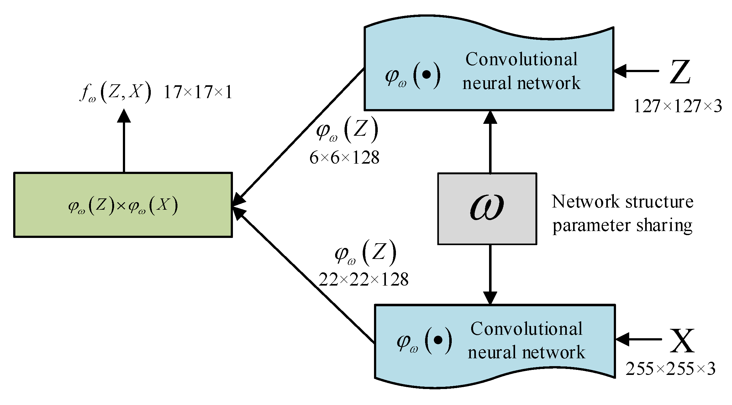
The tracking algorithm based on deep learning can be divided into two types—online fine-tuning algorithm and offline training algorithm. The running speed of an online fine-tuning algorithm is only a few frames per second, while in offline training, the running speed of the algorithm can reach 100 frames per second, and the accuracy of the two is almost the same [18,19]. Asthe demand of real-time tracking is 30 frames per second, the online tuning algorithm struggles to meet the requirements, so the research object is the deep learning tracking algorithm based on offline training. The deep learning type of offline training can be pre-trained for video data sets. After a long time of pre-training, the network model can become particularly robust. However, the most prominent difficult problem in long-term tracking, that is, the occlusion and disappearance of the target, will lead to tracking failure. Therefore, on the basis of SiamRPN, an attention mechanism is introduced to solve the problem of long-term tracking and make tracking more accurate. A twin network is composed of two convolutional neural subnetworks with the same structure and parameters, which is a special deep learning architecture of the monocular tracking algorithm [20]. The input of the network is a pair of images called model images and search images [21]. Offline learning involves obtaining the feature map of two images by forward-computing the subnet. Finally, the similarity measure of two images is calculated by the similarity measure function, which is substituted for the loss function, and the network parameters of a given label are adjusted by the back-propagation gradient. The form of the loss function is shown in Equation (1).

$$L\left(\mathsf{\omega }\left(Y,Z,X\right)\right)=\left(1-Y\right)L_{+}\left(f_{\mathsf{\omega }}\left(Z,X\right)\right)+Y{L}_{-}\left(f_{\mathsf{\omega }}\left(Z,X\right)\right)$$

(1)

In Equation (1), $Z$ is the model image, $X$ is the search image, and $Y$ is the truth marker of the image pair. $Y=0$. The corresponding loss function is $L_{+}$ for image pairs with the same target and $Y=1$ for image pairs with different targets and $L_{-}$ for the corresponding loss function. Figure 1 shows a typical construction of a twin network model.

As can be seen from Figure 1, the input, output and intermediate feature diagram dimensions of the study design (the feature diagram is $H\times W\times C$) are represented by the numbers on the diagram, with $AlexNet$ selected as ${\mathsf{\phi }}_{\mathsf{\omega }}\left(.\right)$, and $\star$ representing the inter-correlation operation. From Figure 1, Equation (2) can be derived as follows:

$$f_{\mathsf{\omega }}\left(Z,X\right)={\mathsf{\phi }}_{\mathsf{\omega }}\left(Z\right)\star {\mathsf{\phi }}_{\mathsf{\omega }}\left(X\right)$$

(2)

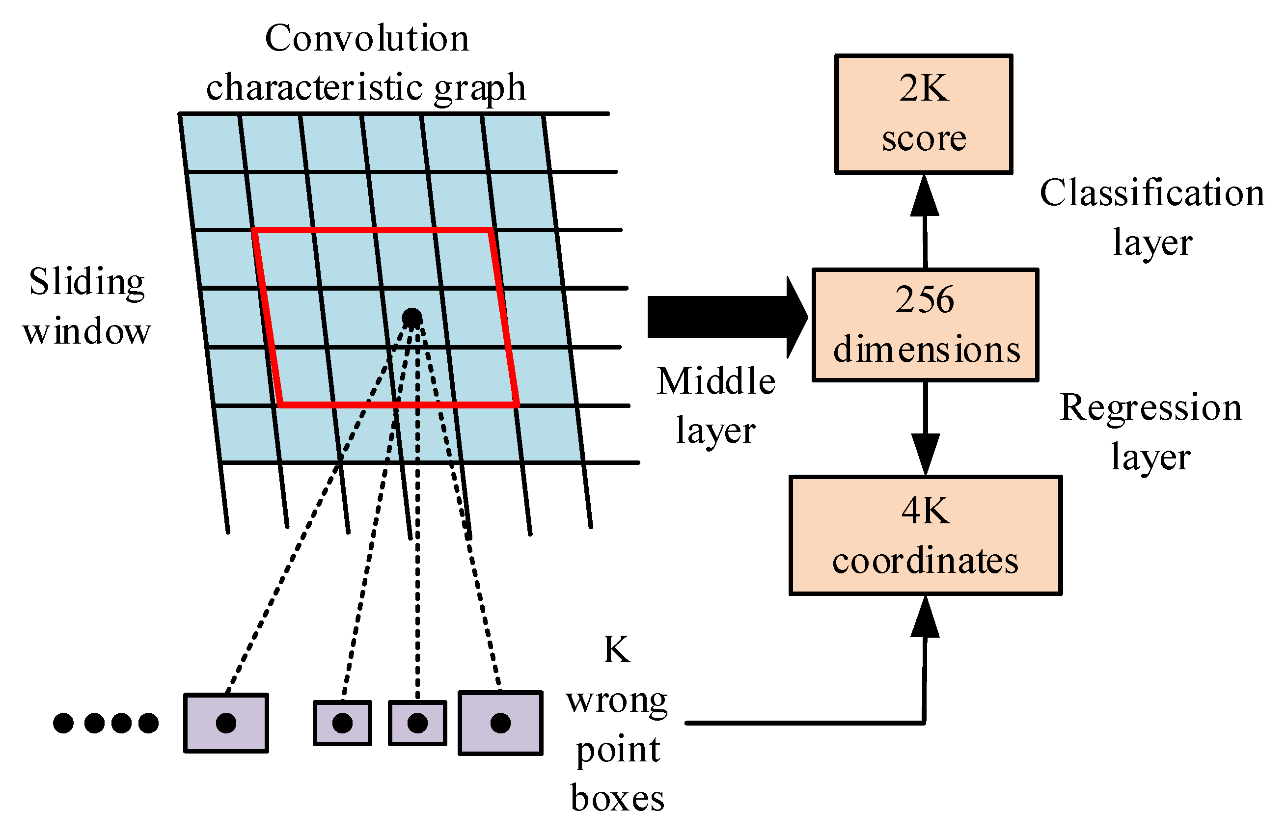
In Equation (2), ${\mathsf{\phi }}_{\mathsf{\omega }}\left(.\right)$ represents a sub-network that extracts the depth characteristics of an image, $f_{\mathsf{\omega }}\left(Z,X\right)$ represents the similarity of two depth features, and $\star$ represents the interrelated operations. When a dual network is employed for tracking, typically, the model image is selected from the first frame of the video representing the tracked objects and their locations, while the retrieved frames are selected from the subsequent video frames. Using Equation (2), the similarity index of the next frame to the previous frame can be derived and the position of the tracked object and the position of the tracked object within the next frame can thus be found for continuous tracking. The Region Proposal Network (RPN) is implemented using a convolutional neural network for the input of a picture and outputs a set of rectangular candidate regions with a score that indicates the probability of the location of the target in that region, the structure of which is shown in Figure 2.

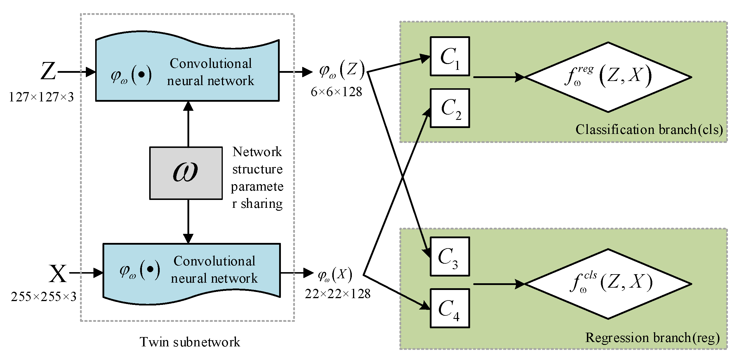
As can be seen in Figure 2, the output feature map of the convolutional layer, fed through a sliding window of size 3 × 3 in the RPN, produces a 256-dimensional feature output. These features are fully concatenated and fed into two layers, one predicting the probability of an object appearing in a candidate image and the other predicting the coordinates of the candidate image (X, Y, W, H). For each position in the sliding window, the RPN should predict k candidate fields, the classification layer should classify objects and backgrounds such that the output is 2k, and the regression layer should predict coordinates such that the output is 4k. To allow for parametric manipulation, the study introduces k anchor points corresponding to each candidate image. The introduction of the anchor points allows the calculation of the Intersection-over-Union (IoU) ratio between the anchor points and the calibration frame. If the IoU is above a certain threshold, the anchor is considered as a positive sample, if the IoU is below a certain threshold, the anchor is considered as a negative sample, so that the network model can know whether an object is present at that anchor. The twin region suggestion network (SiamRPN) is an improved version of the SiamFC structure with the addition of the RPN, so that its overall structure consists of a twin sub-network and a region suggestion sub-network, as shown in Figure 3.

As can be seen in Figure 3, the input to the network is also a pair of images and the deep feature extraction is also performed on this pair of images in a twin sub-network, but the difference is that the tracking task is treated as a single target recognition task due to the introduction of the region proposal sub-network. The proposed region sub-network is divided into a classification branch at the top and a regression branch at the bottom. The depth feature ${\mathsf{\phi }}_{\mathsf{\omega }}\left(Z\right)$ of the template image $Z$ is convolved on the convolutional layer $C_1$ in the classification branch to obtain $C_1{}^{{\mathsf{\phi }}_{\mathsf{\omega }}\left(Z\right)}$, and the number of channels becomes $2k\times 256$; ${\mathsf{\phi }}_{\mathsf{\omega }}\left(Z\right)$ is convolved on the regression branch of the convolutional layer $C_3$ to obtain $C_3{}^{{\mathsf{\phi }}_{\mathsf{\omega }}\left(Z\right)}$, and the number of channels becomes $4k\times 256$. After the second convolution of the search image $X$ on the two branches $C_2$ and $C_4$, the depth characteristics are obtained as ${\mathsf{\phi }}_{\mathsf{\omega }}\left(X\right)$$C_2{}^{{\mathsf{\phi }}_{\mathsf{\omega }}\left(Z\right)}$ and $C_4{}^{{\mathsf{\phi }}_{\mathsf{\omega }}\left(Z\right)}$, respectively, with the same number of channels. Then, by using the similarity measure function in each branch, the similarity on the classification branch $f_{\mathsf{\omega }}^{cls}\left(Z,X\right)$ can be obtained as shown in Equation (3).

$$f_{\mathsf{\omega }}^{cls}\left(Z,X\right)=C_1^{{\mathsf{\phi }}_{\mathsf{\omega }}\left(Z\right)}\star C_2^{{\mathsf{\phi }}_{\mathsf{\omega }}\left(X\right)}$$

(3)

The similarity in the regression branch $f_{\mathsf{\omega }}^{reg}\left(Z,X\right)$ is shown in Equation (4).

$$f_{\mathsf{\omega }}^{reg}\left(Z,X\right)=C_3^{{\mathsf{\phi }}_{\mathsf{\omega }}\left(Z\right)}\star C_4^{{\mathsf{\phi }}_{\mathsf{\omega }}\left(X\right)}$$

(4)

The essence of the twin region suggestion network is to learn the similarity between two images, and the introduction to RPN is to make full use of the image information on the object being tracked in the first frame of the video, to generate as many candidate frames as possible to match the images in subsequent frames, and to enable the network to handle multi-scale problems. The SiamRPN algorithm balances the requirements for accuracy and real-time performance in the tracking problem. It is designed for arbitrary short-term tracking tasks, but still has drawbacks when applied to long-term tracking systems for athletes.

3.2. A SingleTarget Long-Time Tracking Framework Based on Improved SiamRPN

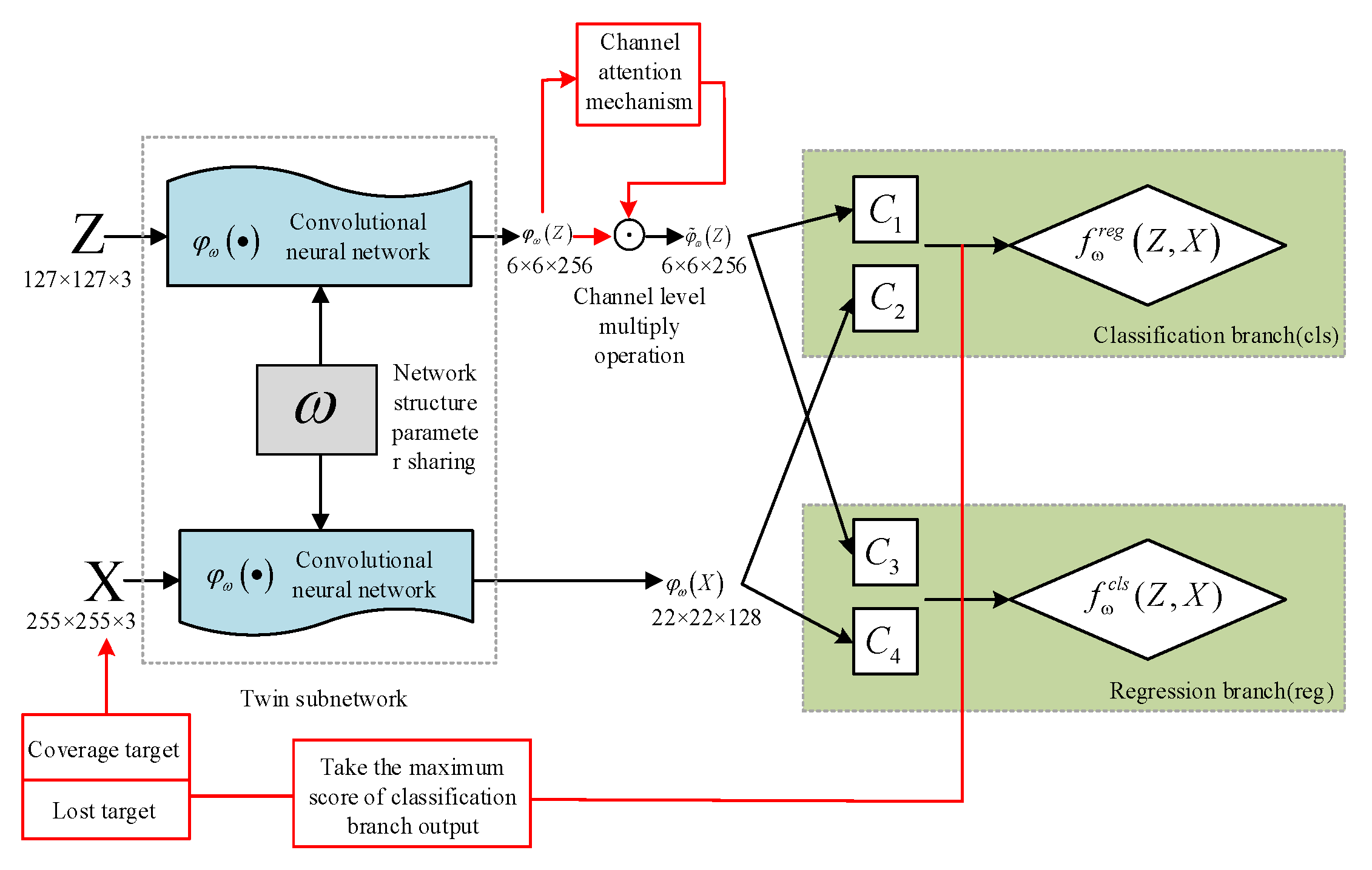
The feature channels of the convolution layer correspond to certain features of the object, and different feature channels contribute differently to the final similarity measure. Therefore, if the tracking target is set for an athlete, then the features of the athlete should be more important than the features of other objects. In contrast, SiamRPN does not set specific targets for athletes, and therefore, tracking for athletes is not ideal. In addition to this, the ultra-long range and complete occlusion of the target create additional problems for long-term tracking, as the search range of the SiamRPN algorithm does not cover the target in its entirety when it reappears, thus causing the target tracking to fail [22,23]. To address these issues, the study introduces a channel attention mechanism for the SiamRPN model branch, increasing the weight of important features and searches, and a local–global search strategy so that tracking can continue when the target leaves the field of view or reappears after complete occlusion, with the structure of the improved network shown in Figure 4.

As can be seen in Figure 4, the channel focus mechanism proposed in the study is only applicable on the model branch, i.e., the filtering process of the semantic attributes of the different feature channels of the model image extracted by the twin network. During the tracking process, the contribution of different channels will theoretically change when the target scale changes or occlusion occurs, but the different channels need to be given corresponding weights in order to accommodate the various target change during the tracking process. Furthermore, as the channel attention proposed in the study is learned in the offline stage and does not require online fine-tuning of parameters during tracking, but only forward computation, the introduction of channel attention in the model branch of the twin network will not have a significant impact on the overall network speed. The structure of channel attention is shown in Figure 5.

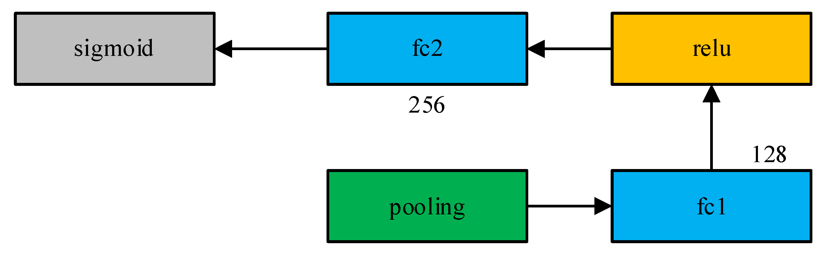
As can be seen from Figure 5, the channel attention structure consists of a pooling layer, two fully connected layers, a ReLU activation function, and a sigmoid activation function. The pooling layer is a Global Average Pooling (GAP) layer, which uses a sampling area of 6 × 6 with the same height and width as φ_ω (Z). Assuming a sampling area size of $f\times f$ and a sliding step of $s$, Equation (5) calculates the size of the feature map for each channel after the global average pooling layer.

$$\left\{\begin{array}{l}{H}_{out}=⌊\frac{H_{in}-f}{s}+1⌋\\ W_{out}=⌊\frac{W_{in}-f}{s}+1⌋\end{array}\right.$$

(5)

The size of the feature map for each channel is obtained from Equation (5) as 1 × 1. The channel note eventually learns a one-dimensional weight distribution, but since its input is a three-dimensional 6 × 6 × 256 matrix, the global intermediate layer serves to reduce the dimensionality equally by reducing the three-dimensional 6 × 6 × 256 matrix to a one-dimensional 256 vector.

As this fully connected layer fc1 has 128 neurons, the output of this layer is a vector of length 128 whose task is to combine the features extracted from the previous layer and the output of the fully connected layer is activated by the activation function ReLU. Finally, the fully connected layer fc2 with a sigmoid activation function of 256 neurons ensures that the number of features filtered through the attention channel is the same as the original number of features, so that the final output of the attention channel is a vector of weight distribution of length 256. The twin network template branch outputs a feature map of ${\mathsf{\phi }}_{\mathsf{\omega }}\left(Z\right)$, which is assumed to have a feature channel set of ${\mathsf{\phi }}_{\mathsf{\omega }}\left(Z\right)=\left[b_1,b_2,\dots ,b_n\right],b_i\in R^{H\times W},i=1,2,\dots ,n$, where $n$ is the number of channels. By assigning the corresponding weights to ${\mathsf{\phi }}_{\mathsf{\omega }}\left(Z\right)$ through the channel-level operation shown in Equation (6), the final result is ${\tilde{\mathsf{\phi }}}_{\mathsf{\omega }}\left(Z\right)$, whose set of feature channels is $\stackrel{\sim }{{\mathsf{\phi }}_{\mathsf{\omega }}\left(Z\right)}=\left[\stackrel{\sim }{b_1},\widetilde{b_2},\dots ,\widetilde{b_n}\right],\widetilde{b_l}\in R^{H\times W},i=1,2,\dots ,n$.

$$\left\{\begin{array}{l}\widetilde{b_l}={\mathsf{\beta }}_i·b_i,i=1,2,\dots ,n\\ \stackrel{\sim }{{\mathsf{\phi }}_{\mathsf{\omega }}\left(Z\right)}=\mathsf{\beta }\odot {\mathsf{\phi }}_{\mathsf{\omega }}\left(Z\right)\end{array}\right.$$

(6)

In Equation (6), $\mathsf{\beta }=\left[{\mathsf{\beta }}_1,{\mathsf{\beta }}_2,\dots ,{\mathsf{\beta }}_n\right],{\mathsf{\beta }}_i\in R,i=1,2,\dots$,$n$ represents the attention of ${\mathsf{\phi }}_{\mathsf{\omega }}\left(Z\right)$ through the channel $C_{\mathsf{\beta }}$ weights for subsequent outputs; $\odot$ is a channel-level multiplication operation to study the number of channels output from the twin network template branches $n=256$. Long-term monitoring tasks, in addition to considering the difficulties of short-term monitoring that must be overcome, must also take into account the additional challenges that over-distance field of view ranges and complete target occlusion may pose to long-term monitoring. Therefore, the study proposes a simple and effective method based on SiamRPN for switching from localtoglobal search areas. The classification branch of the SiamRPN region suggestion sub-network is responsible for predicting the probability of the presence of an object in a candidate image, while the feedback branch is responsible for predicting the coordinates of the candidate image. The combination is a set of candidate regions with scores, with the highest score Smax being used to determine the beginning and end of the tracking error. With a threshold t_begin for entering a fault situation and a threshold t_end for exiting a fault situation, t_end > t_begin. If Smax < t_begin, then a fault situation is indicated and the initial search area of size 255 × 255 fails to detect the re-emerging object, so a local-whole strategy must be used to extend the search area. If Smax is no longer equal to any of the sizes Smax < t_begin, then iterative growth is no longer required. Once Smax > t_begin is reached, the search area is covered again and reverts to its original size of 255 × 255 and the size of the search area is used for further tracking. The thresholds set for the study were t_begin = 0.8 and t_end = 0.95. The similarity on the classification branch $f_{\mathsf{\omega }}^{cls}\left(Z,X\right)$ can be obtained from Figure 4 as shown in Equation (7).

$$f_{\mathsf{\omega }}^{cls}\left(Z,X\right)=C_1^{{\tilde{\mathsf{\phi }}}_{\mathsf{\omega }}\left(Z\right)}\ast C_2{}^{{\mathsf{\phi }}_{\mathsf{\omega }}\left(X\right)}$$

(7)

In Equation (7), the convolution of ${\tilde{\mathsf{\phi }}}_{\mathsf{\omega }}\left(Z\right)$ with the convolution layer $C_1$ in the classification branch is performed to obtain $C_1^{{\tilde{\mathsf{\phi }}}_{\mathsf{\omega }}\left(Z\right)}$ with the number of feature channels $2k\times 256$, and ${\mathsf{\phi }}_{\mathsf{\omega }}\left(X\right)$ is convolved by the classification branch $C_2$ to obtain $C_2{}^{{\mathsf{\phi }}_{\mathsf{\omega }}\left(X\right)}$. The similarity on the regression branch $f_{\mathsf{\omega }}^{reg}\left(Z,X\right)$ is shown in Equation (8)

$$f_{\mathsf{\omega }}^{reg}\left(Z,X\right)=C_3^{\stackrel{\sim }{{\mathsf{\phi }}_{\mathsf{\omega }}\left(Z\right)}}\star C_4^{{\mathsf{\phi }}_{\mathsf{\omega }}\left(X\right)}$$

(8)

In Equation (8), the convolution of ${\tilde{\mathsf{\phi }}}_{\mathsf{\omega }}\left(Z\right)$ with the convolution layer $C_3$ in the regression branch is performed to obtain $C_3^{{\tilde{\mathsf{\phi }}}_{\mathsf{\omega }}\left(Z\right)}$ with the number of feature channels $4k\times 256$, and ${\mathsf{\phi }}_{\mathsf{\omega }}\left(X\right)$ is convolved by the regression branch $C_4$ to obtain $C_4{}^{{\mathsf{\phi }}_{\mathsf{\omega }}\left(X\right)}$. From Equation (6), the similarity $f_{\mathsf{\omega }}^{cls}\left(Z,X\right)$ on the classification branch can be refined to Equation (9)

$$f_{\mathsf{\omega }}^{cls}\left(Z,X\right)=C_1^{\mathsf{\beta }\odot {\mathsf{\phi }}_{\mathsf{\omega }}\left(Z\right)}\star C_2{}^{{\mathsf{\phi }}_{\mathsf{\omega }}\left(X\right)}$$

(9)

We refine the similarity on the regression branch $f_{\mathsf{\omega }}^{reg}\left(Z,X\right)$ to Equation (10).

$$f_{\mathsf{\omega }}^{reg}\left(Z,X\right)=C_3^{\mathsf{\beta }\odot {\mathsf{\phi }}_{\mathsf{\omega }}\left(Z\right)}\star C_4^{{\mathsf{\phi }}_{\mathsf{\omega }}\left(X\right)}$$

(10)

For offline training, the study used the same loss function as SiamRPN, with cross-entropy loss for the classification branch and smooth $L_1$ loss for the regression branch. Assuming that $A_x,A_y,A_W,A_h$ represents the coordinates of the anchor point, $y_A$ represents the probability of the anchor point predicting the presence of the target, $T_x,T_y,T_w,T_h$ represents the coordinates of the calibration frame, and $y_T$ represents the probability of the presence of the true target, the regularized distance $d\left[0\right],d\left[1\right],d\left[2\right],d\left[3\right]$ is as shown in Equation (11).

$$\left\{\begin{array}{l}d\left[0\right]=\frac{T_x-A_x}{A_W}\\ d\left[1\right]=\frac{T_y-A_y}{A_h}\\ d\left[2\right]=\ln \frac{T_w}{A_w}\\ d\left[3\right]=\ln \frac{T_h}{A_h}\end{array}\right.$$

(11)

The expression for the loss of smooth $L_1$ is shown in Equation (12).

$$smoot{h}_{L_1}\left(x\right)=\left\{\begin{array}{l}0.5x^2,if\left|x\right|<1\\ \left|x\right|-0.5,otherwise\end{array}\right.$$

(12)

Substituting Equation (11) into Equation (12) yields the loss of the regression branch, as shown in Equation (13).

$$L_{reg}={\displaystyle \sum _{i=0}^{3}smoot{h}_{L_1}\left(d\left[i\right]\right)}$$

(13)

The loss of the classification branch is shown in Equation (14).

$$L_{cls}=C\left(y_A,y_T\right)=-\frac{1}{n}{\displaystyle \sum y_T\ln y_A+\left(1-y_T\right)\ln \left(1-y_A\right)}$$

(14)

The final loss function obtained for the whole is shown in Equation (15).

$$loss=L_{reg}+L_{cls}$$

(15)

4. Performance Testing of the Target Long-Time Tracking Algorithm Model

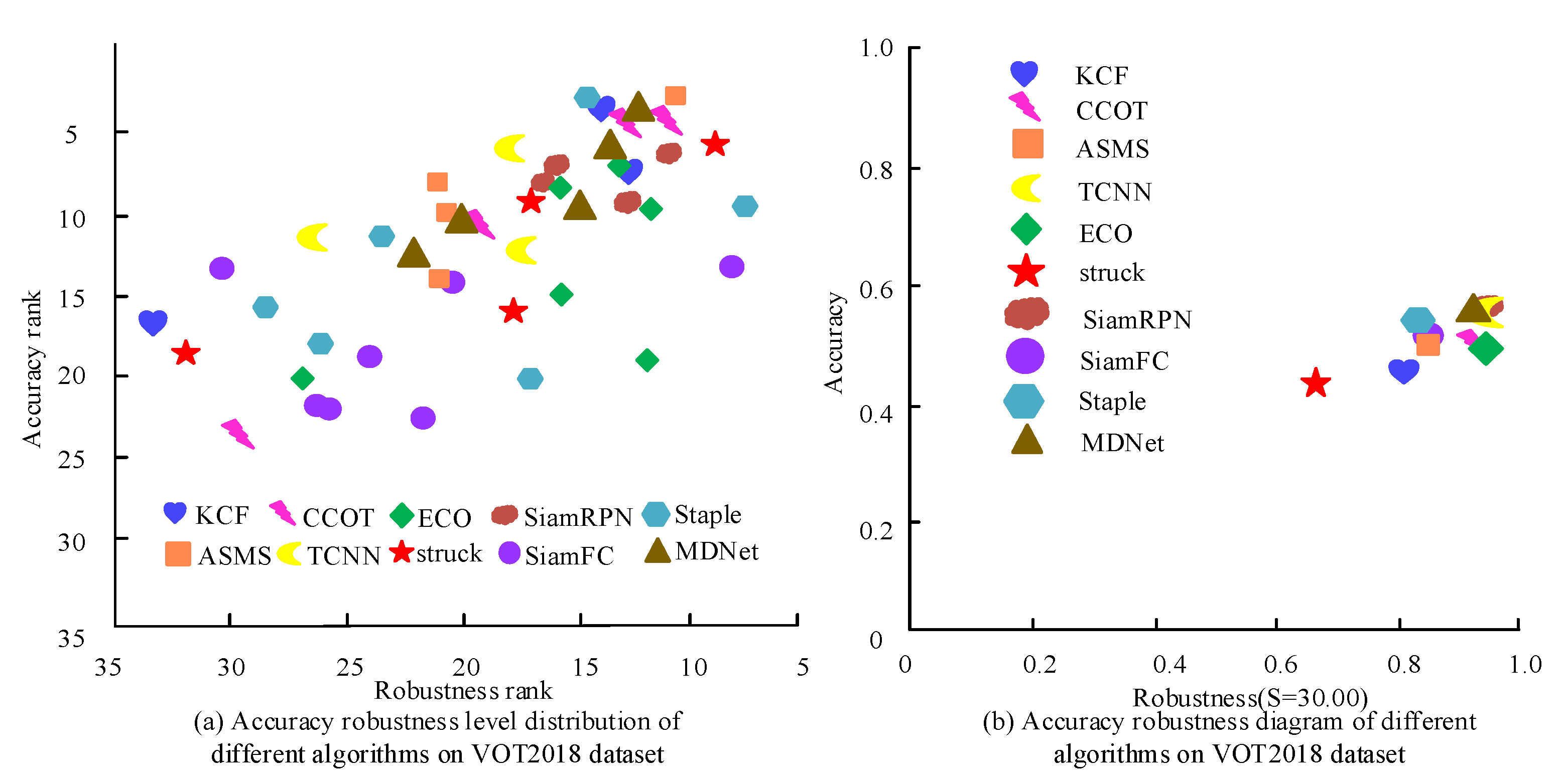
In order to implement an athlete tracking model, the tracking algorithm used must meet the criteria of excellence and speed. The performance of the tracking algorithms was measured experimentally using Accuracy–Robustness (AR) plots and Frame Rate (Frames Per Second, FPS) was chosen as a measure of how fast the tracking algorithms worked. In order to better compare the performance of SiamFC and SiamRPN, benchmark algorithms such as KCF, CCOT, ECO, Staple, MDNet, struck, TCNN, and ASMS were introduced in the experiments for comparison. VOT2018 containing 60 selected video sequences was selected as the test dataset. In addition, the VOT-2018 LTB35 dataset was selected as the validation set, including 35 videos of people in specific situations involving cars, motorcycles, or bicycle lights. The AR plots obtained from the experiments are shown in Figure 6.

The closer the tracking algorithm is to the top right, the higher its accuracy and stability. As can be seen from Figure 6, the TCNN, SiamRPN, and MDNet algorithms perform best, but TCNN and MDNet are deep learning tracking algorithms that rely on online fine-tuning and require constant adjustment of model parameters in order to adapt to various changes in the tracking process. As a result, TCNN and MDNet are time-consuming and run very slowly. The specific performance values of each algorithm are shown in

Table 2. Robustness, accuracy and FPS comparison results of different algorithm tests.

Tracking Algorithm	Robustness	Accuracy	FPS
ASMS	35	0.476	132
TCNN	15	0.534	1
struck	80	0.405	15
Staple	42	0.522	45
MDNet	23	0.531	1
ECO	16	0.463	3
KCF	50	0.440	63
CCOT	22	0.475	0.3
SiamFC	37	0.502	88
SiamRPN	18	0.548	158

.

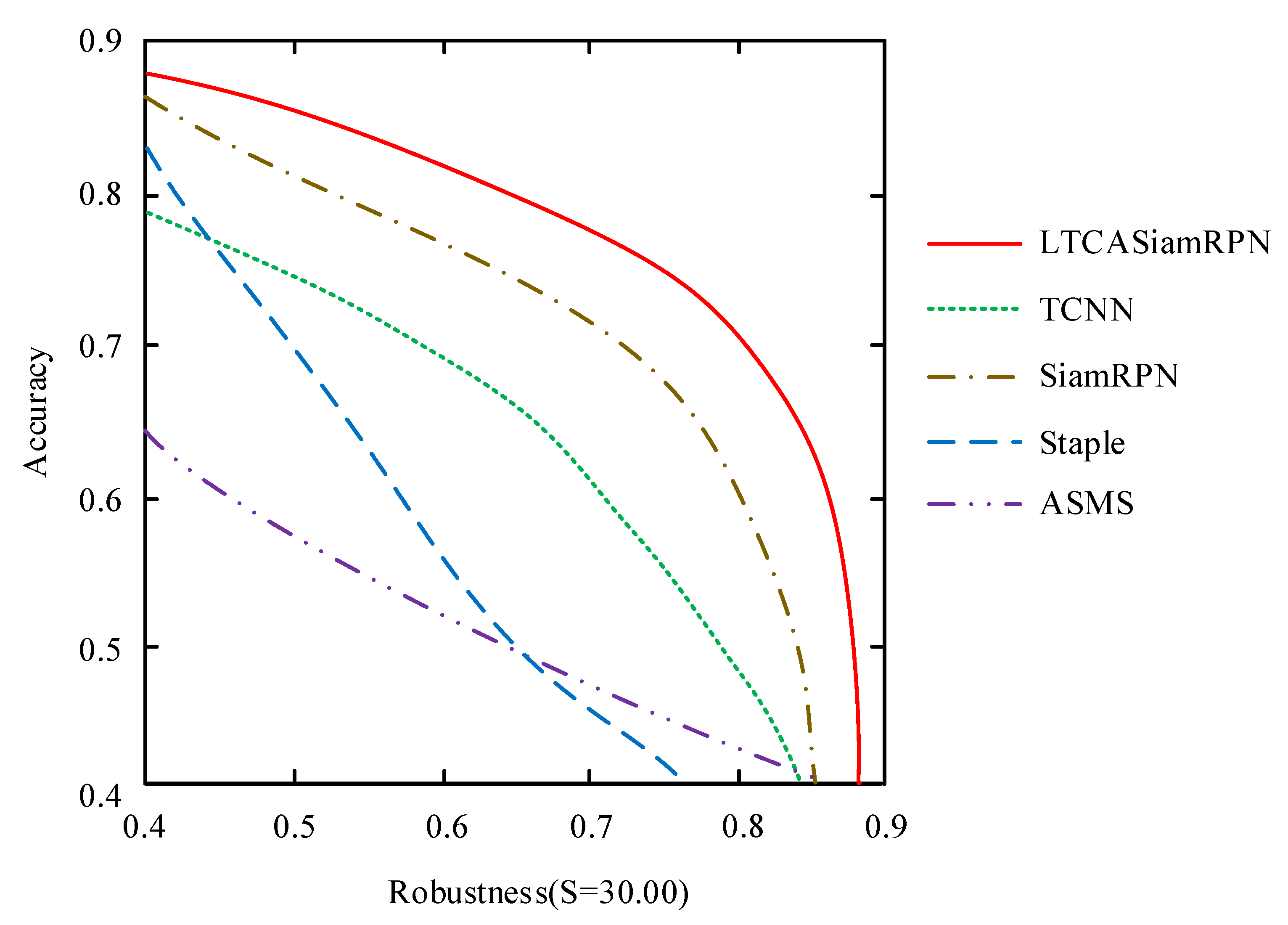
It can be seen from Table 2 that although the accuracy of SiamFC is only average, its operation speed is very fast, and FPS can reach 88. Sinceit does not need to adjust the model parameters online, SiamFC has greaterpractical application value. In terms of tracking, deep learning gradually tends to twin networks. Using twin networks, the identification problem can be transformed into a similarity measurement problem. This method can not only ensure accuracy, but it can also ensure operation speed. Unlike other tracking algorithms, the higher the accuracy, the slower the operation. At the same time, SiamFC also has the problem of poor robustness. By comparing SiamRPN with other tracking algorithms, it is found that SiamRPN has better accuracy and robustness, with the highest FPS value of 158, which is far beyond the real-time requirements of motion trajectory. After adding RPN to SiamFC, the recognition accuracy of SiamRPN is improved by 9.2%. The algorithm for comprehensive optimization is named improved SiamRPN, which is compared with five benchmark algorithms such as TCNN. The accuracy and robustness of the algorithm obtained from the experiment are shown in Figure 7.

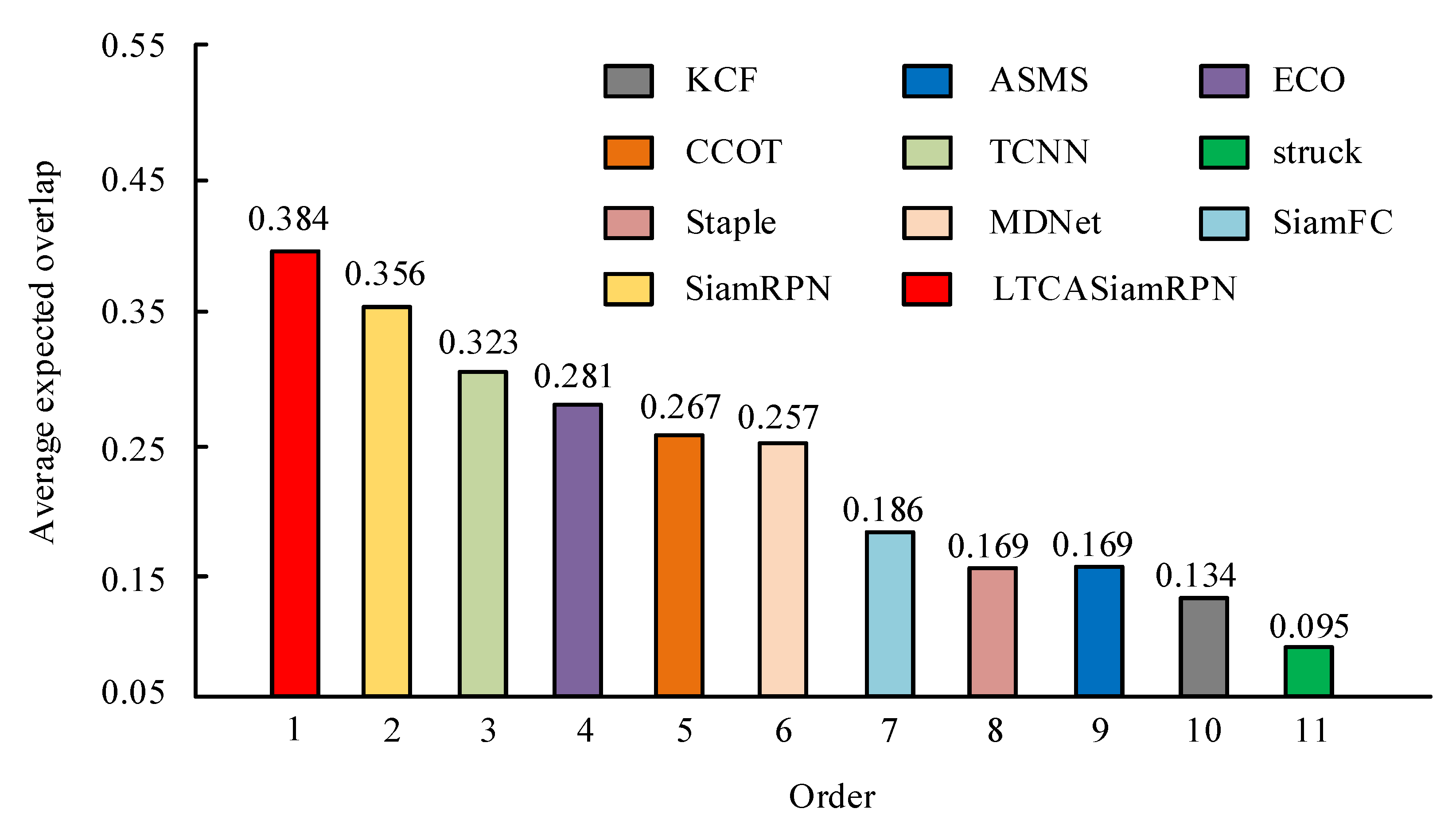
The closer the tracking algorithm is to the upper right, the higher the accuracy and stability of the algorithm. It can be seen from Figure 7 that the accuracy robustness of improved SiamRPN is the best compared with other benchmark algorithms. Aiming at the problem that the AR sorting method cannot make good use of the accuracy and robustness of the original data, we study the use of expected average overlap (EAO) to detect the performance of the algorithm, as shown in Figure 8, which shows the comparison of EAO point graphs of different algorithms. EAO point diagrams of improved SiamRPN, SiamRPN, and TCNN algorithm models ranked first, second, and third, respectively.

The specific test data in

Table 3. Comparison of Test Metrics for Different Algorithms.

Tracking Algorithm	Robustness	Accuracy	FPS	EAO
ASMS	35	0.476	132	0.169
TCNN	15	0.534	1	0.323
struck	80	0.405	15	0.095
Staple	42	0.522	45	0.169
MDNet	23	0.531	1	0.257
ECO	16	0.463	3	0.281
KCF	50	0.440	63	0.134
CCOT	22	0.475	0.3	0.267
SiamFC	37	0.502	88	0.186
SiamRPN	18	0.548	158	0.356
improved SiamRPN	17	0.578	118	0.384

show that compared with other algorithms, the accuracy of improved SiamRPN is 8.2% higher than TCNN and 5.5% higher than SiamRPN; The robustness is equivalent to the performance of SiamRPN and TCNN; EAO is higher than SiamRPN by 2.8 percentage points. FPS ranks third. Although it lags behind theSiamRPN and ASMS algorithms, its 118 rate still far exceeds the real-time requirements (the real-time standard is 30 fps).

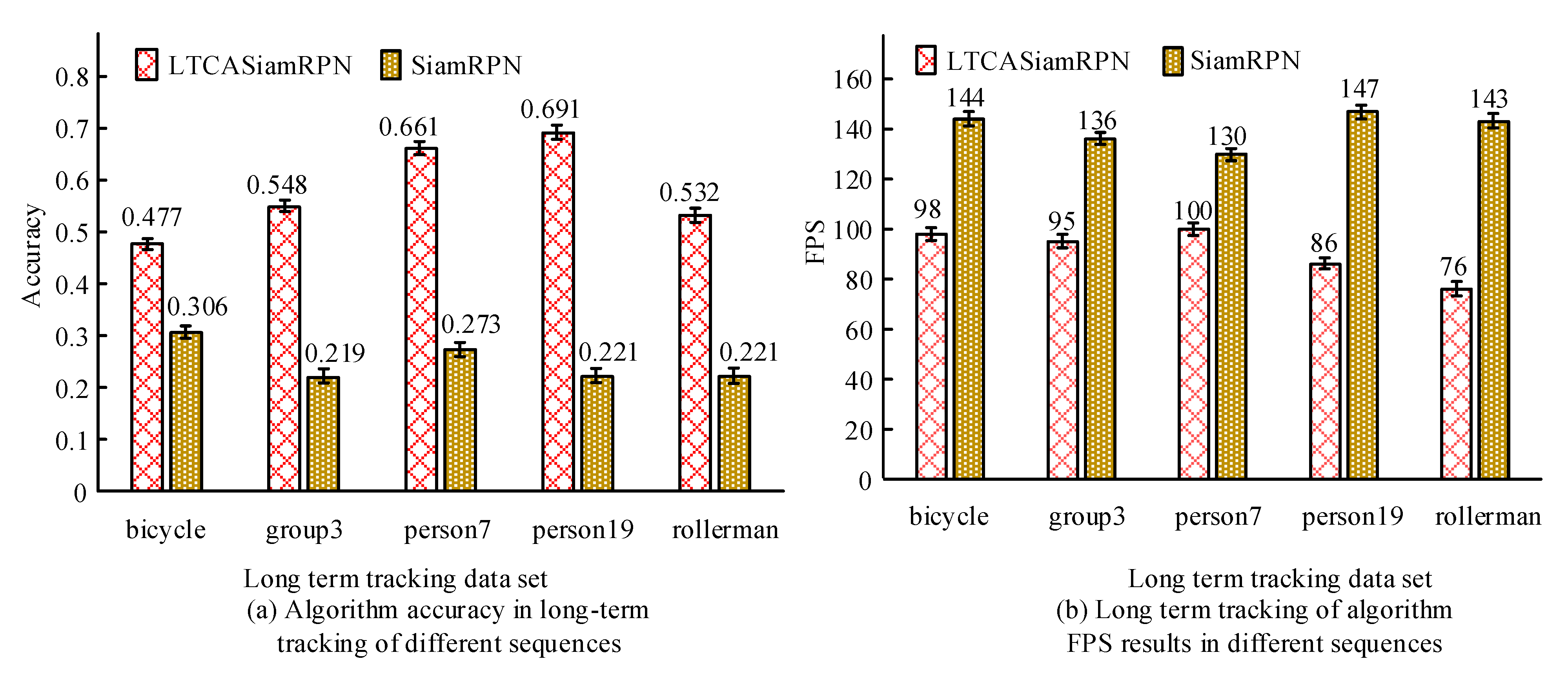
The tracking work in the vot2018 long-term tracking data set is mainly manifested in the rapid movement of the target, the movement of the camera and the continuous turnover and change of the line of sight, the frequent change of the target scale, and the easy occlusion of the target. In order to test the performance of the improved SiamRPN algorithm on the vot2018 long-term tracking data set, five challenging sequences were selected as test samples, and the performance was compared with the original SiamRPN algorithm. In the experiment, the tracking target of the algorithm was human, which was consistent with the object to be tracked by the research.

We comparethe accuracy of improved SiamRPN algorithm and SiamRPN algorithm with FPs to test the performance of improved SiamRPN algorithm in long-term tracking. The experimental results are shown in Figure 9. It can be seen from Figure 9 that the operation speed of the improved SiamRPN algorithm on five long-term tracking sequences is 49 MIPS slower than that of the original SiamRPN algorithm, but its accuracy is significantly higher than that of the original SiamRPN algorithm. This shows that when the tracking target disappears and reappears again, the local global search strategy has a good solution. The five sequences selected in the study contain a large number of target disappearances and other problems. The improved SiamRPN algorithm has a good response mechanism, which shows that the improved algorithm has excellent comprehensive performance in the long-term tracking data set.

5. Conclusions

A high-level sports event often depends on the tactical arrangement of coaches. Whether it is possible to accurately obtain the athletes’ sport status plays a key role in the tactical deployment of coaches. Thanks to the continuous development and improvement of deep convolution neural network, the application of deep learning in the field of vision is also deepening. At present, SiamFC and SiamRPN are widely used in offline training. As an extension of the SiamFC algorithm, SiamRPN has better accuracy and robustness, and FPS value far exceeds the demand of real-time performance. However, SiamRPN is only suitable for short-term tracking of a single target, not for long-term tracking of athletes. Aiming at resolving the difficulties of SiamRPN tracking technology in long-term tracking, an improved scheme based on the SiamRPN algorithm is proposed, that is, a channel attention mechanism and a local global search strategy are introduced into SiamRPN algorithm. The performance of the improved SiamRPN algorithm is tested on the vot2018 data set. The research results show that the improved SiamRPN algorithm has better accuracy robustness performance and higher prediction average overlap rate than the original SiamRPN algorithm. In the long-term target tracking task, the improved SiamRPN algorithm is slightly slower than SiamRPN algorithm, but it maintains a higher accuracy. This shows that the improved algorithm improves the tracking ability of the key features of the target, and it can repeat the coverage and continue to track when the target reappears. A method based on the twin structure is proposed, which transforms the tracking problem into the similarity measurement problem. This method has been proved to be effective in experiments. However, in follow-up work, if the historical information can be imported into the tracking process, the identification effect of tracking problems can be further improved.

References

- Dergaa, I.; Saad, H.B.; Souissi, A.; Musa, S.; Abdulmalik, M.A.; Chamari, K. Olympic Games in COVID-19 times: Lessons learned with special focus on the upcoming FIFA World Cup Qatar 2022. Br. J. Sport. Med. 2022, 56, 654–656. [Google Scholar] [CrossRef] [PubMed]
- Bianco, S.; Napoletano, P.; Raimondi, A.; Rima, M. U-WeAr: User Recognition on Wearable Devices through Arm Gesture. IEEE Trans. Hum. Mach. Syst. 2022, 52, 713–724. [Google Scholar] [CrossRef]
- Zhou, X.; Wang, P.; Chan, S.; Fang, K.; Fang, J. Densely connected Siamese network visual tracking. Ind. Robot. Int. J. Robot. Res. Appl. 2021, 48, 680–687. [Google Scholar]
- Xing, R.; Zhang, W.; Shu, L.; Zhang, B. An Autonomous Moving Target Tracking System for Rotor UAV 2021 International Conference on Robotics and Control Engineering; ACM: New York, NY, USA, 2021; pp. 48–53. [Google Scholar]
- Wu, C.; Fu, T.; Wang, Y.; Lin, Y.; Wang, Y.; Ai, D.; Fan, J.; Song, H.; Yang, J. Fusion Siamese network with drift correction for target tracking in ultrasound sequences. Phys. Med. Biol. 2022, 67, 045018. [Google Scholar] [CrossRef] [PubMed]
- Reddy, B.M.; Rahman, M. Novel Segmentation Technique for Target Tracking in Synthetic Aperture Radars. Int. J. Comput. Intell. Theory Pract. 2021, 16, 113–119. [Google Scholar]
- Kent, J.S.; Wamsley, C.C.; Flateau, D.; Ferguson, A. Unsupervised learning for target tracking and background subtraction in satellite imagery. SPIE 2021, 11746, 2021–2030. [Google Scholar]
- Koteswara, R.S.; Omkar Lakshmi Jagan, B.; Kavitha, L.M. Underwater target tracking in three-dimensional environment using intelligent sensor technique. Int. J. Pervasive Comput. Commun. 2022, 18, 319–334. [Google Scholar]
- Jang, J.; Lee, C.; Kim, J. Ambiguity Resolution Between Constant Velocity and Coordinated Turn Models for Multimodel Target Tracking. IEEE Sens. Lett. 2022, 6, 1–4. [Google Scholar] [CrossRef]
- Farahmand, S.; Fernandez, A.I.; Ahmed, F.S.; Rimm, D.L.; Chuang, J.H.; Reisenbichler, E.; Zarringhalam, K. Deep learning trained on hematoxylin and eosin tumor region of Interest predicts HER2 status and trastuzumab treatment response in HER2+ breast cancer. Mod. Pathol. 2022, 35, 44–51. [Google Scholar] [CrossRef]
- Sato, H.; Igarashi, H. Deep learning-based surrogate model for fast multi-material topology optimization of IPM motor. COMPEL Int. J. Comput. Math. Electr. Electron. Eng. 2022, 41, 900–914. [Google Scholar] [CrossRef]
- Abdel-Basset, M.; Hawash, H.; Chakrabortty, R.K.; Ryan, M.; Elhoseny, M.; Song, H. ST-DeepHAR: Deep Learning Model for Human Activity Recognition in IoHT Applications. IEEE Internet Things J. 2021, 8, 4969–4979. [Google Scholar] [CrossRef]
- Kuutti, S.; Bowden, R.; Jin, Y.; Barber, P.; Fallah, S. A Survey of Deep Learning Applications to Autonomous Vehicle Control. IEEE Trans. Intell. Transp. Syst. 2021, 22, 712–733. [Google Scholar] [CrossRef]
- Duan, S.; Xiang, J.; Yu, X. A model-driven robust deep learning wireless transceiver. IET Commun. 2021, 15, 2252–2258. [Google Scholar] [CrossRef]
- Wang, Z.; Wang, J.; Fan, R. An underwater single target tracking method using SiamRPN++ based on inverted residual bottleneck block. IEEE Access 2021, 99, 25148–25157. [Google Scholar] [CrossRef]
- An, N.; Yan, W.Q. Multitarget tracking using Siamese neural networks. ACM Trans. Multimed. Comput. Commun. Appl. 2021, 17, 1–16. [Google Scholar] [CrossRef]
- Subrahmanyam, K.; Kavitha, L.M.; Rao, S.K. Shifted Rayleigh filter: A novel estimation filtering algorithm for pervasive underwater passive target tracking for computation in 3D by bearing and elevation measurements. Int. J. Pervasive Comput. Commun. 2022, 18, 272–287. [Google Scholar]
- Ramkumar, M.; Yadav, R.; Yadav, S. Deep Learning Approach for Radical Sound Valuation of Fetal Weight. ECS Trans. 2022, 107, 2735–2747. [Google Scholar]
- Han, Y.; Lam, J.C.; Li, V.O.; Zhang, Q. A Domain-Specific Bayesian Deep-Learning Approach for Air Pollution Forecast. IEEE Trans. Big Data 2022, 8, 1034–1046. [Google Scholar] [CrossRef]
- Delande, E.; Houssineau, J.; Franco, J.; Frueh, C.; Clark, D.; Jah, M. A new multi-target tracking algorithm for a large number of orbiting objects. Adv. Space Res. 2019, 64, 645–667. [Google Scholar] [CrossRef]
- Yu, X.; Jin, G.; Li, J. Target Tracking Algorithm for System with Gaussian/Non-Gaussian Multiplicative Noise. IEEE Trans. Veh. Technol. 2019, 69, 90–100. [Google Scholar] [CrossRef]
- Ankel, V.; Shribak, D.; Chen, W.Y.; Heifetz, A. Classification of computed thermal tomography images with deep learning convolutional neural network. J. Appl. Phys. 2022, 131, 244901. [Google Scholar] [CrossRef]
- Alshra’a, A.S.; Farhat, A.; Seitz, J. Deep Learning Algorithms for Detecting Denial of Service Attacks in Software-Defined Networks. Procedia Comput. Sci. 2021, 191, 254–263. [Google Scholar] [CrossRef]
Figure 1.
Twinning Network Structure Diagram.
Figure 2.
Regional Proposal Network Structure Map.
Figure 3.
Map of the Proposed Network Structure for Twin Regions.
Figure 4.
Diagram of the Improved SiamRPN Network Structure.
Figure 5.
Channel Attention Structure.
Figure 6.
Horizontal Distribution and Results of Accuracy Robustness of Different Algorithms on VOT2018 Dataset.
Figure 7.
Comparison of Accuracy–Robustness Experimental Results of Different Algorithms.
Figure 8.
EAO Point Diagram for Different Algorithms.
Figure 9.
Accuracy of different tracking algorithms and FPS comparison results.