

Simulation of Multi-Phase Flow in Autoclaves Using a Coupled CFD-DPM Approach
1
Faculty of Metallurgical and Energy Engineering, Kunming University of Science and Technology, Kunming 650093, China
2
State Key Laboratory of Complex Nonferrous Metal Resources Clean Utilization, Kunming University of Science and Technology, Kunming 650093, China
3
Metallurgical and Environmental Protection Department, Kunming Metallurgical Research Institute Co., Ltd., Kunming 650093, China
*
Author to whom correspondence should be addressed.
Processes 2023, 11(3), 890; https://doi.org/10.3390/pr11030890
Submission received: 21 February 2023
/
Revised: 12 March 2023
/
Accepted: 13 March 2023
/
Published: 15 March 2023
(This article belongs to the Special Issue Multiphase Mass Transfer and Phase Equilibrium in Chemical Processes)
Abstract
:In this work, a numerical simulation study on the mixing characteristics of multiphase flow in an autoclave was carried out using CFD technology. The Eulerian–Eulerian model and discrete phase model (DPM) were employed to investigate the solid holdup, critical suspension speed, nonuniformity of solid suspension, gas holdup distribution, bubble tracks, and residence time during stirring leaching in the autoclave. Experiments validate the accuracy of the numerical model, and the experimental values correspond well with the simulation results. The numerical simulation results show that the solid–liquid mixing is mainly affected by the axial flow, the best agitation speed is 400 rpm, and increasing the speed further cannot make the mixture more homogenous and buildup occurred above the autoclave. The calculated critical suspension speed is 406 rpm, which is slightly lower than that obtained from the empirical formula. The gas phase is mainly concentrated in the vortex area above the blade. When the gas phase is in a completely dispersed state (N = 300 rpm), the average residence time of the bubbles is 5.66 s.
1. Introduction
The autoclave is a pressurized stirred tank reactor that is widely used in the metal extraction processes of aluminum, zinc, lead, nickel, and complex refractory minerals in pressurized hydrometallurgy. In the pressure leaching process of metal, the gas used is generally oxygen. Taking the oxygen pressure leaching of zinc concentrate as an example, the way that oxygen participates in the leaching reaction is to dissolve in the leaching solution, so the leaching reaction is still a solid–liquid reaction process in nature [1]. Thus, the solid–liquid mixing effect in the autoclave has a great influence on the leaching reaction. Additionally, the solubility of oxygen in the leaching system is another crucial factor affecting the leaching reaction. According to the two-film theory of Lewis and Whitman [2], the volumetric mass transfer coefficient kLa can be used to quantify the gas–liquid mass transfer process. Among them, “kL” is the liquid mass transfer coefficient, which is mainly affected by the density and viscosity of the liquid medium and the gas–liquid affinity. Therefore, most of the current research on enhancing oxygen mass transfer focuses on increasing the gas–liquid interface area “a” which is easier to achieve [3,4,5,6]. However, limited by the aggressive and airtight conditions in the autoclave, it is difficult to quantitatively describe the multiphase mixing effect of solid–liquid or gas–liquid in the autoclave [7,8]. With the development of computer technology, the numerical simulation technology based on computational fluid dynamics (CFD) has been quite mature so far [9,10,11,12]. Computer numerical simulation is the primary method for expanding the reactor design and studying the characteristics of the flow field. It can obtain the characteristic parameters and information of the flow field that are difficult to obtain by traditional experimental methods.
Simulation research of the multiphase flow field in stirred tank reactors conducted by specialists and academics focuses primarily on the investigation of flow field characteristics and multiphase mixing characteristics. Ramírez-Torres et al. [13] performed an analysis of the computational hydrodynamic continuous stirred-tank behavior. The findings indicate that the optimal impeller configuration can reduce energy use by up to 9%. Gu et al. [14] used a CFD-PBM coupled model to study the hydrodynamic characteristics of the stirred tank. It was discovered that a self-similarity impeller can improve the uniformity of gas holdup distribution and facilitate the gas dispersion process. Cheng et al. [15] conducted a simulation study on the macroscopic mixing characteristics of gas–liquid–liquid in a turbo-propeller stirred tank by using the Euler model based on CFD software. The reliability of the model is verified by the experimental data of immiscible liquid–liquid mixing. Using the tracer, the mixing times and flow traces of the experiment are compared with the simulation results, and the findings demonstrate that the Reynolds stress model can accurately predict the flow field and mixing time. In order to calculate the local velocities, local concentrations, and concentration gradients inside the adsorber, García-Hernández et al. [16] carried out a 3D numerical simulation of the adsorption process. Several kinetic and transport characteristics were recorded while varying the stirring rate (30–200 rpm) and the initial pyridine concentration (99–487 mg/L). Fan et al. [17] studied the effect of adding baffles on the structure of the circulating flow in the stirring tank. The results show that the baffled agitated tank shows a larger overall circulation capacity for flow rates of different liquid levels, and the root mean square of the axial and radial pulsation velocities is stronger than that of the unbaffled tank. The addition of baffles enhances the overall fluctuation. Overall, the majority of simulation studies of multiphase flow concentrate on the mixing characteristics and optimization of the impeller or tank construction parameters. However, what is neglected by the majority of research is that the residence time of the bubbles is also critical as it relates to the mass transfer process.
On the basis of CFD theory, the finite volume approach is utilized to create a multiphase flow model in the autoclave, and the flow field characteristics and multiphase mixing characteristics are investigated. The distribution of solid holdup, critical suspension speed, nonuniformity of solid suspension, gas holdup distribution, bubble tracks, and residence time of bubbles were studied to describe the main characteristic parameters of multiphase flow in the autoclave. This work can provide a theoretical basis for enhanced leaching in the pressure leaching process and theoretical support for the design and enlargement of the autoclave.
2. Mathematical Model
Whether simulating gas–liquid or solid–liquid multiphase flow, describing the turbulent flow characteristics of the system is crucial. At present, there are three main types of methods for solving turbulent flow: direct numerical simulation (DNS) [18,19,20], large eddy simulation (LES) [21,22,23], and Reynolds averaged Navier–Stokes equations (RANS) [24,25,26]. Direct numerical simulation and large eddy simulation demand greater computational resources and time compared with the Reynolds-averaged Navier–Stokes equations. As a result, the RANS method is the primary method for solving the turbulent characteristics of multiphase flow [27,28,29,30,31]. People are primarily interested in the time-averaged velocity and turbulent flow characteristics in practical engineering applications [32,33,34,35]. Hence, the purpose of the Reynolds average is to obtain the average of the macroscopic changes in physical quantity.
For multiphase systems, the continuity equation and momentum equation can be expressed as:
Continuity equation
Momentum conservation equation
where n represents the phase, is the viscous stress, is the interphase momentum transfer, u is the instantaneous flow velocity, and is the interphase mass transfer since this work does not consider an interphase mass transfer, so .
The RANS is obtained by time-averaging the above basic conservation Equations (1) and (2):
Continuity equation
Momentum conservation equation
where is the instantaneous phase volume fraction, all other variables are instantaneous values after time averaging, and is assumed to be the pressure field common to all phases.
2.1. Eulerian Model
In order to solve the governing equations of the multiphase flow model, the conservation equation of the phase volume fraction must be introduced. The volume Vn of the n phase in the Euler model is defined as Equation (5):
where is the volume fraction of the n phase, .
The continuous phase equation of the n phase in the multiphase flow calculation is Equation (6):
where is the velocity of the n phase and is the mass transfer from the i phase to the n phase.
For the n phase, the momentum conservation equation is as Equation (7):
where is the pressure strain tensor of the n phase and can be represented by Equation (8):
where and are the shear viscosity and bulk viscosity of the n phase, respectively. is the interphase force, is the external body force, is the lift, and is the virtual mass force.
2.2. Discrete Phase Model
Fluent solves the discrete phase force balance by solving the interphase force equation in Lagrangian coordinates and judging the discrete phase particle trajectory [36]. The force balance of particles in the fluid phase can be expressed by Equation (9):
where is the particle mass, and are the fluid phase and particle phase velocities, respectively, is the additional force, and is the drag force on the particle, where can be defined as:
where is the fluid dynamic viscosity, is the relative Reynolds number, and is the drag coefficient related to the Reynolds number and particle shape factor.
For some additional forces on the particle, it can be ignored relative to other forces on the particle. However, its virtual mass force and pressure gradient force cannot be simplified for calculation when the fluid phase density is much greater than the particle mass ().
The virtual mass force is the force acting on the particle when it is accelerated by the fluid around the particle, its expression is Equation (11):
where is the virtual mass force coefficient and the default value is 0.5.
The pressure gradient force refers to the additional force due to the fluid pressure gradient near the particle and its expression is Equation (12):
According to the definition of stirring Reynolds number, its expression is Equation (13):
where is the liquid phase density and is the liquid phase dynamic viscosity. Since the stirring speed considered in this paper is 100–500 rpm, the range of Reynolds numbers considered is 1.6 × 10⁴–8.3 × 10⁴.
3. Solution Strategy
3.1. Computational Domain and Mesh Distribution
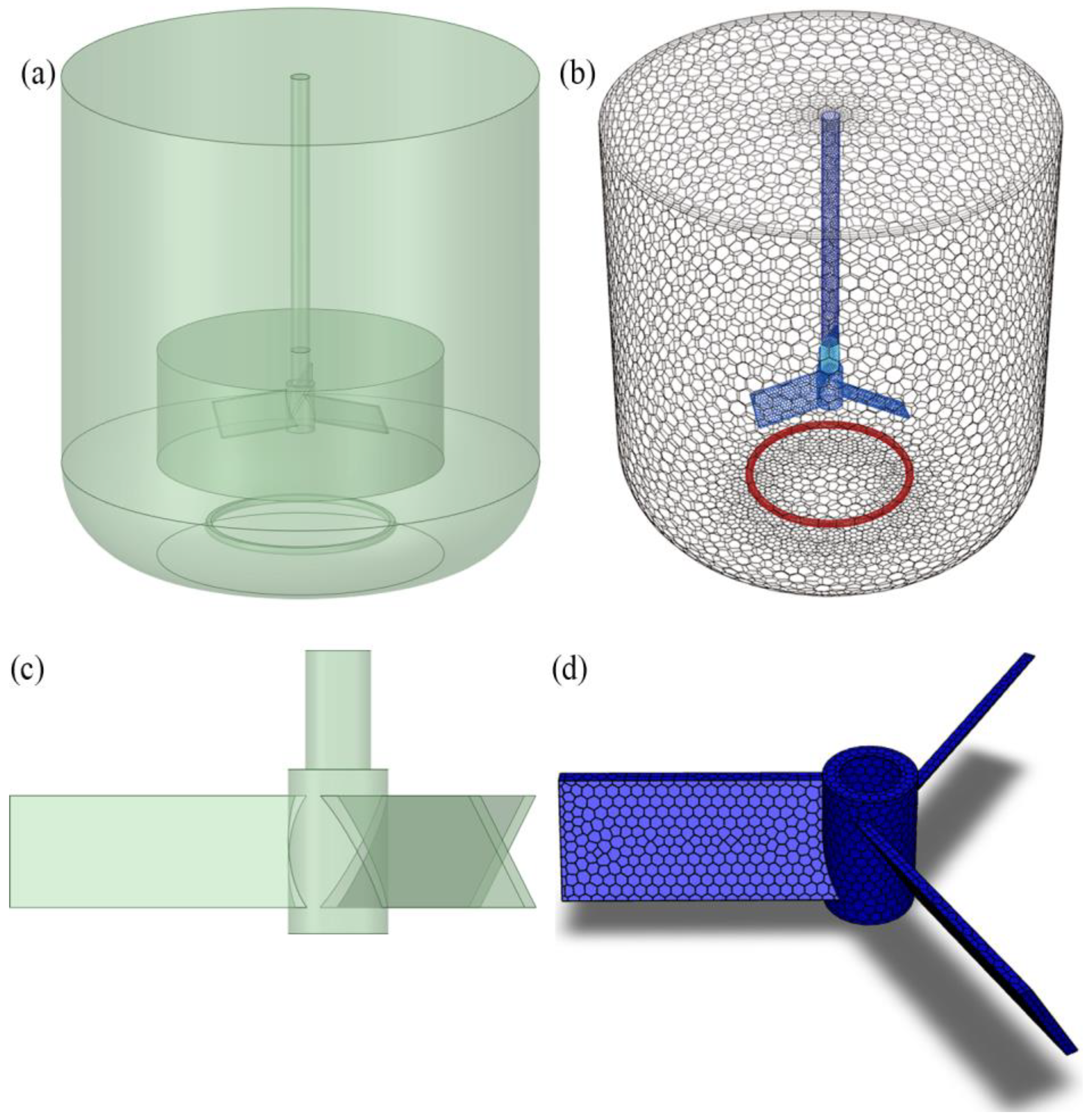
In this work, SpaceClaim is used for modeling, and the computational domain is shown in Figure 1a. During modeling, the autoclave body is split into the main fluid domain and the stirring fluid domain, and the BOI geometry is constructed at the stirring fluid domain to encrypt the stirring fluid region locally. The structural parameters are shown in Table 1. The type of impeller is a pitched blade turbine, which is the most commonly used axial flow impeller and is widely used in multiphase circulating mixing systems such as those in biology, metallurgy, and the chemical industry. The meshing is performed by the fluent meshing model, and the grid scheme is poly-hexcore [37]. This grid type employs a hybrid grid configuration and it has the advantage of drastically reducing the number of cells and conserving computational resources. The final generated mesh is shown in Figure 1b. The geometric construction of the pitched blade turbine and the generated mesh are shown in Figure 1c and Figure 1d, respectively.
3.2. Boundary Conditions
In this work, the MRF (multiple reference frame) method is used [38,39] for the rotation modeling, and the dynamic and static regions are calculated using different reference frames. This method considers the impeller and its surrounding area to be a moving area, whereas the rest of the tank is considered to be a static area. The transport equations in different regions of the MRF method are separately solved, and information transfer at the region boundaries is taken into account. The tank walls and impeller surfaces were treated as no-slip boundaries with standard wall functions. The gas enters the domain of fluids via the gas sparger and the speed is controlled to be 1 × 10⁻⁶ kg/s. The diameter of solid particles is controlled to be 0.002 m, and the density is 2000 kg/m3. Both solid–liquid and gas–liquid simulations have pressure conditions of 1 MPa.
In solid–liquid multiphase flow simulations, only the Schiller–Naumann drag is considered. The SIMPLE algorithm was used for pressure–velocity coupling. In addition, the first-order upwind discretization scheme was applied for convection terms. Due to the low density of the gas phase and the significant difference between it and the density of water, the bubble–particle phase of the gas–liquid simulation must account for the Saffman lift force and the pressure gradient force. The phase-coupled SIMPLE method was used to solve the coupling between pressure and velocity. The calculation is transient, time step is 0.01 s, and convergence residual variable is set to 10−4. All calculations were run on the same workstation, which included a 3.0-GHz CPU (AMD Ryzen Threadripper 2990WX 32-Core Processor) and 64 GB of RAM.
4. Results and Discussion
4.1. Grid Independence
While a smaller grid discretization error results in more precise simulations, it also requires more processing power and slows down convergence. In general, it is required to strike a balance between computation precision and calculation amount, and grid independence verification is used to determine the ideal number of grids [40]. The fundamental concept is to create a compromise between calculation accuracy and grid number by evaluating the deviation of a variable under different grid numbers of models under different grid number variables. In this work, the averaged flow field velocities near the impeller tip are compared using different grid numbers while all other variables remain unchanged. All simulations were carried out at N = 150 rpm. The flow field velocity changes for five grid numbers are shown in Table 2. As the number of grids increases, the change in the velocity of the flow field decreases gradually. Considering the computational cost issue, the grid finally adopts solution 3.
4.2. Experimental Verification
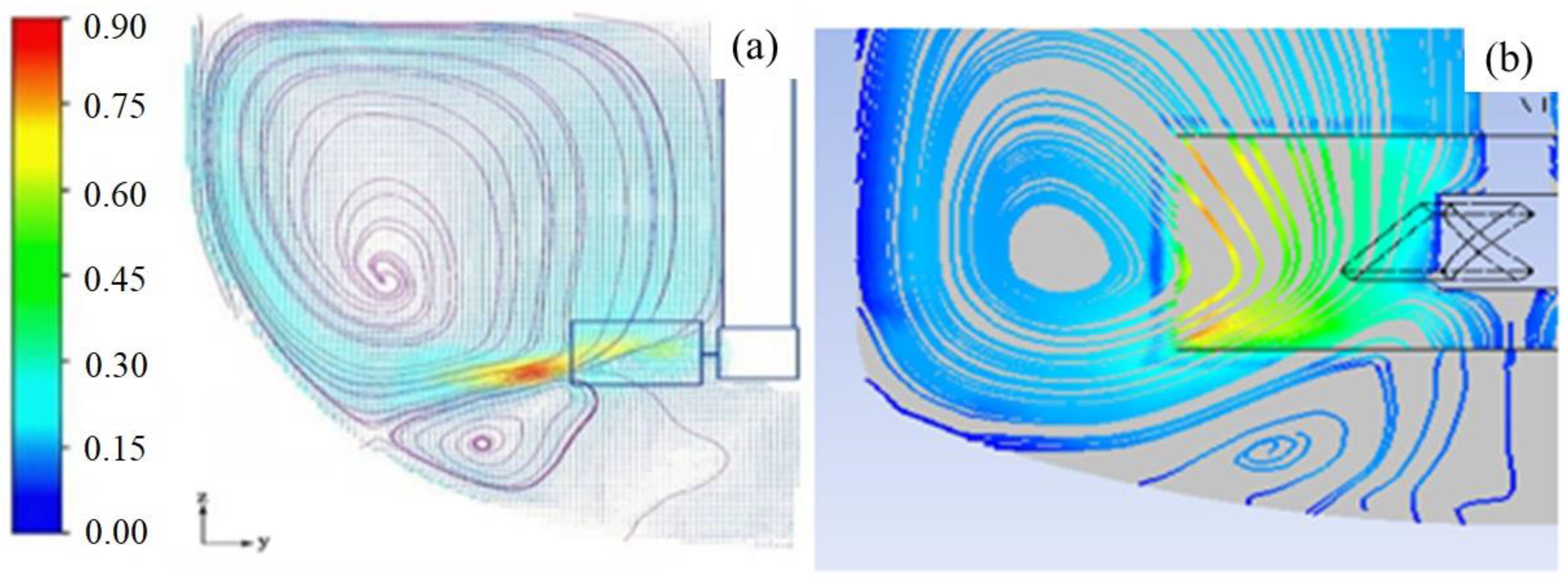
This work uses PIV [41] technology to experimentally verify the computational model. The equipment used is the PIV system produced by TSI Company in the United States, which consists of four parts: a tracer particle adding device, a double-pulse laser+ light sheet system, a CCD camera, and an information processing system. Through preliminary experiments on various impeller speeds and different planes, the stirring speed was selected as 150 rpm, and the exposure time delay was determined to be 1000 μs. The tracer uses a PSP tracer with a diameter of 50 μm, which is close to the density of water and has good followability and stability. The velocity component is calculated by DANTEC software, the captured image is set as a query area of 32 × 32 pixels, and the data of 200 images is time-averaged to obtain a reasonable velocity flow field. Comparing the PIV experimental data with the CFD simulation results, the streamline is shown in Figure 2.
The simulation-predicted value and the experimental value of the liquid velocity are compared in Figure 3. It can be observed that the simulation results of the CFD model are reliable and in good agreement with the experimental data.
4.3. Solid Holdup Distribution
Figure 4 shows the volume fraction distribution of the solid phase in the autoclave at different times when the stirring speed is 200 rpm. It is clear that the axial flow in the autoclave has the greatest influence on solid-phase dispersion, and the solid phase diffuses with the large circulating flow above the blades. Because of the impact of the blade jet, the solid phase diffuses to the upper section of the autoclave body in the first 4 s. Within 4–8 s, the solid-phase particles are affected by the large circulating flow above the autoclave and spread throughout the autoclave body. After about 10 s, the solid-phase distribution in the autoclave reached the stable state. Due to the low stirring speed, there was some solid-phase accumulation and insufficient solid-phase dispersion at the bottom of the autoclave after the steady state was reached. The volume fraction of most of the solid phase in the autoclave was about 2.2%.
Figure 5 shows the volume fraction distribution of the solid phase in the autoclave when the system reaches a steady state under different agitation speed conditions. When the speed is low (200 rpm to 300 rpm), solid-phase deposition occurs at the bottom of the autoclave and the solid-phase distribution above the autoclave is low, resulting in poor mixing. When the rotational speed was increased to 400 rpm, the solid-phase distribution in the autoclave became uniform, and the solid-phase distribution in the upper portion improved. When the stirring speed was increased to 500 rpm and 600 rpm, the accumulation of solid-phase suspensions appeared above the autoclave. This is due to the high turbulent kinetic energy in the autoclave caused by the high stirring speed. The lift force generated by the mainstream axial flow in the autoclave is large, and the solid phase is back-accumulated in the lower flow rate area above the autoclave.
In order to describe the solid-phase distribution inside the autoclave more visually, the solid-phase volume distribution at different locations inside the autoclave was monitored. Figure 6a is the solid-phase volume fraction curve in the horizontal direction at the Y = 0 section at the bottom of the autoclave. When the stirring speed is low, the volume fraction of the solid phase at the bottom of the autoclave will peak, which indicates that there is an accumulation of solid phase at the bottom of the autoclave. When the agitation speed is high, however, the solid holdup at the autoclave’s bottom tends to be uniform, and the phase volume fraction decreases. Due to the high speed, the majority of solids in the autoclave gather above the impeller.
Figure 6b is the solid-phase volume fraction curve in the axial direction at r = 0.3 m on the Y = 0 section. When the stirring speed is low (200 rpm to 300 rpm), the volume fraction of the solid phase increases and the part of the solid holdup in the autoclave decreases. The volume percentage of the solid phase above the autoclave grows as the rotation speed increases, and a peak appears at Z = 0.8 m, suggesting that the solid-phase aggregates at this position and the overall solid holdup uniformity in the autoclave declines, which is not conducive to mixed flow.
4.4. Critical Suspension Speed
The critical suspension speed is an important basis for judging the solid–liquid dispersion performance of the autoclave. It was first proposed by Zwietering [42], and it is also the most ideal operating condition for the autoclave. In general, the critical suspension speed is determined by the speed at which the solid phase remains at the bottom for less than 12 s. The empirical formula is as shown in Equation (14). We determined the average solid volume fraction at the Z = 0.05 m level at the bottom of the autoclave at 200 rpm, 300 rpm, 400 rpm, 500 rpm, and 600 rpm, respectively, by examining the distribution of the solid holdup at the bottom of the autoclave at various speeds. The critical suspension speed corresponds to the junction of the two tangents, which is drawn at the maximum slope and the minimum slope of the curve. Figure 7 is a schematic diagram for judging the critical suspension agitation speed under different agitation speed conditions.
With the increase in stirring speed, the average solid-phase volume fraction in the bottom area of the autoclave decreased. Then, make the maximum slope and the minimum slope tangent, and from the figure, it can be found that the coordinates of the intersection point O is (406, 0.0322). Therefore, the critical suspension speed of the autoclave is Nsp = 406 rpm. Take the shape factor of the autoclave as K = 1.4, the solid-phase particle density is 2000 kg/m3, the diameter is 0.1 mm, the solid holdup is Cv = 0.042, the blade diameter is 0.1 m, and the dynamic viscosity of water is 1.005 × 10⁻³ N∙s/m2. After calculation, the result obtained is Njs = 432 rpm, which is slightly higher than the simulated data.
4.5. Nonuniformity of Solid Suspension
Under actual working conditions, there are velocity and pressure differences in the flow field inside the autoclave, and the solid–liquid distribution cannot be completely uniform. Calculating the homogeneity of solid-phase dispersion is one of the criteria used to judge the quality of multi-phase mixing in the autoclave. The more uniform the solid-phase dispersion, the better the autoclave’s stirring effect and the more conducive mass transfer between phases. Take 5 positions of Z = 0.1 m, 0.3 m, 0.5 m, 0.7 m, and 0.9 m in the Z direction of the autoclave section, and calculate the average solid-phase volume distribution at different positions. Then, use Equation (15) to calculate the inhomogeneity of the solid-phase distribution at this speed. Take a stirring speed of 500 rpm as an example. Figure 8a is the solid-phase volume fraction curve at different horizontal positions of the Y = 0 section of the autoclave when the stirring speed of the autoclave is 500 rpm. With the increased position of the autoclave, the volume distribution of the solid phase shows an increasing trend, and the volume fraction of the solid phase is the highest at Z = 0.7 m, while the solid-phase content decreases near the stirring axis.
where αi is local solid holdup and α is the average solid holdup of the autoclave.
The inhomogeneity of the solid-phase suspension at the stirring speed is determined by calculating the average solid-phase volume fraction corresponding to each curve. Figure 8b shows the calculated suspension unevenness at different agitation speeds. In the autoclave, as the stirring speed increased, the non-uniformity of the solid-phase suspension first decreased and subsequently increased. At N = 400 rpm, the inhomogeneity of the solid-phase suspension is the lowest (σ = 8.65 × 10⁻²), the solid–liquid mixing in the autoclave is the most uniform, and the stirring effect is the best.
4.6. Gas Holdup Distribution
The impeller we use is a typical axial-flow impeller. During the ascent of the gas phase, it will interact with the blade jet in the blade region. When the stirring speed is high, the shear force generated by the blade jet is large, and the gas phase will diffuse to the bottom of the autoclave under the influence of drag force before ascending along the wall. Figure 9 shows the distribution of gas holdup in the autoclave at different stirring speeds.
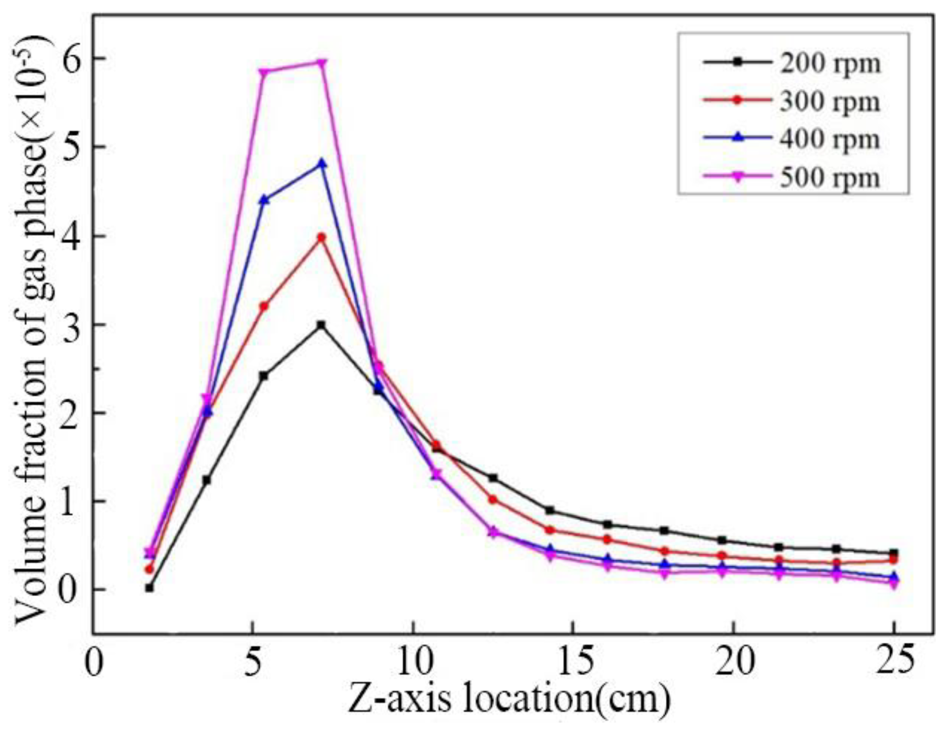
When the stirring speed is N = 100 rpm, the air bubbles are less affected by the blade jet. The gas phase distribution is a transition state between the gas flooding state and the remaining carrier gas state and is only partially affected by the flow field. The effect of phase separation and dispersion is poor, and there is a phenomenon of gas aggregation in the vortex area of the blade, which is not conducive to gas phase diffusion and mass transfer. When the stirring speed was increased to 300 rpm, however, the autoclave’s gas phase was entirely dispersed. Under the action of the blade jet, the gas phase is spread throughout the entire autoclave body, the distribution is more uniform, and the range of the dead zone is reduced. Figure 10 shows the gas phase distribution curve in the axial direction of the autoclave at different stirring speeds. With the increase in agitation speed, the overall gas holdup in the autoclave increases. This is due to the existence of circulation in the gas phase. The residence time thus becomes longer, and the gas–liquid mixing effect is good. In addition, the gas phase is mostly concentrated in the flow field’s vortex core region. As the blade speed increases, the gas phase concentration in the vortex core region becomes more apparent.
4.7. Bubble Tracks and Residence Time
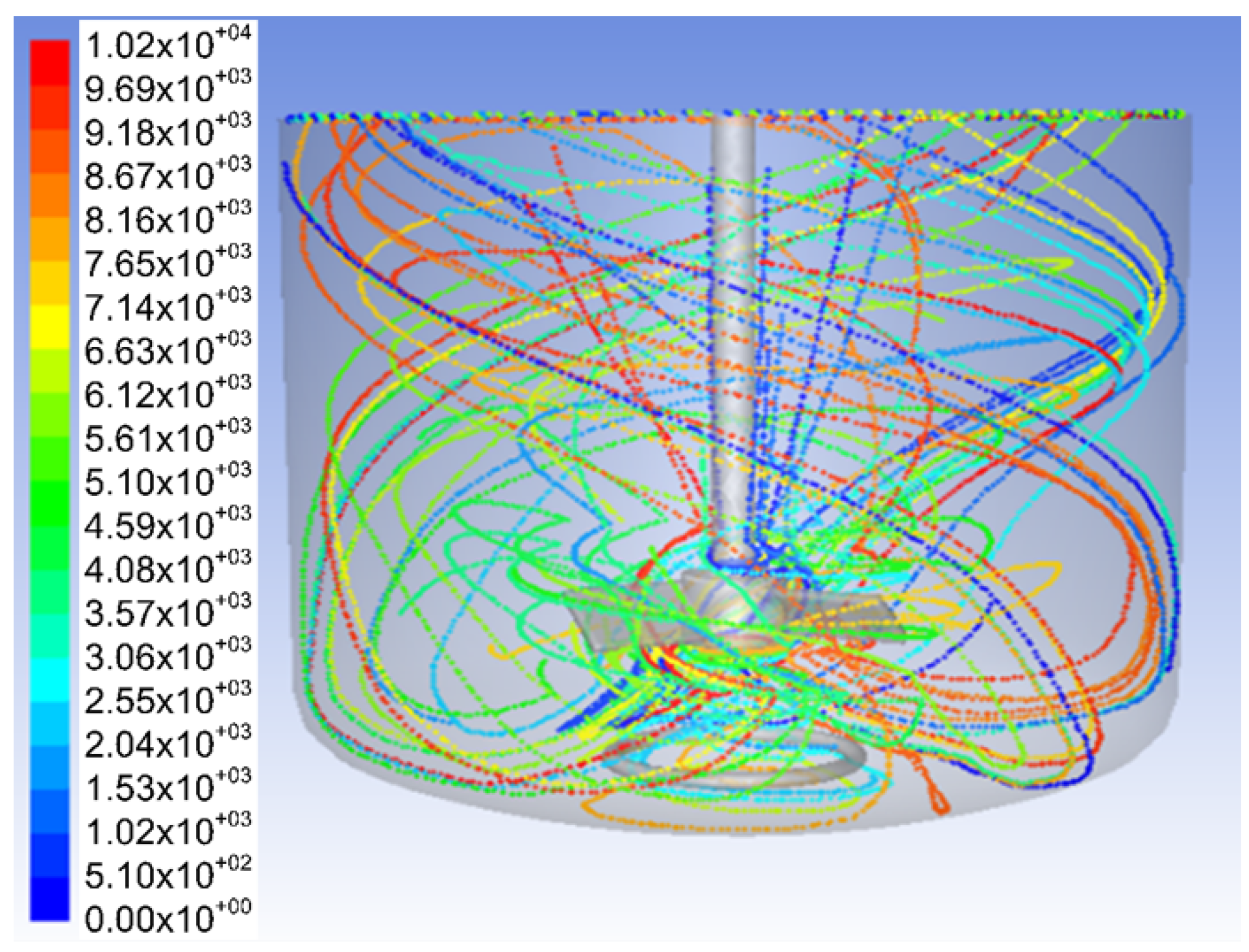
The DPM obtains the particle tracks by calculating the force balance and motion equation of each particle phase. Figure 11 shows the trajectory of the bubble movement in the autoclave when the stirring speed is N = 400 rpm. Via monitoring of the overall gas holdup, it is determined that the flow field has achieved a steady state when the bubble dispersion time is 5.6 s. However, once the flow field had stabilized, we proceeded to observe bubble dispersion to determine the maximum bubble residence time. When the agitation speed is high, the bubble movement is mainly affected by the drag force. The bubbles are introduced by the ring sparger and propelled by the blade’s jet during the ascent process. Under the influence of flow field drag, they rotate around the axis. Under the influence of the axial flow blade, gas phase diffusion is comparatively adequate. The gas phase will diffuse to the bottom of the autoclave and all parts of the autoclave due to the action of axial flow, and the overall gas–liquid dispersion effect of the autoclave is improved.
The bubble residence time evaluates the autoclave’s gas phase circulation performance, which has a direct impact on the gas–liquid mass transfer time. This is carried out by capturing the bubble particles that reach the top of the autoclave under different stirring speeds and counting their particle information to obtain the bubble residence time at different agitation speeds, as shown in Table 3. With the increase in stirring speed, the minimum residence time of bubbles decreases and the maximum residence time increases. This is due to the growing impact of turbulence on bubble movement and the increase in residence time variation. It demonstrates that the regularity of bubble residence time distribution is diminished and that the residence time is affected by high dispersion of turbulent shear. The average residence time of bubbles increases with the increase in agitation speed, which is conducive to gas phase dispersion and mass transfer. At 300 and 400 rpm, the bubble residence time is closer. This is due to the fact that the gas phase has reached a condition of complete dispersion, and increasing the agitation speed has little influence on the dispersion of the gas phase.
Figure 12 shows the distribution of bubble particles in the autoclave at different times. When t = 2 s, the bubble particles had just arrived at the blade area and were starting to disperse under the influence of the blade jet; when t = 4 s, the bubbles had diffused throughout the autoclave, and a small amount of bubble particles began to overflow. When t = 6 s, the bubble particles further increased, the overall concentration of bubble particles above the autoclave increased, and the phenomenon of bubble particle circulation began to appear. When t = 8 s, the phase of bubble particles increases, and the particles with a higher residence time mainly appear in the area near the stirring shaft. This may be due to the fact that this portion of the region is the recirculation region of some major circulations on the flow field, and some bubbles have circulating diffusion in this region. In addition to slowing the ascent of bubble particles, the recirculation zone increases the bubbles’ residence time in this region.
The particles are captured on the pressure outlet boundary of the autoclave, and the residence time distribution of the bubble particles can be quantitatively calculated using statistical particle information (Figure 13). We counted the residence time of some particles. The residence time distribution of the bubble particles shows a tailing phenomenon, and the peak value of the residence time appears at t = 5 s.
5. Conclusions
In this work, a multiphase flow model was used to simulate the multiphase mixing characteristics in the autoclave. The simulation studies on the solid–liquid mixing characteristics and gas–liquid dispersion in the autoclave were carried out, respectively. The conclusions are as follows:
- (1)
- The solid-phase volume distribution clouds were analyzed at different times. The solid–liquid mixing was greatly influenced by the axial flow of the autoclave. The solid-phase deposition at the bottom of the autoclave decreased as the stirring speed increased. The solid-phase distribution in the autoclave became more uniform when the rotation speed was increased to 400 rpm. If the agitation speed is increased again, the phenomenon of solid-phase accumulation above the autoclave will arise, which is not conducive to solid-phase dispersion and mass transfer in the autoclave, and the autoclave’s power consumption will increase.
- (2)
- At various speeds, the average solid-phase volume fraction at the bottom of the autoclave is used to determine the critical suspension speed of solid–liquid mixing. After processing and calculating the simulated data, Nsp = 406 rpm was found to be the critical suspension speed for mixing solids and liquids in the autoclave. Its value is marginally lower than the critical suspension speed calculated using the empirical equation. By examining the suspension inhomogeneity at various stirring speeds, the solid-phase suspension inhomogeneity exhibited a decreasing and subsequently increasing pattern. The nonuniformity of the solid suspension is lowest when the stirring speed is 400 rpm (σ = 8.65 × 10⁻²).
- (3)
- The contours of the volume distribution of the gas phase in the autoclave under various agitation speed conditions were examined. The gas phase dispersion in the autoclave is totally diffused at 300 rpm stirring speed. With the increase in agitation speed, the gas content of the autoclave increases, and the gas phase is mainly concentrated in the vortex area above the blades.
- (4)
- Analysis was conducted on the bubble tracks and residence time. The drag force of the flow field mostly influences the movement of the bubbles. In the vicinity of the agitator shaft, air bubbles remain longer in the fluid recirculation zone. At the exit, we measured the time of bubble residence. The average bubble residence time increases as stirring speed increases. When the gas phase is in a completely dispersed state (N = 300 rpm), the average bubble residence time is 5.66 s, and increasing the stirring speed cannot effectively improve the gas phase residence time.
Author Contributions
Conceptualization, Y.H. and G.X.; methodology, B.K. and Y.H.; software, Y.H.; validation, B.K., Y.H. and N.Y.; formal analysis, W.F.; investigation, J.L.; resources, G.X.; data curation, B.K.; writing—original draft preparation, B.K.; writing—review and editing, Y.H.; visualization, B.K.; supervision, Y.H.; project administration, Y.H.; funding acquisition, Y.H. All authors have read and agreed to the published version of the manuscript.
Funding
This work was supported in part by National Natural Science Foundation of China (Project Nos. 52074141,22168019).
Data Availability Statement
The data presented in this study are available on request from the corresponding author.
Conflicts of Interest
The authors declare no conflict of interest.
References
- Loveday, B.K. The use of oxygen in high pressure acid leaching of nickel laterites. Miner. Eng. 2008, 21, 533–538. [Google Scholar] [CrossRef]
- Lewis, W.K.; Whitman, W.G. Principles of Gas Absorption. Ind. Eng. Chem. 1924, 16, 1215–1220. [Google Scholar] [CrossRef]
- Puthli, M.S.; Rathod, V.K.; Pandit, A.B. Gas-liquid mass transfer studies with triple impeller system on a laboratory scale bioreactor. Biochem. Eng. J. 2005, 23, 25–30. [Google Scholar] [CrossRef]
- Fadavi, A.; Chisti, Y. Gas–liquid mass transfer in a novel forced circulation loop reactor. Chem. Eng. J. 2005, 112, 73–80. [Google Scholar] [CrossRef]
- Ramezani, M.; Kong, B.; Gao, X.; Olsen, M.G.; Vigil, R.D. Experimental measurement of oxygen mass transfer and bubble size distribution in an air–water multiphase Taylor–Couette vortex bioreactor. Chem. Eng. J. 2015, 279, 286–296. [Google Scholar] [CrossRef] [Green Version]
- Lee, J.; Yasin, M.; Park, S.; Chang, I.S.; Ha, K.-S.; Lee, E.Y.; Lee, J.; Kim, C. Gas-liquid mass transfer coefficient of methane in bubble column reactor. Korean J. Chem. Eng. 2015, 32, 1060–1063. [Google Scholar] [CrossRef]
- Henrique, S.; Edgar, M.O.; Sergio, C.; Rigoberto, E.M.M. Numerical assessment of performance characteristics and two-phase flow dynamics of a centrifugal rotor operating under gas entrainment condition. Exp. Comput. Multiph. Flow 2022, 4, 221–240. [Google Scholar] [CrossRef]
- Masterov, M.V.; Baltussen, M.W.; Kuipers, J.A.M. Numerical simulation of a square bubble column using Detached Eddy Simulation and Euler–Lagrange approach. Int. J. Multiph. Flow 2018, 107, 275–288. [Google Scholar] [CrossRef]
- Sommer, A.; Rox, H.; Shi, P.; Eckert, K.; Rzehak, R. Solid-liquid flow in stirred tanks: “CFD-grade” experimental investigation. Chem. Eng. Sci. 2021, 245, 116743. [Google Scholar] [CrossRef]
- Zhang, C.; Yang, F. Gas-liquid mixing in the stirred tank equipped with semi-circular tube baffles. Int. J. Chem. React. Eng. 2022. [Google Scholar] [CrossRef]
- Hu, X.; Ilgun, A.D.; Passalacqua, A.; Fox, R.O.; Bertola, F.; Milosevic, M.; Visscher, F. CFD simulations of stirred-tank reactors for gas-liquid and gas-liquid-solid systems using OpenFOAM®. Int. J. Chem. React. Eng. 2021, 19, 193–207. [Google Scholar] [CrossRef]
- Maluta, F.; Paglianti, A.; Montante, G. Two-fluids RANS predictions of gas cavities, power consumption, mixing time and oxygen transfer rate in an aerated fermenter scale-down stirred with multiple impellers. Biochem. Eng. J. 2021, 166, 107867. [Google Scholar] [CrossRef]
- Ramírez-Torres, L.A.; Medina-Torres, L.; Calderas, F.; Núñez-Ramírez, D.M.; Manero, O. Rheology and Hydrodynamics of Iron Ore Mineral Pulps during a Bioleaching Process in a Continuous Stirred-Tank Reactor. Chem. Eng. Technol. 2022, 46, 1–12. [Google Scholar] [CrossRef]
- Gu, D.; Wen, L.; Xu, H.; Ye, M. Study on hydrodynamics characteristics in a gas-liquid stirred tank with a self-similarity impeller based on CFD-PBM coupled model. J. Taiwan Inst. Chem. Eng. 2023, 143, 104688. [Google Scholar] [CrossRef]
- Cheng, D.; Wang, S.; Yang, C.; Mao, Z.-S. Numerical Simulation of Turbulent Flow and Mixing in Gas–Liquid–Liquid Stirred Tanks. Ind. Eng. Chem. Res. 2017, 56, 13050–13063. [Google Scholar] [CrossRef] [Green Version]
- García-Hernández, E.; Aguilar-Madera, C.; Herrera-Hernández, E.; Flores-Cano, J.; Bailón-García, E.; González, A.; Aguilar-Aguilar, A.; Ocampo-Pérez, R. 3D Modeling of the Adsorption Rate of Pyridine on Activated Carbon Cloth in a Stirred Tank under Turbulent Conditions. Processes 2022, 10, 735. [Google Scholar] [CrossRef]
- Fan, Y.; Sun, J.; Jin, J.; Sun, K.; Zhang, H.; Chen, W.; Li, Y. Effects of baffle on flow structure and cyclic variation in stirred tanks with Rushton turbine. AIP Adv. 2022, 12, 015202. [Google Scholar] [CrossRef]
- Verzicco, R.; Fatica, M.; Iaccarino, G.; Orlandi, P. Flow in an impeller-stirred tank using an immersed-boundary method. AIChE J. 2004, 50, 1109–1118. [Google Scholar] [CrossRef]
- Martinez, L.; Duret, B.; Reveillon, J.; Demoulin, F. Vapor mixing in turbulent vaporizing flows. Int. J. Multiph. Flow 2023, 161, 104388. [Google Scholar] [CrossRef]
- Mochalin, I.; Cai, J.; Shiju, E.; Brazhenko, V.; Wang, D. Numerical study of the flow through an annular gap with filtration by a rotating porous cylinder. Eng. Appl. Comput. Fluid Mech. 2022, 16, 469–483. [Google Scholar] [CrossRef]
- Piomelli, U.; Balaras, E. Wall-Layer Models for Large-Eddy Simulations. Annu. Rev. Fluid Mech. 2002, 34, 349–374. [Google Scholar] [CrossRef] [Green Version]
- Kahouadji, L.; Liang, F.; Valdes, J.; Shin, S.; Chergui, J.; Juric, D.; Craster, R.; Matar, O. The transition to aeration in turbulent two-phase mixing in stirred vessels. Flow 2022, 2, E30. [Google Scholar] [CrossRef]
- Bernauer, S.; Schöpf, M.; Eibl, P.; Witz, C.; Khinast, J.; Hardiman, T. Characterization of the gas dispersion behavior of multiple impeller stages by flow regime analysis and CFD simulations. Biotechnol. Bioeng. 2021, 118, 3058–3068. [Google Scholar] [CrossRef] [PubMed]
- Ling, J.; Kurzawski, A.; Templeton, J. Reynolds averaged turbulence modelling using deep neural networks with embedded invariance. J. Fluid Mech. 2016, 807, 155–166. [Google Scholar] [CrossRef]
- Islam, M.T.; Nguyen, A.V. Effect of microturbulence on bubble-particle collision during the bubble rise in a flotation cell. Miner. Eng. 2020, 155, 106418. [Google Scholar] [CrossRef]
- Varghese, M.M.; Vakamalla, T.R. Effect of Turbulence Model on the Hydrodynamics of Gas-solid Fluidized Bed. In Recent Trends in Fluid Dynamics Research; Bharti, R.P., Gangawane, K.M., Eds.; Springer Nature: Singapore, 2022; pp. 47–61. [Google Scholar] [CrossRef]
- Rollet-Miet, P.; Laurence, D.; Ferziger, J. LES and RANS of turbulent flow in tube bundles. Int. J. Heat Fluid Flow 1999, 20, 241–254. [Google Scholar] [CrossRef] [Green Version]
- Brazhenko, V.; Qiu, Y.; Mochalin, I.; Zhu, G.; Cai, J.-C.; Wang, D. Study of hydraulic oil filtration process from solid admixtures using rotating perforated cylinder. J. Taiwan Inst. Chem. Eng. 2022, 141, 104578. [Google Scholar] [CrossRef]
- Joulaei, A.; Nili-Ahmadabadi, M.; Ha, M.Y. Numerical study of the effect of geometric scaling of a fluidic oscillator on the heat transfer and frequency of impinging sweeping jet. Appl. Therm. Eng. 2023, 221, 119848. [Google Scholar] [CrossRef]
- Parikh, T.; Mansour, M.; Thévenin, D. Investigations on the effect of tip clearance gap and inducer on the transport of air-water two-phase flow by centrifugal pumps. Chem. Eng. Sci. 2020, 218, 115554. [Google Scholar] [CrossRef]
- Yang, X.; Yang, G.; Liu, P.; Li, X.; Jiang, L.; Zhang, J. Study on the Desliming Performance of a Novel Hydrocyclone Sand Washer. Separations 2022, 9, 74. [Google Scholar] [CrossRef]
- Coroneo, M.; Montante, G.; Paglianti, A.; Magelli, F. CFD prediction of fluid flow and mixing in stirred tanks: Numerical issues about the RANS simulations. Comput. Chem. Eng. 2011, 35, 1959–1968. [Google Scholar] [CrossRef]
- Tominaga, Y.; Stathopoulos, T. CFD Modeling of Pollution Dispersion in Building Array: Evaluation of turbulent scalar flux modeling in RANS model using LES results. J. Wind. Eng. Ind. Aerodyn. 2012, 104–106, 484–491. [Google Scholar] [CrossRef] [Green Version]
- Booth, C.P.; Leggoe, J.W.; Aman, Z.M. The use of computational fluid dynamics to predict the turbulent dissipation rate and droplet size in a stirred autoclave. Chem. Eng. Sci. 2018, 196, 433–443. [Google Scholar] [CrossRef]
- Mohammad, A.F.; Mourad, A.A.H.I.; Al-Marzouqi, A.H.; El-Naas, M.H.; Van der Bruggen, B.; Al-Marzouqi, M.H.; Alnaimat, F.; Al Musharfy, M. Comprehensive Optimization of the Dispersion of Mixing Particles in an Inert-Particle Spouted-Bed Reactor (IPSBR) System. Processes 2021, 9, 1921. [Google Scholar] [CrossRef]
- Li, Y.; Zhang, J.; Fan, L.-S. Numerical simulation of gas–liquid–solid fluidization systems using a combined CFD-VOF-DPM method: Bubble wake behavior. Chem. Eng. Sci. 1999, 54, 5101–5107. [Google Scholar] [CrossRef]
- Felekos, G.; Douvi, E.; Margaris, D. Cost-effective numerical analysis of the DrivAer fastback model aerodynamics. Proc. Inst. Mech. Eng. Part D J. Automobile Eng. 2022, 09544070221135908. [Google Scholar] [CrossRef]
- Patil, H.; Patel, A.K.; Pant, H.J.; Vinod, A.V. CFD simulation model for mixing tank using multiple reference frame (MRF) impeller rotation. ISH J. Hydraul. Eng. 2021, 27, 200–209. [Google Scholar] [CrossRef]
- Maluta, F.; Paglianti, A.; Montante, G. Prediction of gas cavities size and structure and their effect on the power consumption in a gas-liquid stirred tank by means of a two-fluid RANS model. Chem. Eng. Sci. 2021, 241, 116677. [Google Scholar] [CrossRef]
- Cloete, S.; Johansen, S.T.; Amini, S. Grid independence behaviour of fluidized bed reactor simulations using the Two Fluid Model: Detailed parametric study. Powder Technol. 2016, 289, 65–70. [Google Scholar] [CrossRef] [Green Version]
- Gecim, G.; Erkoc, E. Gas Flow Hydrodynamics in Vortex Mixers: Flow Visualization and PIV Flow Field Characterization. Ind. Eng. Chem. Res. 2021, 60, 5674–5687. [Google Scholar] [CrossRef]
- Zwietering, T.N. Suspending of solid particles in liquid by agitators. Chem. Eng. Sci. 1958, 8, 244–253. [Google Scholar] [CrossRef]
Figure 1.
(a) Computational domain; (b) generated mesh; (c) pitched blade turbine; (d) generated mesh of impeller.
Figure 1.
(a) Computational domain; (b) generated mesh; (c) pitched blade turbine; (d) generated mesh of impeller.

Figure 2.
The streamline diagram of PIV (a) and CFD (b).

Figure 3.
Z-axis direction liquid phase velocity distribution.

Figure 4.
Volume fraction distribution of solid phase at N = 200 rpm. (a) t = 0 s; (b) t = 2 s; (c) t = 4 s; (d) t = 6 s; (e) t = 8 s; (f) t = 10 s.
Figure 4.
Volume fraction distribution of solid phase at N = 200 rpm. (a) t = 0 s; (b) t = 2 s; (c) t = 4 s; (d) t = 6 s; (e) t = 8 s; (f) t = 10 s.

Figure 5.
Solid phase volume fraction distribution at steady state. (a) N = 200 rpm; (b) N = 300 rpm; (c) N = 400 rpm; (d) N = 500 rpm; (e) N = 600 rpm.
Figure 5.
Solid phase volume fraction distribution at steady state. (a) N = 200 rpm; (b) N = 300 rpm; (c) N = 400 rpm; (d) N = 500 rpm; (e) N = 600 rpm.

Figure 6.
(a) Solid phase volume fraction distribution at different agitation speeds; (b) solid volume fraction distribution at different agitation speeds.
Figure 6.
(a) Solid phase volume fraction distribution at different agitation speeds; (b) solid volume fraction distribution at different agitation speeds.

Figure 7.
Average solid volume fraction at the bottom of the autoclave.

Figure 8.
(a) Solid volume fraction distribution at different horizontal positions; (b) the nonuniformity of solid suspension at different agitation speeds.
Figure 8.
(a) Solid volume fraction distribution at different horizontal positions; (b) the nonuniformity of solid suspension at different agitation speeds.

Figure 9.
Gas holdup contour. (a) N = 100 rpm; (b) N = 200 rpm; (c) N = 300 rpm; (d) N = 400 rpm.

Figure 10.
Axial distribution of gas phase volume fraction.

Figure 11.
Bubble tracks at N = 400 rpm.

Figure 12.
The bubble particle distribution in the autoclave. (a) t = 2 s; (b) t = 4 s; (c) t = 6 s; (d) t = 8s.
Figure 12.
The bubble particle distribution in the autoclave. (a) t = 2 s; (b) t = 4 s; (c) t = 6 s; (d) t = 8s.

Figure 13.
Bubble residence time.


Table 1.
Structural parameters of autoclave.
| Structure Parameters | Value | Structure Parameters | Value |
|---|---|---|---|
| Tank height | 26 cm | Diameter of ring sparger | 19.2 cm |
| Diameter of autoclave | 25 cm | Width of outlet | 0.23 cm |
| Bottom ellipse height | 5 cm | Blade width | 1.7 cm |
| Diameter of impeller | 10 cm | Blade thickness | 0.17 cm |
| Axial location of impeller | 6.8 cm | Chord angel | 30° |
Table 2.
Grid independence analysis.
| Grid Solutions | Mesh Number | Velocity (m/s) |
|---|---|---|
| Solution 1 | 264,853 | 0.56 |
| Solution 2 | 373,245 | 0.61 |
| Solution 3 | 422,658 | 0.74 |
| Solution 4 | 456,258 | 0.75 |
| Solution 5 | 468,523 | 0.75 |
Table 3.
Bubble residence time at different agitation speeds.
| Agitation Speed (rpm) | Minimum Residence Time (s) | Maximum Residence Time (s) | Average Residence Time (s) | Variance |
|---|---|---|---|---|
| 100 | 1.56 | 10.16 | 5.03 | 1.89 |
| 200 | 1.45 | 10.30 | 5.24 | 2.07 |
| 300 | 1.37 | 11.13 | 5.66 | 2.18 |
| 400 | 1.34 | 11.28 | 5.75 | 2.22 |
Disclaimer/Publisher’s Note: The statements, opinions and data contained in all publications are solely those of the individual author(s) and contributor(s) and not of MDPI and/or the editor(s). MDPI and/or the editor(s) disclaim responsibility for any injury to people or property resulting from any ideas, methods, instructions or products referred to in the content. |
© 2023 by the authors. Licensee MDPI, Basel, Switzerland. This article is an open access article distributed under the terms and conditions of the Creative Commons Attribution (CC BY) license (https://creativecommons.org/licenses/by/4.0/).
Share and Cite
MDPI and ACS Style
Kou, B.; Hou, Y.; Fu, W.; Yang, N.; Liu, J.; Xie, G. Simulation of Multi-Phase Flow in Autoclaves Using a Coupled CFD-DPM Approach. Processes 2023, 11, 890. https://doi.org/10.3390/pr11030890
AMA Style
Kou B, Hou Y, Fu W, Yang N, Liu J, Xie G. Simulation of Multi-Phase Flow in Autoclaves Using a Coupled CFD-DPM Approach. Processes. 2023; 11(3):890. https://doi.org/10.3390/pr11030890
Chicago/Turabian StyleKou, Bin, Yanqing Hou, Weiqin Fu, Ni Yang, Junchang Liu, and Gang Xie. 2023. "Simulation of Multi-Phase Flow in Autoclaves Using a Coupled CFD-DPM Approach" Processes 11, no. 3: 890. https://doi.org/10.3390/pr11030890
Note that from the first issue of 2016, this journal uses article numbers instead of page numbers. See further details here.