
Design and Comparison of Strategies for Level Control in a Nonlinear Tank


Electrical Engineering Department, Faculty of Engineering, University of Santiago of Chile (USACH), Av. Ecuador 3519, Estación Central, Santiago 9170124, Chile
*
Author to whom correspondence should be addressed.
Processes 2021, 9(5), 735; https://doi.org/10.3390/pr9050735
Submission received: 18 February 2021
/
Revised: 15 April 2021
/
Accepted: 20 April 2021
/
Published: 22 April 2021
Abstract
:In this work, a study of the water level control of an inverted conical tank system is presented. This type of tank has highly nonlinear mathematical and dynamic characteristics. Four control strategies are designed, applied, and compared, namely classical Proportional–Integral–Derivative (PID), Gain Scheduling (GS), Internal Model Control (IMC), and Fuzzy Logic (FL). To determine which of the designed control strategies are the most suitable for an inverted conical tank, a comparative study of the behavior of the system is carried out. With this purpose, and considering situations much closer to reality, a variety of scenarios, such as step responses, random input disturbances, and momentary load disturbances, are conducted. Additionally, performance indexes (error- and statistics-based) are calculated to assess the system’s response.
1. Introduction
Global climate change and the unpredictable rain cycle cause uncertainty in the availability of water. However, water is commonly used in homes, agriculture, and industry. Currently, one of the basic problems in industries is the water level control system. The liquid level, which is an important process parameter, must be kept at the desired level for the process to run smoothly and to obtain better-quality products. All process industries, water treatment plants, and nuclear power plants depend on the level control of tank systems. Many engineers have designed controllers based on linearized models of real tank systems. However, due to the complexity and nonlinearity of real processes, it is difficult to improve the performance of these real systems using conventional control techniques [1,2,3,4,5,6]. Therefore, it is vital that the engineers working in these systems, especially the control and mechatronics engineers, have a good understanding of how tank level control systems work and how difficult it is to handle level control.
Level control in tanks is a widespread need in industries from all sectors. In industrial processes, liquid level control in conical tanks is a major problem. For example, a level well above the surface can upset the process reaction balances and damage equipment, but a level below the required setpoint can also cause serious problems [7,8,9,10,11,12]. In particular, inverted conical tanks, the object of this study, exhibit significant operational advantages. For example, they allow for the reduction or elimination of sediments accumulated in the base of the tank, as well as the complete emptying of the same. However, the inherent nonlinearity of these tanks is considered a challenge for control systems [13,14,15,16,17,18].
Regarding level control in conical tanks, some studies introduce fractional-order internal model controllers, which have a fractional filter cascaded with an integer-order PID controller. In these cases, the linearization of the nonlinear systems includes the Lagrange remainder term to compensate for higher-order derivatives that are simulated using fractional-order PID and compared with classical PID and Gain-Scheduling PID [19,20]. In turn, different control techniques are used for the tank level controls, such as Backstepping, PI control by direct synthesis, and Gain Scheduling [21,22]. Some simulated comparisons between IMC, Model Predictive Control (MPC), and classical PID are presented in [23,24,25]. Additionally, results using a mix of fuzzy control and neural network control are presented in [26,27,28,29]. Other techniques for level control include Passive-Based Control (PBC), Linear Parameter Variation (LPV), and Particle Swarm Optimization (PSO) [7,19,30].
After reviewing the state of research on level control techniques for conical tanks, it has been found that in most publications, the level control is only simulated and/or implemented with changes in the reference, but without incorporating load variations or disturbances in the intake flow. Therefore, considering situations much closer to reality, load variations and disturbances are included in this work. To achieve this, four control strategies are designed, applied, and compared, namely classical PID, GS, IMC, and FL. To determine which of the designed control strategies are the most suitable for an inverted conical tank, a comparative study of the behavior of the system is carried out. With this purpose, a variety of scenarios, such as step responses, random input disturbances, and momentary load disturbances, are conducted. Additionally, performance indexes (error- and statistics-based) are calculated to assess the system’s response.
2. Description and Modeling of the System under Study
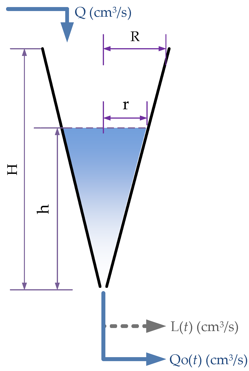
Figure 1 below shows the scheme of the tank under study.
A simulated tank was created for research purposes. This tank had an approximate capacity of 30 L and the following parameters, which are shown in Table 1.
The resulting approximate value for these parameters is 28.3 L. Therefore, the tank had a relatively small capacity. The analysis comprised a nonviscous fluid (for example, water, alcohol, fuel, etc.) at normal room-temperature conditions, and the tank was open in its upper part (nonpressurized). The usable level range of the simulated tank was set from 10 to 60 cm. The model variables, shown in Table 2, are:
L(t) is a dynamic variable for load disturbances. The input flow Q(t) was limited to 400 cm3/s, which is consistent with the mechanical capacity of the water pumps used for tanks of these dimensions.
2.1. Equation Model
To preserve liquid mass in the tank, it is established that:
where:
Substituting and solving (1), we obtain:
where . Substituting (4) into (1), and assuming that , the following is obtained:
Integrating (5), the nonlinear relation between input flow and level is obtained (considering ( = 0):
Load output will be considered null, except for specific simulations that require its use. Therefore, load output is not considered part of the general model of the tank. After applying such parameters, the constants and 7 are obtained.
2.2. Tank Linear Model
This work presents control simulations applied directly to the nonlinear model for the tank. However, for a number of applications such as PID tuning and implementation of IMC control, it is very useful to have a linear incremental model around a stationary level hs of the tank. This stationary level is related to the input flow QS.
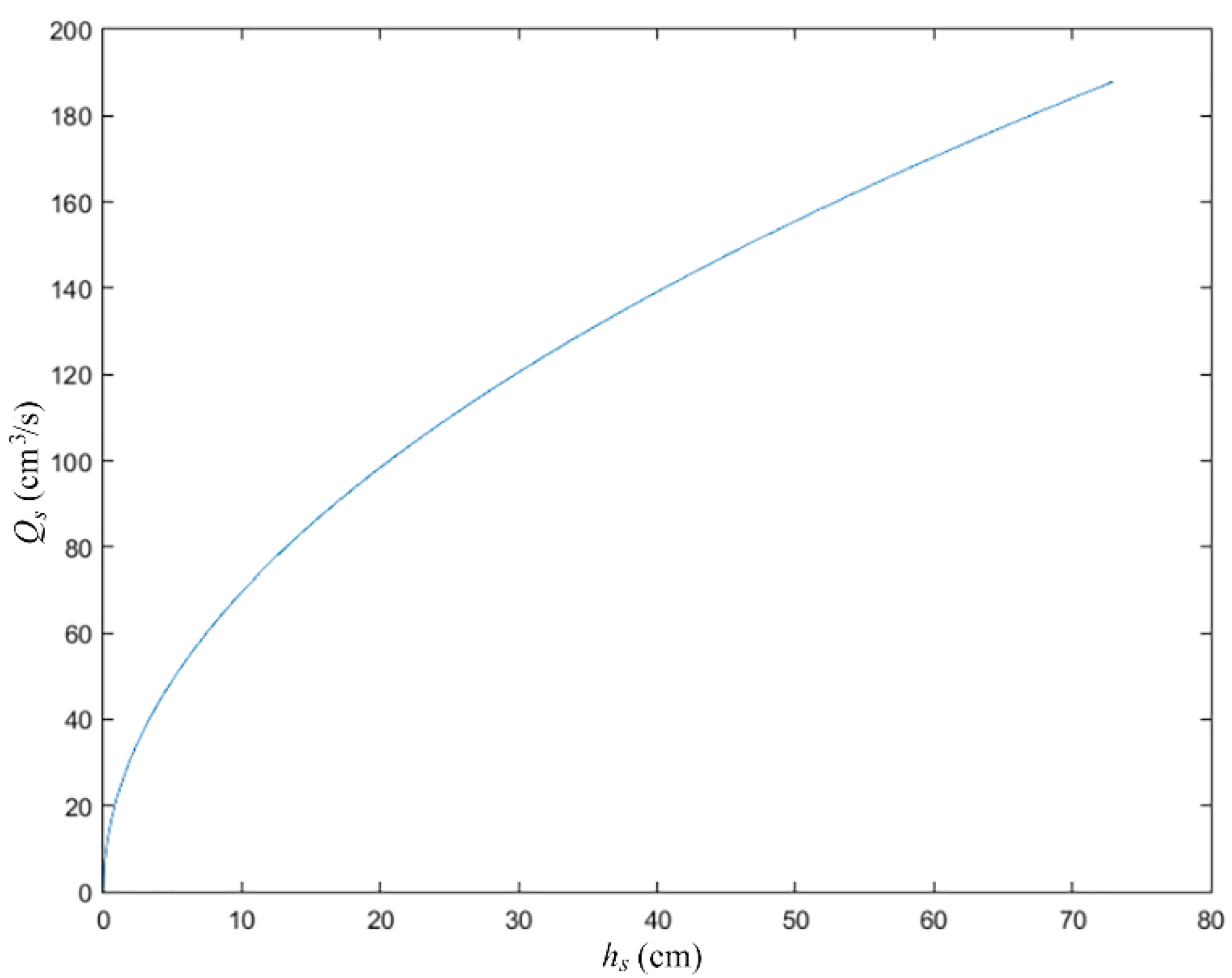
In practical terms, successfully controlling nonlinear systems in the vicinity of operation points is possible. In this case, for (,), when , solving (1) with = 0, we have:
The equation above allows us to generate a stationary state curve that links to , as shown in Figure 2.
A stationary operation point (,) is taken, and (5) is linearized around it, with = 0, by means of a Taylor series. Using the following changes of variables:
we obtain:
In the stationary state, . Substituting and reducing algebraically in the equation above, the following is obtained:
The objective is to reach the standard form of the equation , to then achieve the transfer function in the Laplace domain. Through the algebraic manipulation of (11), we obtain:
Resorting to the previous equation and simplifying after applying Laplace transform, we reach:
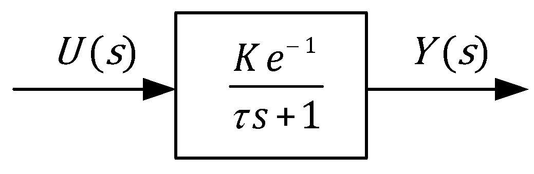
Equation (14) allows us to obtain an incremental linearized model for any stationary level, considering that terms and α are part of the system parameters and do not vary. An exponential term was added, as shown in Figure 3, to reflect a 1 s delay between the control action and the corresponding update of the input flow, which provides an even better representation of the real tank, with the characteristics described, by means of the linearized model developed.
3. Research Design and Control Strategies Applied
After reviewing the state of research on level control techniques for conical tanks, it was found that in most publications, the level control is only simulated and/or implemented with changes in the reference, but without incorporating load or disturbance scenarios in the intake flow. Therefore, considering scenarios much closer to reality, both disturbances are included in this work. To achieve this, four control strategies are designed, applied, and compared, namely Classic PID, GS, IMC, and FL, which provide the following advantages:
- PID control is the most widely used strategy in industrial applications due to its feasibility and easy implementation. The PID gains can be obtained based on system parameters and whether they can be accurately achieved or estimated. However, if the system parameters are unknown, the PID gains can be obtained based solely on the system tracking error and treated as a “black box.”
- GS control facilitates process control when the gains and the time constants vary with the current value of the process variable. GS is particularly appropriate for processes that speed up or slow down as the process variable rises and falls.
- IMC allows a feedback regulator under external disturbances to regain regulation and stability as long as a suitably duplicated model of the disturbance signal is fitted into the feedback path.
- FL provides a high level of automation incorporating expert knowledge. It also offers robust nonlinear control and reduced development and maintenance time.
3.1. Classic PID Control
The PID controller is named after the three simultaneous control actions that it performs: proportional, integrative, and derivative. In today’s industrial control systems, more than half of the controllers in use are PID controllers. These controllers have demonstrated to provide satisfactory control, although in many specific situations, their performance is not optimal in terms of uploading and stabilization time, overshoot, oscillations, etc.
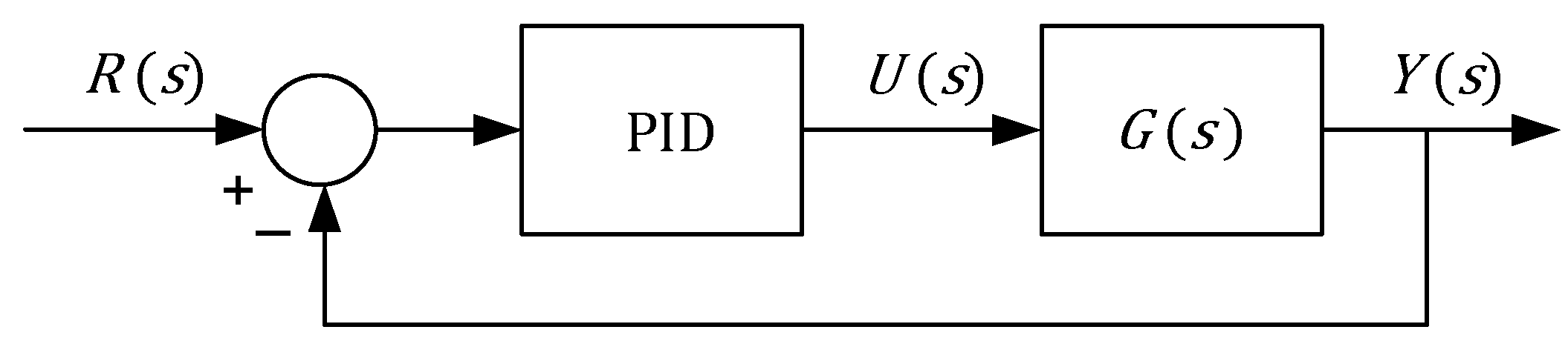
Regarding Laplace’s domains, the corresponding PID transfer functions are:
Feedback control by means of PID is shown in Figure 4. The tuning procedure for a PID controller can be unexpectedly complex. Therefore, besides adaptive and/or heuristic tuning methods via computational algorithms, there are more than a dozen methods based on reaction curves, oscillatory characteristics, and plant model parameters. Among these methods, the most traditional ones are Ziegler–Nichols (Z–N) and Cohen–Coon. Other methods for tuning PID controllers are: Tyreus–Luyben (similar to Z–N in a closed loop), damped oscillation (a 1:4 relation between the first and second overshoot in a closed loop is sought), Chien–Hrones–Reswick, Fertick, Skögestad (based on IMC), Ciancone–Marlin, etc. This work used Tyreus–Luyben and Skögestad [31].
3.2. Gain Scheduling PID Control
The Gain Scheduling control technique is widely used for the control of nonlinear processes. The objective is to identify several operation points in the stationary curve of the process. Then, the adequate parameters of the controller are tuned for each operation point. These parameters will be valid in the corresponding segments of the stationary curve. The set of parameters are introduced into the controller as tables that are read, and optionally interpolated, by the same controller during the process execution. This dynamic change is governed by one or more scheduling variables, which, in general, correspond to the output variables of the process.
Although, theoretically speaking, applying Gain Scheduling to any controller is feasible, a popular and effective method is to combine Gain Scheduling and PID control; hereinafter, GSPID [19,32,33,34,35,36,37,38]. In a traditional PID controller, the Kp, Ki, and Kd gains are invariable for all the operation range, which causes overshoot and oscillations when changing the operation point considered in the first tuning. An effective solution for this problem is to divide the operation range into several segments (in this case, three) and input these gains (obtained from tuning) into a table for each segment. Afterward, the PID controller will change its gains dynamically by reading them from the table, according to the water level.
3.2.1. Division of Level Range into Segments
Considering the type of tank under study, the tank’s volumetric capacity was divided into three segments of approximately 17 cm each: low, medium, and high (see Table 3). After settling the limits of these segments, the operation points for each were located in the middle of each level segment. GSPID tuning was conducted on these operation points.
3.2.2. GSPID Parameter Tuning
A PID controller was tuned for each segment by means of computational simulations and subsequent sharper tuning according to the parameters of the linearized plant in the corresponding operation point . To compare the performance of the GSPID controllers, a classic PID controller was tuned in a fourth operation point, in cm, denominated “nominal point.” Subsequently, through computational simulations, the PID controller gains were searched for in each operation point using the Tyreus–Luyben and Skögestad methods. A lower overshoot, shorter rise time, and less oscillation were preferred, as presented in Table 3.
3.3. IMC Controller
Internal Model Control is a relatively recent control technique, as opposed to traditional control techniques with decades of history such as PID control. Internal Model Control establishes that control can be conducted only if the control system “encapsulates, either implicitly or explicitly, some representation of the process to be controlled” [25,39]. Therefore, the process model in the open loop is embedded in the controller. Regarding other controllers, the IMC type is easier to tune, as the only tuning parameter is the coefficient parameter .
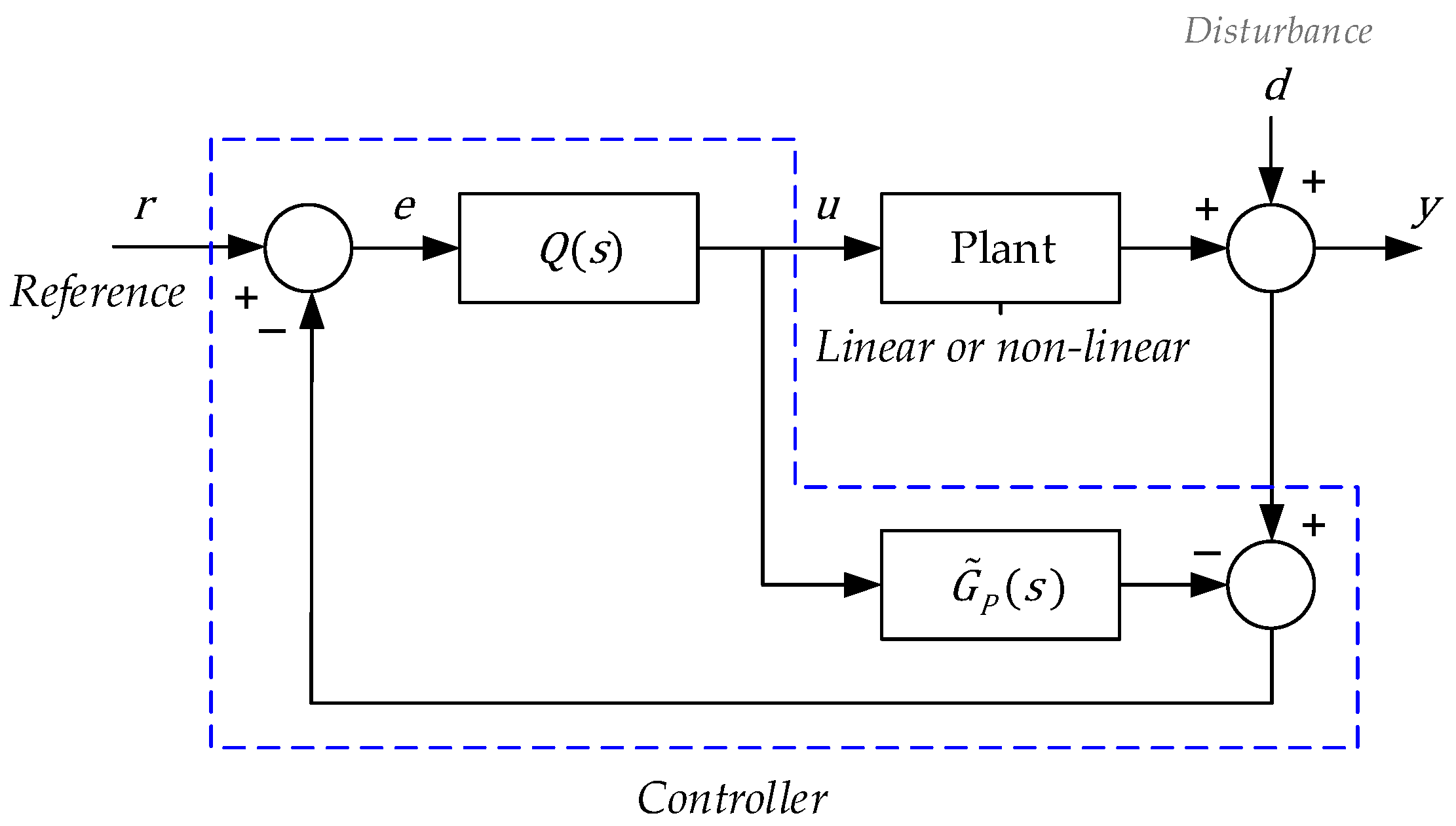
In general, IMC is considered to have good tracking of reference and load changes and good rejection of disturbances. To design an IMC associated with a plant , either linear or nonlinear, a model of the plant is necessary, as shown in Figure 5.
For to be physically achievable, the poles must belong to the left half of the imaginary plane (stability criterion), and the transfer function must be semiproper or proper. For the tank under study, the linearized transfer function at a stationary level , is . For this plant, the function that satisfies the criteria above is:
where corresponds to a first-order filter function, and is the reversible part of the plant model, that is: . With this, we have:
3.4. Fuzzy Logic Control
Fuzzy Logic was originally proposed by Zadeh in 1965. This theory is based on fuzzy sets with degrees of membership ranging between 0 and 1, challenging the traditional set theory. In 1974, Mamdani developed the first fuzzy control applied to a steam engine. The miniaturization and power of digital electronics nowadays allow for the implementation of Fuzzy Logic in compact and reliable controllers. In general, a fuzzy controller consists of the following stages:
- Input fuzzification that assigns degrees of membership to the input membership functions.
- Interaction between the inference engine and a set of linguistic rules, which generates a number of output fuzzy sets.
- Defuzzification of the output set. This generates one or more real numbers (controller outputs) that constitute the control action, whose most used method is the centroid one.
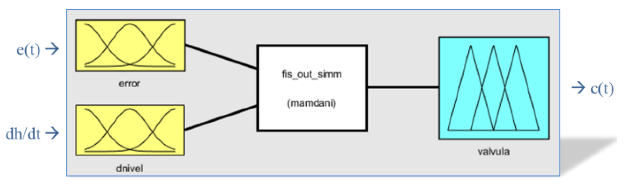
3.4.1. Implementation of Fuzzy Controller in Simulink
The following inputs and output were set for the controller:
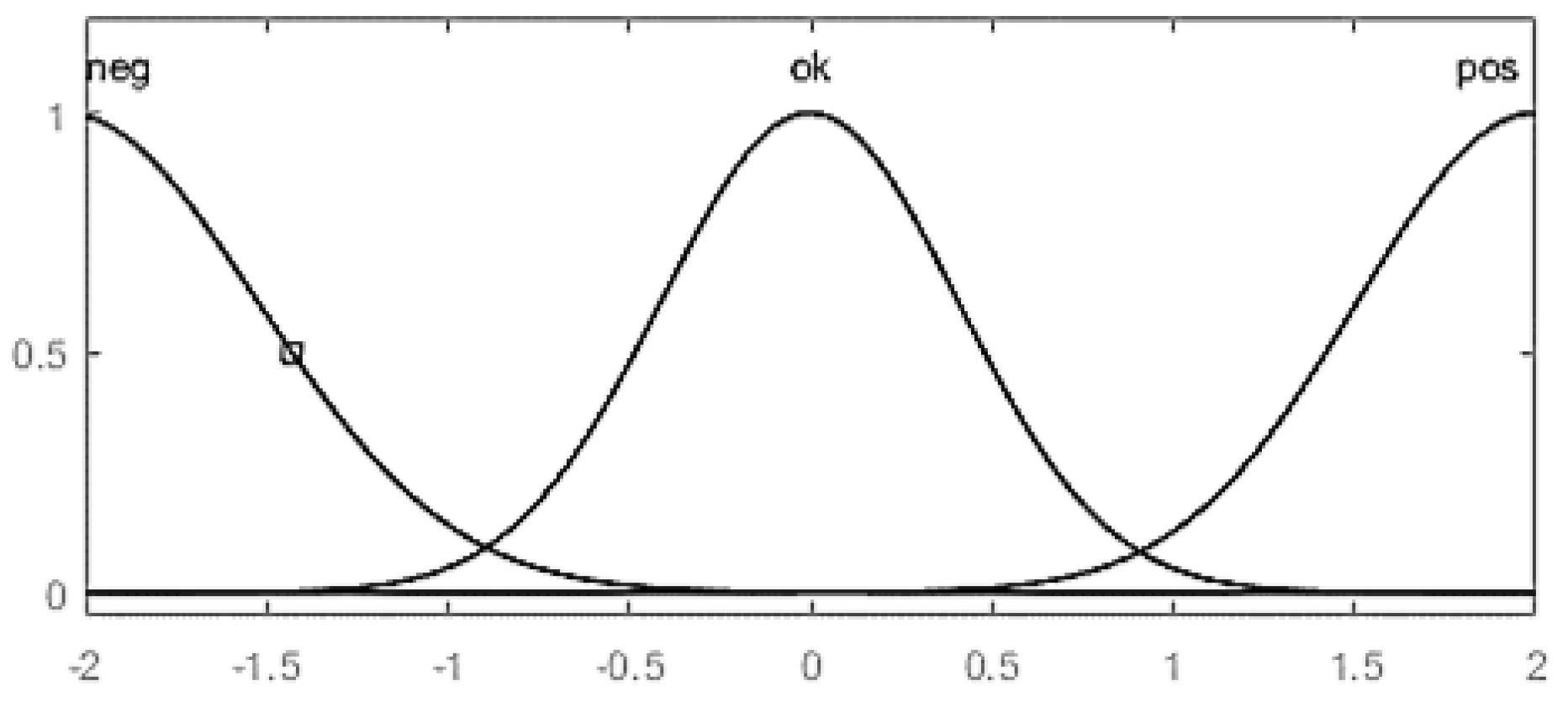
- Input 1: Error, e(t); difference between the reference and the current level of the tank.
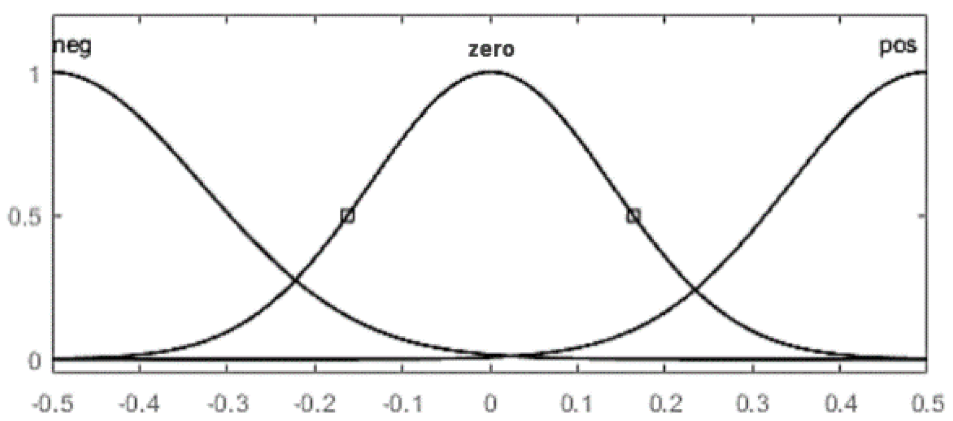
- Input 2: Derivative dh/dt of the tank’s level (the “dnivel” variable), which allows for more precise control of the system by rapid anticipation of changes.
- Output: Relative control action, c(t) (the “valve” output variable), which acts on a modulating valve.
The other characteristics of the designed and simulated fuzzy controller were set as below:
- Fuzzy system: Mamdani
- Logic “Y”: Product
- Logic “O”: Probabilistic
- Defuzzification: Centroid
- Implication: Product
- Aggregation: Maximum
3.4.2. Linguistic Rules of the Controller
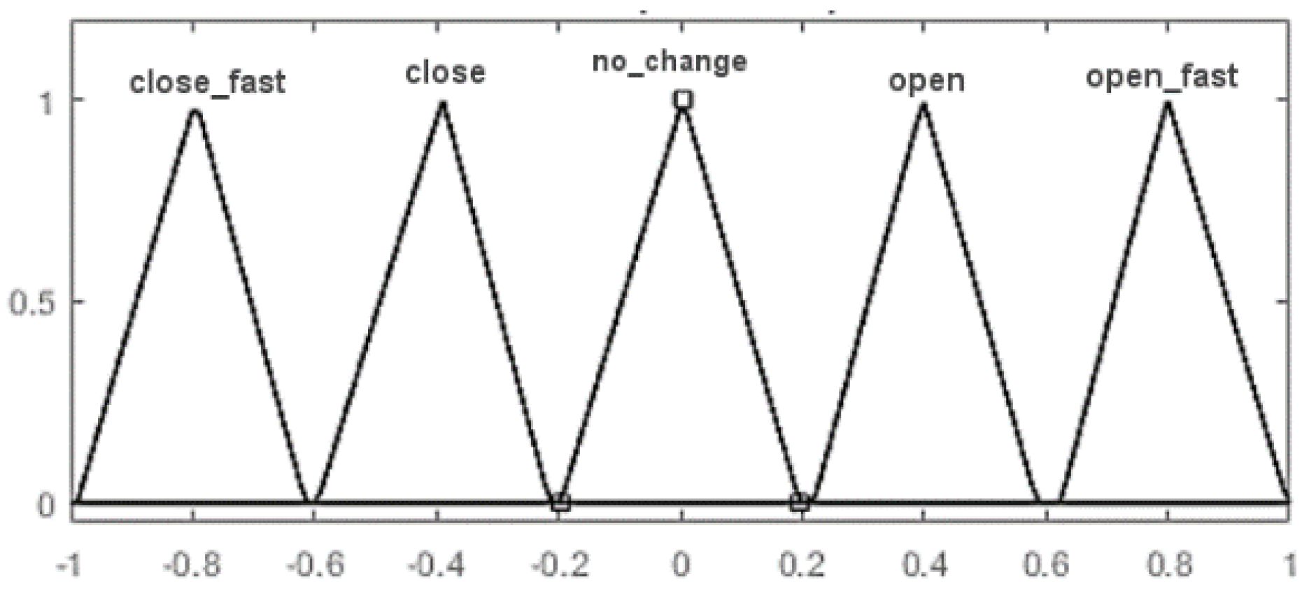
Five rules with unity weights were defined for the five fuzzy output functions as in the following Simulink toolkit syntax:
- If (error is ok) then (valve is no change).
- If (error is neg) then (valve is close fast).
- If (error is pos) then (valve is open fast).
- If (error is ok) and (dnivel is neg) then (valve is open).
- If (error is ok) and (dnivel is pos) then (valve is close).
Regarding these rules, it should be noted that the “fast” control action aims to open or close the simulated valve (by means of the output variable) more than its “nonfast” counterparts.
4. Results Based on Performance Indexes
To assess the performance of the four controllers described above, computational simulations were conducted in parallel, considering identical situations, i.e., the same nonlinear tank, as well as reference changes and disturbances. The following performance indexes were employed [40,41]:
- Integral of the Absolute Error (IAE), defined as:
- Integral of Time-Weighted Absolute Error (ITAE), defined as:
- Integral of the Square Error (ISE), defined as:
- Residual Mean Square (RMS), defined as:
- Residual Standard Deviation (RSD), defined as:
For performance indexes with the integral of error, the incoming signal e(t) of each controller was used. For statistical performance indexes, the reference level and the output level were employed as predicted value sets (pi) and observed value sets (oi), respectively. Additionally, to evaluate the performance of the four controllers more accurately, the following criteria were considered:
- Rising time (considering from 0% to 90% of the reference step’s height).
- Overshoot (% of the reference step’s height).
- Stabilization time (considering a 2% proportional band centered on the desired stationary value).
- Stationary-State Error (% based on the reference level value).
These criteria were organized as parameters in Table 4.
Test scenarios for simulation were the following:
The results of the computational simulations of controller performance in the three test scenarios are detailed below.
4.1. Step at the Reference Level
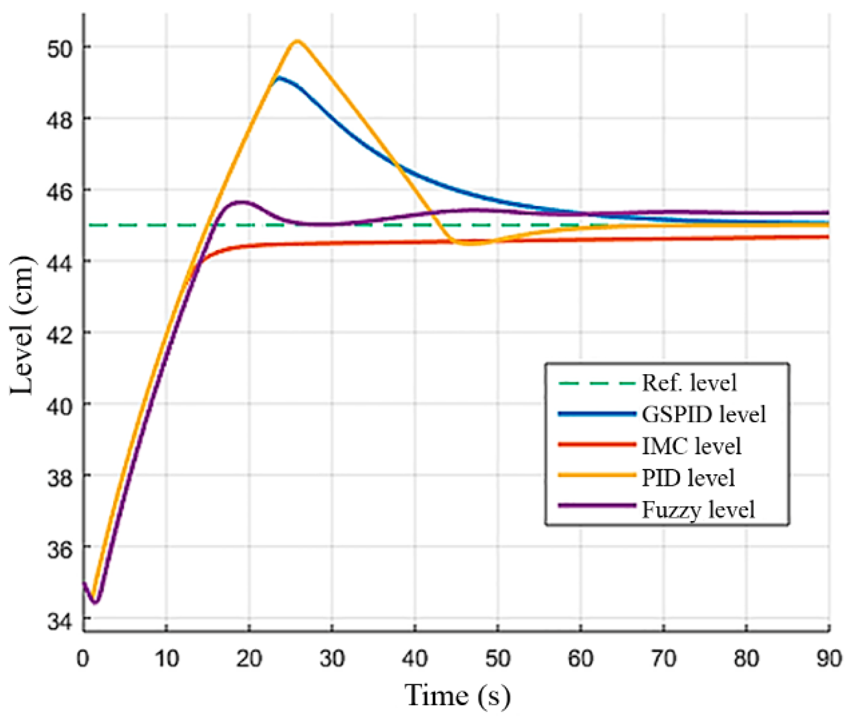
Table 5 contains results based on the tank water level in the stationary state, maximum water level, error, etc., for a 90 s simulation time.
Table 6 presents the results of the performance indexes obtained for the same interval. IMC and fuzzy controllers offer the best performance scores. In addition, overshoot and settling times for these controllers are shorter than those of their PID. In particular, IAE and ITAE indexes tend to punish the high overshoot of PID controllers, with statistical indexes showing clearly a lower dispersion between reference (predicted level) and output (observed level) in IMC and fuzzy controllers. In the 400 s simulations (see Table 7), these controllers exhibit better results in ISE, RMS, and RSD. The slower response of the IMC controller leads to high values in ITAE, while the fuzzy controller delivers a higher IAE index value higher and, noticeably, an ITAE value almost 10 times higher than PID GSPID. This is because the stationary error is below 1%, but not 0, which is amplified in the integral component due to the longer time passed.
It must be noted that, as expected, the ISE, RMS, and RSD values were lower when using IMC and fuzzy control for the two simulation intervals, whereas the values of the IAE and ITAE indexes (especially the latter) increased for the longer time interval. Nonetheless, for this particular test scenario, these two performance indexes did not provide relevant information that allowed us to choose either of them.
The ITAE index and, to a lesser extent, IAE, mistakenly indicate that IMC and fuzzy controllers do not have good performance, which is in contradiction with the graphs obtained, response times, stabilization, low or inexistent overshoot, etc.
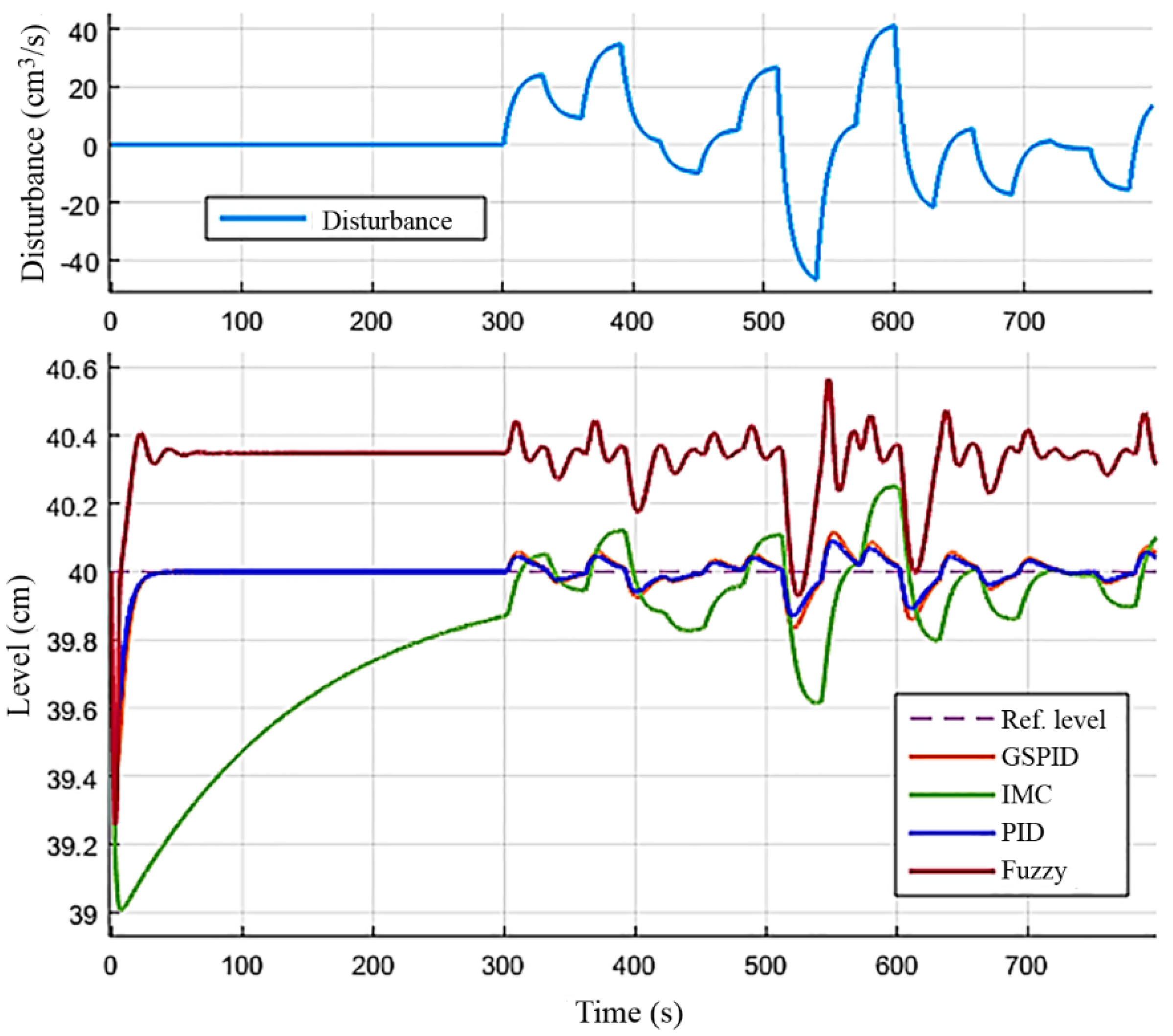
4.2. Random Disturbance on Input Flow
After the first 300 s, a random disturbance is introduced into the tank input flow, representing an unstable flow condition, which is simulated as an arithmetic addition to the input variable in an 800 s computational simulation interval and for a 40 cm level, as shown in Figure 11. As a result, controller performance indexes that delivered the best results are those with PID components, both integrative and statistical, probably due to its integrative component, as shown in Table 8.
From Figure 11, we can conclude that PID controllers are able to handle disturbances with minimum errors in the tank water level. Furthermore, IMC and fuzzy controllers do not perform better than PID.
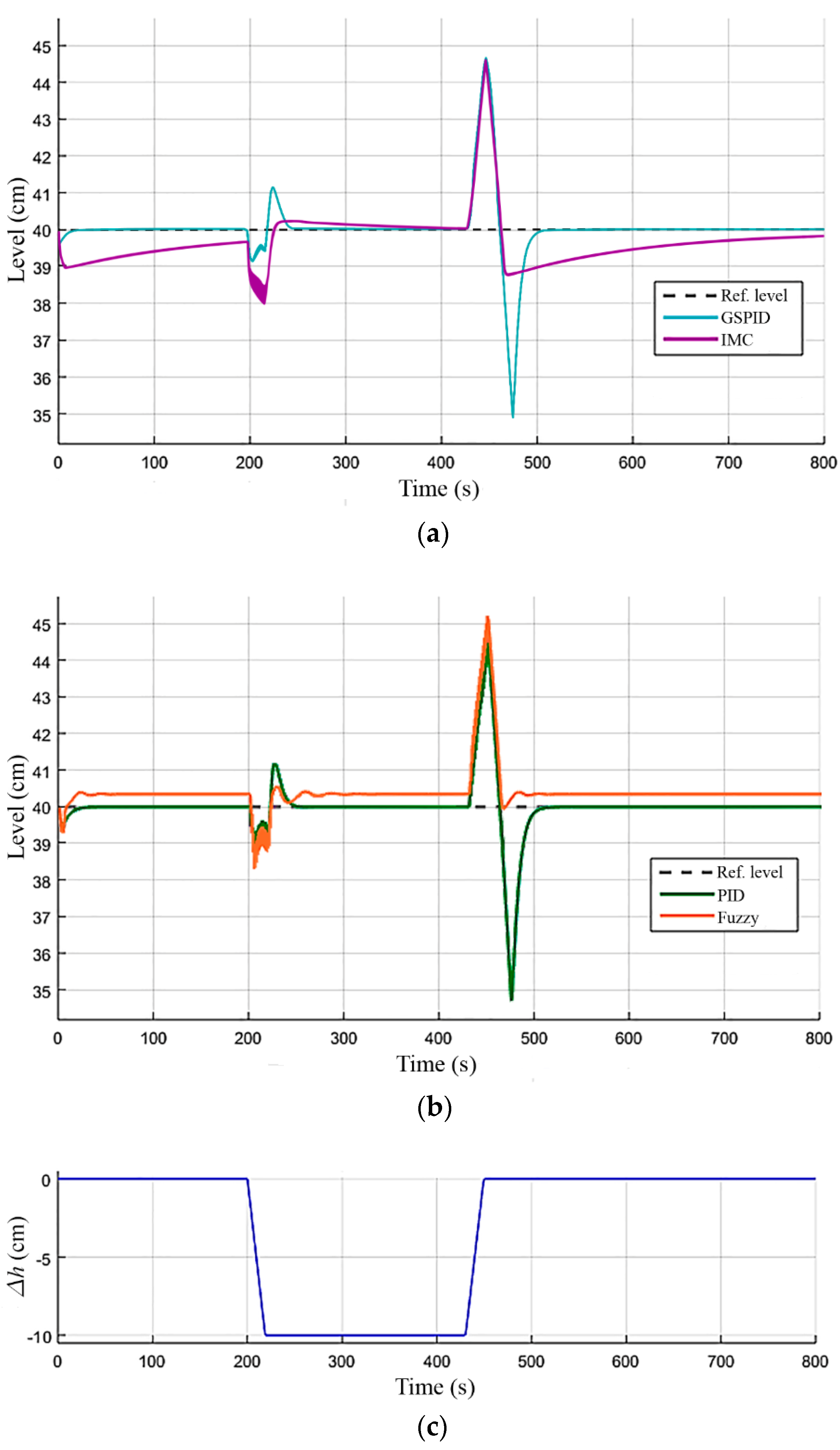
4.3. Transitory Load Disturbance at the Tank Level
This test lasts 800 s and begins with equal initial and reference water levels of 40 cm. Then, a load disturbance is applied between 200 and 450 s, simulated as a lowering of the water level (, as shown in Figure 12. In a real-life scenario, such transitory lowering could be achieved by means of the tank’s auxiliary “L” output. Results are presented in the same figure in order to compare the response of controllers to the disturbance having time as a reference. It is noteworthy that PID and GSPID controllers show an almost identical behavior.
According to Table 9, the fuzzy controller offers the best ISE, RMS, and RSD indexes (by a slim margin). Apparently, IMC would not be a good choice if we compare it to the performance of the PID and GSPID controllers. Nevertheless, the table does not reflect the sudden decrease of PID controllers before 500 s, which is clearly evident in the graph in Figure 12. As expected, controllers with PID components offer the best IAE and ITAE values, confirming once more that these types of indexes are the most suitable for these controllers, as they allow the system input variable to stabilize quickly and make its error tend to zero in the stationary state.
The only time period when none of the controllers reduces overshoot occurs between 430 and 450 s, as the disturbance starts decreasing. In terms of transitory response, at both the beginning of simulation and t = 200 s, the fuzzy controller again shows superiority in performance, with a stationary-state error practically inexistent.
5. Conclusions
In this paper, the water level control of an inverted conical tank system was presented. To determine which of the designed control strategies are the most suitable for an inverted conical tank, a comparative study of the behavior of the system was carried out. With this purpose, and considering situations much closer to reality, a variety of scenarios, such as step responses, random input disturbances, and momentary load disturbances, are conducted.
First, for each applied control strategy, and then, for the measured performance indices, it is concluded that:
PID Control. This controller performs an excellent job in controlling water levels in the vicinity of the operation point for which it was tuned, even tolerating small leaps in the reference, with more than acceptable overshoot and oscillation. Its tendency to eliminate error from the stationary state relatively quickly in comparison with other controllers, as well as its rejection to random disturbances in the input, are definitely strong points in favor of this classic controller. Nonetheless, as evidenced in this study, when attempting to take the level to points farther from the original tuning, excessive overshoot or oscillation appears. These phenomena are compensated for by modern controllers with more efficacy. Moreover, the rejection of load disturbances is not a scenario that favors traditional PID controllers, according to the results of the scenarios researched. Finally, the tuning of a PID controller is challenging and can take many hours of theoretical and practical experiments. Therefore, it can be concluded that this controller is ideal for tanks in which the reference level will not suffer important fluctuations, which will not require retuning, and where there is no possibility of failure in the supply of input flow. As demonstrated in this study, the PID controller compensated for this simulated failure scenario in a satisfactory way.
GSPID. When Gain Scheduling is combined with PID components, it creates PID control, with the advantages already described, along the full operation range of the system. This is achieved through the dynamic commutation/interpolation of gains. The larger the number of segments into which the operation range is divided, the sharper the control over the total system. This partly mitigates excessive overshoot and oscillation, although the natural disadvantages of PID components remain the same. Gain Scheduling offers a huge potential of adaptability to all types of controllers and, in fact, has been successfully used in critical scenarios such as aeronautic control.
IMC. This type of control is relatively recent and has a very interesting conceptual and mathematical approach. Although the need to know the process to be controlled to obtain the internalized model of the controller may be a disadvantage, in practice, the systems to which IMC is applied are well known, and their models have been determined rather accurately. Compared to PID controllers, IMC did not evidence considerable overshooting or oscillation. In addition, the simplicity of its tuning is another point in its favor. Despite its slow response, IMC can be adapted to farther operation points without having to reformulate the internal model. The only significant disadvantages of this controller are its slow response and the single parameter tuning, which, in spite of simplifying the process, impede the controller’s response from adapting to more specific control requirements. In this sense, the PID controller is much more flexible because of its three tunable parameters. Additionally, the capacity of rejecting input flow disturbances is not an outstanding feature in this controller.
Fuzzy control. Results were impressive: low overshoot, minimum oscillation, quick response time for abrupt increases and decreases in the reference, and rapid stabilization in the vicinity of the desired operation point. The only goal that was not achieved with this controller, albeit several attempts, was to eliminate the stationary-state error completely, although this error did not exceed 0.7%. Nonetheless, this result is not considered critical for the tank’s operation. Thus, the fuzzy controller delivers the best results in the scenarios tested in this study.
Performance indexes. The following performance indexes were considered:
- Graphs: as fast visual indicators of the controlled variable behavior.
- Overshoot and times: increase and stabilization.
- Integrative error indexes: IAE, ITAE, ISE.
- Statistical error indexes: RMS, RSD.
In the control of the tank level, excessive overshooting is definitely unwanted, as the content of the tank can leak out. This is a phenomenon that occurs easily when using PID control, and to a lesser extent with GSPID.
PID controllers offer better values in the IAE and ITAE indexes, even with high overshooting. Thus, on their own, these values cannot be taken into account to select the most suitable controller in a specific scenario.
In another vein, controllers that offer better responses than PID, such as IMC and fuzzy controllers, see their performance impaired by these indexes due to their relatively slow response speed (in the case of IMC), or due to stationary-state errors (in the case of fuzzy control). This problem is noticeably heightened in the ITAE index, which calls into question whether these indexes are associated with other controllers different from PID.
The ISE index, and especially the RMS and RSD indexes, allow for a more useful and coherent view of controller performance, as they do not give excessive importance to transitory error or stationary error. When analyzing the tables obtained in this study, it is noticed that these three indexes favor, by a narrow margin, in some cases, controllers without PID components, which is consistent with the graphs obtained and the constraints imposed.
Author Contributions
Conceptualization, C.U. and F.P.; methodology, C.U. and F.P.; software, C.U. and F.P.; validation, C.U. and F.P.; formal analysis, C.U. and F.P.; investigation, C.U. and F.P.; resources, C.U. and F.P.; data curation, C.U. and F.P.; writing—original draft preparation, C.U., and F.P.; writing—review and editing, C.U.; visualization, C.U.; supervision, C.U.; project administration, C.U.; funding acquisition, C.U. All authors have read and agreed to the published version of the manuscript.
Funding
This research received no funding.
Acknowledgments
This work was supported by the Vicerrectoría de Investigación, Desarrollo e Innovación of the University of Santiago of Chile, Chile.
Conflicts of Interest
The authors declare no conflict of interest.
References
- Satpathy, S.; Ramanathan, P. Real Time Control of Non-Linear Conical Tank. Sens. Trans. 2015, 186, 148–153. [Google Scholar]
- Continuous Level Transmitters for Tank Level Measurement. Available online: https://www.gemssensors.com/product/level/continuous-level-transmitters (accessed on 8 April 2021).
- Sabri, L.A.H.; AL-Mshat, H.A. Implementation of Fuzzy and PID Controller to Water Level System using LabView. Int. J. Comput. Appl. 2015, 2015, 116. [Google Scholar]
- Water Tank Level Sensors—Water Level Controls. Available online: https://waterlevelcontrols.com/water-level-sensors-for-water-tanks/ (accessed on 8 April 2021).
- Jondhale, A.; Gaikwad, V.J.; Jondhale, S.R. Level Control of Tank System Using PID Controller—A Review. Int. J. Sci. Res. Dev. 2015, 3, 636–638. [Google Scholar]
- Tank Level Control. Available online: https://www.madisonco.com/tank-level-control (accessed on 8 April 2021).
- Mercy, D.; Girirajkumar, S.M. Design of PSO-PID controller for a nonlinear conical tank process used in chemical industries. ARPN J. Eng. Appl. Sci. 2016, 11, 1147–1153. [Google Scholar]
- Tank or Vessel Level Control Monitoring. Available online: https://sstsensing.com/applications/tank-vessel-level-control-monitoring/ (accessed on 8 April 2021).
- Ullah, I.; Kim, D. An Optimization Scheme for Water Pump Control in Smart Fish Farm with Efficient Energy Consumption. Processes 2018, 6, 65. [Google Scholar] [CrossRef] [Green Version]
- Tank Level Controls and Liquid Level Sensors. Available online: https://www.fluidswitch.com/2016/06/29/tank-level-controls/ (accessed on 8 April 2021).
- Khan, K.A. Simulation of Water Level Control in a Tank Using Fuzzy Logic in Matlab. Int. J. Eng. Comput. Sci. 2017, 6, 56222847. [Google Scholar]
- Liquid Level Controls on Every Process Tank. Available online: https://industrialheatingsystems.com/Liquid-Level-Controls-Process-Tanks.html (accessed on 8 April 2021).
- Kadhim, R.A.; Abdul, A.K.K.; Gitaffa, S.A.H. Implementing of Liquid Tank Level Control Using Arduino-Labview Interfaceing with Ultrasonic Sensor. Kufa J. Eng. 2017, 8, 29–41. [Google Scholar]
- Level Control Applications. Available online: https://www.spiraxsarco.com/learn-about-steam/control-applications/level-control-applications#article-top (accessed on 8 April 2021).
- Karwati, K.; Kustija, J. Prototype of Water Level Control System. IOP Conf. Ser. Mater. Sci. Eng. 2018, 384, 012032. [Google Scholar] [CrossRef] [Green Version]
- Hudedmani, M.G.; Nagaraj, S.N.; Shrikanth, B.J.; Sha, A.A.; Pramod, G. Flexible Automatic Water Level Controller and Indicator. World J. Tech. Eng. Res. 2018, 3, 359–366. [Google Scholar]
- Bagyaveereswaran, V.; Arulmozhivarman, P. Gain Scheduling of a Robust Setpoint Tracking Disturbance Rejection and Aggressiveness Controller for a Nonlinear Process. Processes 2019, 7, 415. [Google Scholar] [CrossRef] [Green Version]
- Zhao, J.; Zhang, X. Inverse Tangent Functional Nonlinear Feedback Control and Its Application to Water Tank Level Control. Processes 2020, 8, 347. [Google Scholar] [CrossRef] [Green Version]
- Jáuregui, C.; Duarte-Mermoud, M.A.; Oróstica, R.; Travieso-Torres, J.C.; Beytía, O. Conical tank level control using fractional order PID controllers: A simulated and experimental study. Cont. Theory Technol. 2016, 14, 369–384. [Google Scholar] [CrossRef]
- Vavilala, S.K.; Thirumavalavan, V.; Chandrasekaran, K. Level control of a conical tank using the fractional order controller. Comput. Electr. Eng. 2020, 87, 106690. [Google Scholar] [CrossRef]
- Keerthana, R.; Babu, K.S.G.; Santhiya, S.; Aravind, P. Level Control of Non Linear Tank Process Using Different Control Technique. Int. J. Adv. Res. Electr. Electron. Instrum. Eng. 2014, 3, 11912–11916. [Google Scholar]
- John, J.A.; Jaffar, N.E.; Francis, R.M. Modelling and Control of Coupled Tank Liquid Level System using Backstepping Method. Int. J. Eng. Res. Tech. 2015, 4, 667–671. [Google Scholar]
- Warier, S.R.; Venkatesh, S. Design of controllers based on MPC for a conical tank system. In Proceedings of the IEEE-International Conference on Advances in Engineering, Science and Management (ICAESM-2012), Nagapattinam, India, 30–31 March 2012; pp. 309–313. [Google Scholar]
- Pushpaveni, T.; Raju, S.S.; Archana, N.; Chandana, M. Modeling and controlling of conical tank system using adaptive controllers and performance comparison with conventional PID. Int. J. Sci. Eng. Res. 2013, 4, 629–635. [Google Scholar]
- Vijula, D.A.; Vivetha, K.; Gandhimathi, K.; Praveena, T. Model based Controller Design for Conical Tank System. Int. J. Comput. Appl. 2014, 85, 8–11. [Google Scholar]
- Wu, D.; Karray, F.; Song, I. Water level control by fuzzy logic and neural networks. In Proceedings of the IEEE Conference on Control Applications, Toronto, ON, Canada, 29–31 August 2005. [Google Scholar]
- Alvisi, S.; Mascellani, G.; Franchini, M.; Bardossy, A. Water level forecasting through fuzzy logic and artificial neural network approaches. Hydrol. Earth Syst. Sci. 2006, 10, 1–17. [Google Scholar] [CrossRef] [Green Version]
- Alvisi, S.; Franchini, M. Fuzzy neural networks for water level and discharge forecasting with uncertainty. Environ. Model. Softw. 2011, 26, 523–537. [Google Scholar] [CrossRef]
- Omijeh, B.O.; Ehikhamenle, M.; Promise, E. Simulated Design of Water Level Control System. Com. Eng. Int. Trans. Syst. 2015, 6, 30–40. [Google Scholar]
- Vijayalakshmi, S.; Manamalli, D.; PalaniKumar, G. Experimental verification of LPV modelling and control for conical tank system. In Proceedings of the 2013 IEEE 8th Conference on Industrial Electronics and Applications (ICIEA), Melbourne, VIC, Australia, 19–21 June 2013; pp. 1539–1543. [Google Scholar]
- Haugen, F. Model-based PID tuning with Skogestad’s method. Model. Identif. Control 2009, 30, 1–7. [Google Scholar]
- Milhim, A.E.; Zhang, Y. Gain Scheduling Based PID Controller for Fault Tolerant Control of a Quad-Rotor UAV. Am. Inst. Aeronaut. Astronaut. 2010, 12, 1–13. [Google Scholar]
- Abdulhamitbilal, E.; Jafarov, E. Gain scheduled automatic flight control systems design for a light commercial helicopter model. WSEAS Trans. Syst. Cont. 2011, 12, 440–455. [Google Scholar]
- Urrea, C.; Kern, J. Fault-Tolerant Controllers in Robotic Manipulators. Performance Evaluations. IEEE Lat. Am. Trans. 2013, 11, 1318–1324. [Google Scholar] [CrossRef]
- Urrea, C.; Venegas, D. Design and Development of Control Systems for an Aircraft. Comparison of Performances through Computational Simulations. IEEE Lat. Am. Trans. 2018, 16, 735–740. [Google Scholar] [CrossRef]
- Urrea, C.; Kern, J. Integrating ROS and IoT in a Virtual Laboratory for Control System Engineering. J. Appl. Math. 2020, 2020, 8987150. [Google Scholar] [CrossRef]
- Gou, L.; Zhidan, L.; Ding, F.; Zheng, H. Aeroengine Robust Gain-Scheduling Control Based on Performance Degradation. IEEE Access 2020, 8, 104857–104869. [Google Scholar] [CrossRef]
- Urrea, C.; Jara, D. Design, Analysis, and Comparison of Control Strategies for an Industrial Robotic Arm Driven by a Multi-Level Inverter. Symmetry 2021, 13, 86. [Google Scholar] [CrossRef]
- Suganthini, P.; Aravind, P.; Girirajkumar, S.M. Design of Model Based Controller for a Non-Linear Process. Int. J. Eng. Appl. Sci. 2014, 3, 3253–3256. [Google Scholar]
- Willmott, C.J.; Ackleson, S.G.; Davis, R.E.; Feddema, J.J.; Klink, K.M.; LeGates, D.R.; O’Donnell, J.; Rowe, C.M. Statistics for the evaluation and comparison of models. J. Geoph. Res. 1985, 90, 8995–9005. [Google Scholar] [CrossRef] [Green Version]
- Urrea, C.; Kern, J.; Alvarado, J. Design and Evaluation of a New Fuzzy Control Algorithm Applied to a Manipulator Robot. Appl. Sci. 2020, 10, 7482. [Google Scholar] [CrossRef]
Figure 1.
Physical diagram of the tank with an auxiliary output L(t).

Figure 2.
Characteristic curve of the stationary state of the tank under study.

Figure 3.
Transfer function in the Laplace that represents the linearized tank in the operation point (,).
Figure 3.
Transfer function in the Laplace that represents the linearized tank in the operation point (,).

Figure 4.
PID controller in a classic closed-loop scheme (Laplace domain).

Figure 5.
Typical block diagram for the IMC controller.

Figure 6.
Fuzzy controller implemented using the Simulink toolkit.

Figure 7.
Membership functions for the input variable “error” e(t).

Figure 8.
Membership functions for the input variable “dnivel” (dh/dt).

Figure 9.
Membership functions for the “valve” output variable.

Figure 10.
Controller’s response to a 35 to 45 cm reference step.

Figure 11.
Random disturbance in the tank input flow (upper graph) and controllers’ response to this disturbance (lower graph).
Figure 11.
Random disturbance in the tank input flow (upper graph) and controllers’ response to this disturbance (lower graph).

Figure 12.
Controllers’ response to a load disturbance at the tank level: (a) GSPID and IMC controllers, (b) PID and Fuzzy controllers; (c) Level change ( as a result of the load disturbance.
Figure 12.
Controllers’ response to a load disturbance at the tank level: (a) GSPID and IMC controllers, (b) PID and Fuzzy controllers; (c) Level change ( as a result of the load disturbance.


Table 1.
Tank parameters.
| Variable | Symbol | Value (cm) |
|---|---|---|
| Maximum radium of the tank | R | 19.25 |
| Minimum radium of the tank | r | 2 |
| Tank height | H | 73 |
| Discharge coefficient | kv | 22 |
Table 2.
Tank model variables.
| Variable | Symbol | Unit |
|---|---|---|
| Input flow (manipulated variable) | Q(t) | (cm3/s) |
| Output flow | Qo(t) | (cm3/s) |
| Water level (controlled variable) | H(t) | (cm) |
| Auxiliary output flow (for load purposes) | L(t) | (cm3/s) |
Table 3.
Level segment parameters for GSPID control and nominal level for PID control.
| Tank | PID Parameters | ||||||
|---|---|---|---|---|---|---|---|
| range (cm) | (cm) | Tuning | |||||
| 10 to 27 | 18.5 | 0.391 | 29.2 | 54.5 | 6.28 | 34.2 | T-L |
| 27 to 44 | 33.5 | 0.541 | 149.1 | 197.7 | 22.5 | 125.5 | T-L |
| 44 to 60 | 52.5 | 0.659 | 396.6 | 301.1 | 18.8 | 200 | SK |
| Nominal level | 40 | 0.575 | 201 | 250 | 28.4 | 158.7 | T-L |
Table 4.
Simulation parameters for reference leap from 35 to 45 cm scenario.
| Initial Reference Level (cm) | Final Reference Level (cm) | Rising Level 90% (cm) | Tolerance Band (%) | Upper Limit, Tol. Band (cm) | Upper Limit, Tol. Band (cm) |
|---|---|---|---|---|---|
| 35 | 45 | 44 | 2.00 | 45.9 | 44.1 |
Table 5.
Results for transitory response and stationary state (s.s.) error, 90 s computational simulation.
Table 5.
Results for transitory response and stationary state (s.s.) error, 90 s computational simulation.
| Controller | S.S. Level (cm) | S.S. Error (%) | Level Max. (cm) | Overshoot (%) | Set Time (s) | Rise Time (s) |
|---|---|---|---|---|---|---|
| GSPID | 45.00 | 0.00 | 49.10 | 41.0 | 46.00 | 13.30 |
| IMC | 44.96 | 0.00 | 44.96 | 0.00 | 15.00 | 14.40 |
| PID | 45.00 | 0.00 | 50.14 | 51.4 | 40.20 | 13.30 |
| Fuzzy | 45.35 | 0.78 | 45.64 | 6.40 | 14.40 | 14.00 |
Table 6.
Performance indexes obtained considering a 90 s simulation time.
| Controller | IAE | ITAE | ISE | RMS | RSD |
|---|---|---|---|---|---|
| GSPID | 159.20 | 3100.00 | 747.10 | 2.9794 | 0.0660 |
| IMC | 110.70 | 1979.00 | 560.20 | 2.6080 | 0.0596 |
| PID | 159.00 | 2801.00 | 821.20 | 3.1147 | 0.0692 |
| Fuzzy | 107.90 | 1665.00 | 647.10 | 2.7819 | 0.0628 |
Table 7.
Performance indexes obtained considering a 400 s simulation time.
| Controller | IAE | ITAE | ISE | RMS | RSD |
|---|---|---|---|---|---|
| GSPID | 159.7 | 3155.0 | 747.1 | 1.4133 | 0.0314 |
| IMC | 153.0 | 10,080.4 | 568.1 | 1.2450 | 0.0279 |
| PID | 159.0 | 2802.0 | 821.2 | 1.4774 | 0.0328 |
| Fuzzy | 215.7 | 27,980.5 | 684.6 | 1.3546 | 0.0300 |
Table 8.
Controller performance indexes for random disturbance in tank input flow.
| Controller | IAE | ITAE | ISE | RMS | RSD |
|---|---|---|---|---|---|
| GSPID | 25.60 | 10,687.10 | 3.710 | 0.0681 | 0.0017 |
| IMC | 179.3 | 39,708.10 | 84.37 | 5.4932 | 0.1380 |
| PID | 20.10 | 8381.000 | 2.310 | 0.0537 | 0.0013 |
| Fuzzy | 265.2 | 10,4710.5 | 93.43 | 0.3416 | 0.0085 |
Table 9.
Controller performance indexes for a load random disturbance at the tank level.
| Controller | IAE | ITAE | ISE | RMS | RSD |
|---|---|---|---|---|---|
| GSPID | 188.4 | 76,245.40 | 505.5 | 0.9491 | 0.0205 |
| IMC | 421.9 | 155,371.5 | 488.4 | 0.9407 | 0.0205 |
| PID | 179.3 | 73,940.40 | 479.3 | 0.9241 | 0.0200 |
| Fuzzy | 369.3 | 150,198.7 | 453.4 | 0.9079 | 0.0195 |
Publisher’s Note: MDPI stays neutral with regard to jurisdictional claims in published maps and institutional affiliations. |
© 2021 by the authors. Licensee MDPI, Basel, Switzerland. This article is an open access article distributed under the terms and conditions of the Creative Commons Attribution (CC BY) license (https://creativecommons.org/licenses/by/4.0/).
Share and Cite
MDPI and ACS Style
Urrea, C.; Páez, F. Design and Comparison of Strategies for Level Control in a Nonlinear Tank. Processes 2021, 9, 735. https://doi.org/10.3390/pr9050735
AMA Style
Urrea C, Páez F. Design and Comparison of Strategies for Level Control in a Nonlinear Tank. Processes. 2021; 9(5):735. https://doi.org/10.3390/pr9050735
Chicago/Turabian StyleUrrea, Claudio, and Felipe Páez. 2021. "Design and Comparison of Strategies for Level Control in a Nonlinear Tank" Processes 9, no. 5: 735. https://doi.org/10.3390/pr9050735
Note that from the first issue of 2016, this journal uses article numbers instead of page numbers. See further details here.