On the Compound Binomial Risk Model with Delayed Claims and Randomized Dividends

Abstract

This paper extends the work of Yuen et al. (2013), who obtained explicit results for the discount-free Gerber–Shiu function for a compound binomial risk model in the presence of delayed claims and a randomized dividend strategy with a zero threshold level. Specifically, we establish a recursion method for computing the Gerber–Shiu expected discounted penalty function, which entails a number of important quantities in ruin theory, within the framework of the compound binomial aggregate claims with delayed by-claims and randomized dividends payable at a non-negative threshold level.

1. Introduction

The compound binomial risk model is a class of discrete-time and discrete-valued risk processes. It was first introduced by Gerber (1988). The model has the form

$$U_t=u+t-{\displaystyle \sum _{i=1}^t}{\xi }_i{X}_i$$

(1)

where $U_t\in \mathbb{Z}=\{\dots ,-2,-1,0,1,2,\dots \}$ is the surplus level at time $t\in {\mathbb{N}}_0=\{0,1,2,\dots \}$ with an initial surplus level $u=U_0\in {\mathbb{N}}_0$; ${\xi }_i$ is a Bernoulli random variable (r.v.) denoting the occurrence of a claim at time i (value 1 indicating a claim); and $X_i$ is the claim size at time i, given a claim occurs then. We note that assuming a unit premium rate in Equation (1) makes it skip-free upwards and simplifies the model greatly. Readers can refer to Avram and Vidmar (2017) for more information. For discrete-time risk models with general premium rates, see, for example, Landriault (2008).

Despite the fact that discrete-time risk models are usually harder to handle than continuous-time models, much research has been done regarding Equation (1) and its variants. Among them, Shiu (1989) and Willmot (1993) investigated the ruin probabilities in the compound binomial model. Dickson (1994) suggested that the compound binomial model is useful in approximating the classical continuous-time compound Poisson model. Cheng et al. (2000) studied various ruin-related quantities in this context. Dos Reis (2004) gave a revision on compound binomial models and studied some interesting new problems regarding the number of claims up to ruin and the number of claims up to recovery. Liu and Zhao (2007) analyzed joint distributions of some actuarial random vectors regarding the model. Moreover, Lefevre and Loisel (2008) investigated the finite-time ruin probabilities for some classical risk models, including the compound binomial model.

It is worth mentioning that compound binomial models are special cases of random walks, which have a long history and still find many useful applications in real life. There are a large number of books and papers in the literature about random walks. Among them, Spitzer (1964) is a good textbook to refer to.

In Yuen and Guo (2001), a type of time-correlation among insurance claims was proposed by introducing the concept of main claims and by-claims. The authors assumed that one main claim (occurring with probability p) would induce a by-claim, which may occur simultaneously with probability $\theta$ or be delayed to the next time period with probability $1-\theta$. The cases of a main claim and its by-claim are summarized in

Table 1. The concept of a by-claim.

	Probability	Current Period	Additional Impact on the Next Period
Case 1	$q=1-p$	No claim	Nil
Case 2	$p\theta$	Main claim and by-claim	Nil
Case 3	$p\left(1-\theta \right)$	Main claim	By-claim

. Main claims and by-claims tend to follow different severity distributions. One can find various relevant examples in real-life insurance practices. For example, multiple lines of insurance claims triggered by the same catastrophic events such as earthquakes or bushfires can be modeled using this correlation structure. Another example arises from the long settlement of certain types of insurance claims. It could take multiple time units to settle claims regarding property damages, bodily injury, and so forth.

Many scholars have done research on this type of dependence structure since then. Wu and Yuen (2004) considered delayed claims in a discrete-time interaction risk model. Yuen et al. (2005) studied the impact of delayed claims on the ultimate ruin probabilities in a compound Poisson risk model. Both Li and Wu (2015) and Xiao and Guo (2007) considered a compound binomial risk model with time-correlated claims. In addition to ruin-related problems, total dividends payable before ruin is another focus point in risk theory. There are many papers in the literature studying risk models with deterministic dividend strategies (constant, linear, etc.). Among them, Wu and Li (2012) studied expected total dividends until ruin in a discrete-time risk model with delayed claims and a constant dividend barrier. Li (2008) analyzed the moments of the present value of the dividends in the compound binomial model under a constant dividend barrier and stochastic interest rates.

Another type of dividend paying strategy is the randomized dividend strategy, under which, when the insurance company’s surplus level is equal to or above a threshold value, dividends are payable with a certain probability. No dividend is payable if the surplus level is below the threshold. Tan and Yang (2006) introduced the concept of the randomized dividend strategy to the compound binomial risk model, followed by Bao (2007) and Landriault (2008). In addition, He and Yang (2010) considered the compound binomial model with randomly paying dividends to shareholders and policyholders. Very recently, Yuen et al. (2017) studied the expected penalty functions for a discrete semi-Markov risk model with randomized dividends.

In this paper, we revisit the compound binomial risk model with the above-mentioned time-correlation and randomized dividends, which has been attempted by Yuen et al. (2013) in a simplified case, that is, a discount-free economic environment with a zero threshold for the randomized dividends. We intend to generalize their work on both aspects, that is, studying the Gerber–Shiu functions with non-zero discount and with a non-negative dividend threshold. The generalization enables us to better relate the risk model under consideration to real-life insurance problems such as the time value of money, and positive dividend thresholds are commonly adopted in practice.

2. The Model

In this paper, we consider the following compound binomial risk model:

$$U_t=u+t-{\displaystyle \sum _{i=1}^t}{\zeta }_i{\mathbf{1}}_{\{U_{i-1}\ge d\}}-{\displaystyle \sum _{i=1}^t}{Z}_i,t\in {\mathbb{N}}_0$$

(2)

where $U_t$ is the surplus level at time t, $u\in {\mathbb{N}}_0$ is the initial surplus, ${\zeta }_i,i\in \mathbb{N}=\{1,2,\dots \}$ are independent and identically distributed (i.i.d.) Bernoulli ($\alpha$) random variables (r.v.’s) denoting the decision on dividends at time i (1 means paying dividends), ${\mathbf{1}}_A$ is an indicator function on event A, $d\in {\mathbb{N}}_0$ is a constant threshold value for the randomized dividend strategy, and $Z_i$ is the total claim amount at time i; $\left\{{\zeta }_i\right\}$ and $\left\{Z_i\right\}$ are independent of each other.

Remark 1.

• $U_t$ is the surplus level after the claims and dividends payable at time t (at the end of period $(t-1,t]$) but before the premiums receivable at time t (at the beginning of period $(t,t+1]$).
• When both dividends and claims are payable at time t, dividends are paid before claims.
• It is worth noting that dividend payments at time i are triggered by two conditions, $U_{i-1}\ge d$ and ${\zeta }_i=1$. No dividend is payable if at least one condition is voided.

Next, we further specify the total claim size $Z_i$ under the time-correlation framework:

$$\begin{array}{lll}{Z}_1\hfill & =& {\xi }_1\left(X_1+{\eta }_1{Y}_1\right)\hfill \\ Z_i\hfill & =& {\xi }_i\left(X_i+{\eta }_i{Y}_i\right)+{\xi }_{i-1}\left(1-{\eta }_{i-1}\right)Y_{i-1},\mathrm{for}i=2,3,\dots \hfill \end{array}$$

where $X_i$ and $Y_i$ denote the main claim amount and by-claim amount at time i, respectively; ${\xi }_i$ is a Bernoulli (p) r.v. with value 1 referring to the occurrence of a main claim at time i; and ${\eta }_i$ is a Bernoulli ($\theta$) r.v. with value 1 denoting the simultaneous occurrence of a by-claim at time i given a main claim occurs at i. If ${\eta }_i=0$, then the by-claim induced at time i will be deferred to time $i+1$. We note that in this model, one by-claim is automated by one main claim with only its timing of payment being random, that is, at the same time as the main claim or one time period later. One example is comprehensive car insurance policies. When a car accident occurs, the total damage to the cars involved in the accident could be the main claim, and bodily injuries caused by the accident could be the associated by-claim. For minor bodily injuries, the diagnoses and treatments should be straightforward, and thus the by-claim occurs simultaneously. However, for severe bodily injuries, the treatment and recovery sometimes could take a long time. This is when the by-claim is delayed. This situation with late/long settlement for certain claims is associated with the incurred-but-not-reported (IBNR) claims in insurance practices, for which the reporting delay is a r.v. Detailed discussions about claims with a random reporting delay can be found in Wüthrich and Merz (2008), Dassios and Zhao (2013), Ahn et al. (2018) and the references therein. In this paper, for the purpose of simplicity, we only consider one time period of delay for by-claims.

We further assume that $X_i$ has the probability function (p.f.) $f_k,k\in \mathbb{N}$ and mean ${\mu }_X$; $Y_i$ has the p.f. $g_k,k\in \mathbb{N}$ and mean ${\mu }_Y$. Additionally, $\left\{X_i\right\},\left\{Y_i\right\}$, $\left\{{\xi }_i\right\}$ and $\left\{{\eta }_i\right\}$, $i\in \mathbb{N}$, are all i.i.d. random sequences and are also independent of each other. They are also independent of $\left\{{\zeta }_i\right\}$. In addition, we denote $X,Y,\eta ,\zeta$ and $\xi$ to be the generic r.v.’s representing the above i.i.d. sequences of r.v.’s.

One can see that Equation (2) can be re-written as, for $t\in \mathbb{N}$,

$$U_t=u+t-{\displaystyle \sum _{i=1}^t}{\zeta }_i{\mathbf{1}}_{\{U_{i-1}\ge d\}}-{\displaystyle \sum _{i=1}^{t-1}}{\xi }_i(X_i+Y_i)-{\xi }_t(X_t+{\eta }_t{Y}_t)$$

(3)

Throughout the rest of this paper, we assume that $0\le \alpha ,\theta \le 1$ and $0<p\le 1$. The positive safety loading condition for Equation (2) takes the form

$$1-\alpha -p({\mu }_X+{\mu }_Y)>0$$

Remark 2.

Some previously considered models in the literature are special cases of Equation (2):

• If $\theta =1$, that is, by-claims always occur simultaneously with their main claims, then it reduces to the model in Tan and Yang (2006).
• If $\alpha =0$, then it reduces to the compound binomial model with time-correlation only; see, for example, Yuen and Guo (2001).
• If both $\theta =1$ and $\alpha =0$, then the model becomes an original compound binomial model.

The main objective in this paper is to study the expected discounted penalty function, also known as the Gerber–Shiu function, in the risk model defined in Equation (2). Because it was first introduced by Gerber and Shiu (1998) in 1998, the Gerber–Shiu function has attracted a great deal of attention in the actuarial science field, and it has been extensively studied under various risk models. Because the function gives us a comprehensive mathematical tool to study ruin-related quantities, it remains one of the popular topics in ruin theory. Recent references on Gerber–Shiu functions include Willmot (2007) and Cheung and Landriault (2010).

For the risk model of Equation (2), we let the r.v. $\tau =min\{t\in \mathbb{N}:U_t<0\}$ be the time of ruin. Then

$$\begin{array}{l}\psi \left(u\right)=\mathbb{P}\{\tau <\infty |U_0=u\},u\in {\mathbb{N}}_0\hfill \end{array}$$

is the ultimate ruin probability. We let $\omega (x,y)$, where $x\in {\mathbb{N}}_0$ and $y\in \mathbb{N}$, be a non-negative penalty function. With a discount factor $v\in (0,1]$, our Gerber–Shiu function has the form

$$m_v(u;d)=\mathbb{E}\left[v^{\tau }\omega \left(U_{\tau -},\left|U_{\tau }\right|\right){\mathbf{1}}_{\{\tau <\infty \}}|U_0=u\right]$$

where the quantity $\omega (U_{\tau -},|U_{\tau }\left|\right)$ can be interpreted as the penalty at the time of ruin for the surplus immediately prior to ruin $U_{\tau -}$ (the surplus before claims payable at $\tau$ but after dividends at $\tau$) and the deficit at ruin $|U_{\tau }|$. Here the dividend threshold d plays a key role in the phenomenon of ruin.

For simplicity, when $v=1$, we would omit the subscript v in $m_v(u;d)$. Thus the discount-free Gerber–Shiu function becomes

$$m(u;d)=\mathbb{E}\left[\omega \left(U_{\tau -},\left|U_{\tau }\right|\right){\mathbf{1}}_{\{\tau <\infty \}}|U_0=u\right]$$

Additionally, when $d=0$, we shall omit d in $m_v(u;d)$ to give $m_v\left(u\right)$. Within the rest of this paper, we investigate $m_v(u;d)$ in the context of Equation (2), extending the results $m\left(u\right)$ obtained in Yuen et al. (2013).

3. Main Results

In this section, we consider the case of $d=0$ and $d>0$ separately.

3.1. The Case of $d=0$.

In this subsection, we focus on $m_v\left(u\right)$. To deal with the time-correlation, we adopt the approach in Yuen and Guo (2001) and define an auxiliary surplus process:

$${\tilde{U}}_t=u+t-{\displaystyle \sum _{i=1}^t}{\zeta }_i{\mathbf{1}}_{\{{\tilde{U}}_{i-1}\ge 0\}}-{\displaystyle \sum _{i=1}^t}{Z}_i-\tilde{Y}{\mathbf{1}}_{\{t\ge 1\}}$$

(4)

where $\tilde{Y}$ is a r.v. with p.f. $g_i,i\in \mathbb{N}$, independent of all the other r.v.’s in the model. The corresponding Gerber–Shiu function is denoted by ${\tilde{m}}_v\left(u\right)$. We note that this auxiliary surplus process refers to the case in which there is a deferred by-claim in the first time period. It enables us to set up a system of equations and to obtain results of $m_v\left(u\right)$.

Before we present our first main result, we introduce the following conditional expected penalty function that enables us to simplify the derivations within the rest of this paper:

$$W_X\left(u\right)=\mathbb{E}\left[\omega (U_{\tau -},|U_{\tau }\left|\right)|\tau <\infty ,U_{\tau -}=u,Z_{\tau }=X\right]$$

where the subscript X indicates the random claim(s) causing ruin. We list some cases of X that are considered thereafter:

• X: one main claim only with p.f. f;
• $X+Y$: one main claim plus its by-claim with p.f. $f\ast g$;
• Y: one by-claim only with p.f. g;
• $X+Y+\tilde{Y}$: one main claim, its by-claim and a delayed by-claim with p.f. $f\ast g^{\ast 2}$;
• $X+\eta Y$: one main claim and an undetermined by-claim with p.f. $\theta (f\ast g)+(1-\theta )f$;
• $\xi (X+\eta Y)+\tilde{Y}$: one delayed by-claim with undetermined main and by-claims with p.f. $qg+p(1-\theta )(f\ast g)+p\theta (f\ast g^{\ast 2})$.

For each case, there is an explicit expression for $W_X\left(u\right)$. For example, for the case of $X+Y$,

$$W_{X+Y}\left(u\right)={\displaystyle \sum _{k=u+1}^{\infty }}\omega \left(u,k-u\right){(f\ast g)}_k$$

For other cases, we just replace $f\ast g$ with its own p.f. in the above expression.

Theorem 1.

Let $\beta =1-\alpha$ and $\widehat{f}\left(z\right)={\sum }_{i=0}^{\infty }{z}^i{f}_i$ be the generating function of f. Similarly, the generating functions of other discrete functions are defined as the symbols with a hat above those functions. When $d=0$, $m_v\left(u\right)$ satisfies the following recursive formula, for $u\in {\mathbb{N}}_0$,

$$\begin{array}{ll}& vq\beta m_v(u+1)\hfill \\ =& (1-vq\alpha )m_v\left(u\right)-v\alpha {\displaystyle \sum _{k=2}^{u+1}}{m}_v(u+1-k)h_k-v\beta {\displaystyle \sum _{k=2}^u}{m}_v(u-k)h_k\hfill \\ & +v^{2}p(1-\theta )\left[{\beta }^2{\displaystyle \sum _{k=2}^{u+2}}{W}_{X+\eta Y}(u+2-k)h_k+2\alpha \beta {\displaystyle \sum _{k=2}^{u+1}}{W}_{X+\eta Y}(u+1-k)h_k\right.\hfill \\ & \left.+{\alpha }^2{\displaystyle \sum _{k=2}^u}{W}_{X+\eta Y}(u-k)h_k\right]-vp[\alpha W_{X+\eta Y}\left(u\right)+\beta W_{X+\eta Y}(u+1)]\hfill \\ & +v^{2}p(1-\theta )\left[{\beta }^2{\displaystyle \sum _{k=2}^{u+2}}{W}_{\xi (X+\eta Y)+\tilde{Y}}(u+2-k)f_k\right.\hfill \\ & \left.+2\alpha \beta {\displaystyle \sum _{k=2}^{u+1}}{W}_{\xi (X+\eta Y)+\tilde{Y}}(u+1-k)f_k+{\alpha }^2{\displaystyle \sum _{k=2}^u}{W}_{\xi (X+\eta Y)+\tilde{Y}}(u-k)f_k\right]\hfill \\ & -v^2\beta (1-\theta )(\alpha h_{u+1}+\beta h_{u+2})[m_v\left(0\right)+p{W}_{X+\eta Y}\left(0\right)]\hfill \\ & +v^{2}p(1-\theta )(\alpha f_{u+1}+\beta f_{u+2})W_{\xi (X+\eta Y)+\tilde{Y}}\left(0\right)\hfill \end{array}$$

(5)

with an initial value

$$\begin{array}{lll}{m}_v\left(0\right)\hfill & =& p\left(1+\frac{\alpha z_0}{\beta }\right){\widehat{W}}_{X+\eta Y}\left(z_0\right)-p{W}_{X+\eta Y}\left(0\right)-\frac{p(1-\theta )(\beta +\alpha z_0)}{\beta A\left(z_0\right)}\widehat{f}\left(z_0\right)\hfill \\ & & \times \left[(\beta +\alpha z_0){\widehat{W}}_{\xi (X+\eta Y)+\tilde{Y}}\left(z_0\right)+W_{\xi (X+\eta Y)+\tilde{Y}}\left(0\right)\right]\hfill \end{array}$$

(6)

where $A\left(z\right)=z-vp(1-\theta )(\beta +\alpha z)\widehat{f}\left(z\right)\widehat{g}\left(z\right)$ and $z_0\in (0,1)$ is the unique solution to the equation $B\left(z\right)=z-v(\beta +\alpha z)(q+p\widehat{f}(z)\widehat{g}(z))=0$.

Proof. 

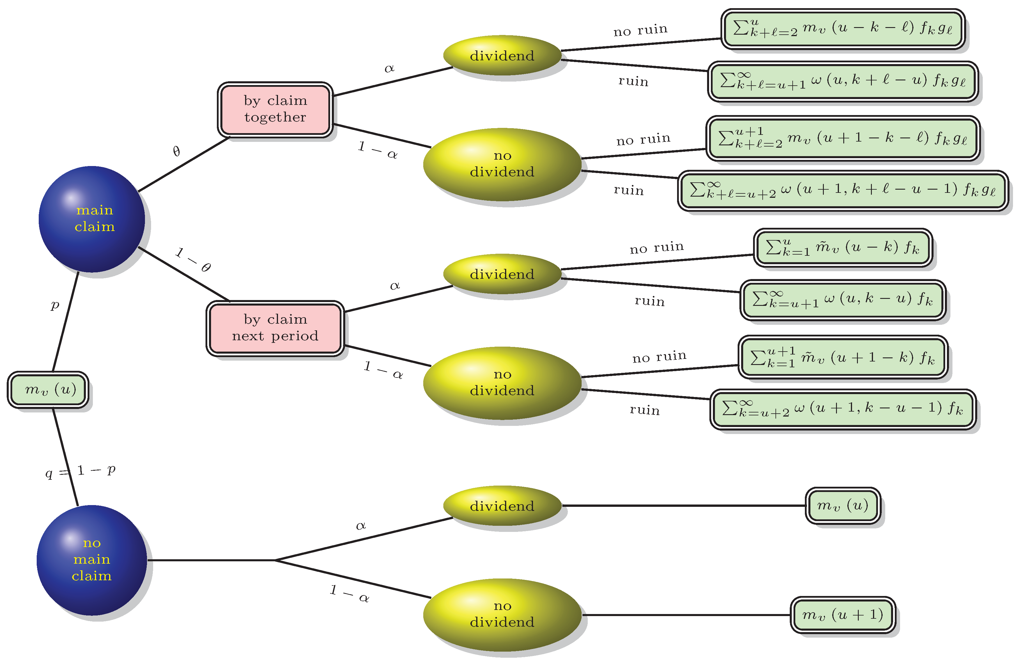
Considering the first time period of Equation (3) with $d=0$, conditional on whether a main claim occurs or not, whether its by-claim is deferred or not, and whether a dividend is payable or not, we list all possible outcomes of the Gerber–Shiu function $m_v\left(u\right)$ at time 1 in Figure 1.

On the basis of Figure 1, we have

$$\begin{array}{lll}& m_v\left(u\right)\hfill & \\ =& vq\beta m_v\left(u+1\right)+vq\alpha m_v\left(u\right)\hfill \\ & +vp\theta \left[\beta {\displaystyle \sum _{k=2}^{u+1}}{m}_v\left(u+1-k\right){(f\ast g)}_k+\alpha {\displaystyle \sum _{k=2}^u}{m}_v\left(u-k\right){(f\ast g)}_k\right]\hfill \\ & +vp\theta \left[\beta {\displaystyle \sum _{k=u+2}^{\infty }}\omega \left(u+1,k-u-1\right){(f\ast g)}_k+\alpha {\displaystyle \sum _{k=u+1}^{\infty }}\omega \left(u,k-u\right){(f\ast g)}_k\right]\hfill \\ & +vp\left(1-\theta \right)\left[\beta {\displaystyle \sum _{k=1}^{u+1}}{\tilde{m}}_v\left(u+1-k\right)f_k+\alpha {\displaystyle \sum _{k=1}^u}{\tilde{m}}_v\left(u-k\right)f_k\right]\hfill \\ & +vp\left(1-\theta \right)\left[\beta {\displaystyle \sum _{k=u+2}^{\infty }}\omega \left(u+1,k-u-1\right)f_k+\alpha {\displaystyle \sum _{k=u+1}^{\infty }}\omega \left(u,k-u\right)f_k\right]\hfill \end{array}$$

(7)

where ${(f\ast g)}_u={\sum }_{i=0}^u{f}_{u-i}{g}_i$ is the convolution of p.f.’s $f_k$ and $g_k$.

Making use of the conditional expected penalty function W defined above, Equation (7) reduces to

$$\begin{array}{ll}& \left(1-vq\alpha \right)m_v\left(u\right)-vq\beta m_v\left(u+1\right)\hfill \\ =& vp\theta \beta {(m_v\ast f\ast g)}_{u+1}+vp\theta \alpha {(m_v\ast f\ast g)}_u+vp\left(1-\theta \right)\beta {({\tilde{m}}_v\ast f)}_{u+1}\\ & +vp\left(1-\theta \right)\alpha {({\tilde{m}}_v\ast f)}_u+vp\beta W_{X+\eta Y}\left(u+1\right)+vp\alpha W_{X+\eta Y}\left(u\right)\hfill \end{array}$$

(8)

Parallel to Equations (7) and (8) and examining the first time period of the auxillary process ${\tilde{U}}_t$, we obtain the following equation of ${\tilde{m}}_v\left(u\right)$:

$$\begin{array}{ll}& {\tilde{m}}_v\left(u\right)\hfill \\ =& vq\beta {\displaystyle \sum _{\ell =1}^{u+1}}{m}_v\left(u+1-\ell \right)g_{\ell }+vq\beta {\displaystyle \sum _{\ell =u+2}^{\infty }}\omega \left(u+1,\ell -u-1\right)g_{\ell }\hfill \\ & +vq\alpha {\displaystyle \sum _{\ell =1}^u}{m}_v\left(u-\ell \right)g_{\ell }+vq\alpha {\displaystyle \sum _{\ell =u+1}^{\infty }}\omega \left(u,\ell -u\right)g_{\ell }\hfill \\ & +vp\theta \left[\beta {\displaystyle \sum _{k=3}^{u+1}}{m}_v\left(u+1-k\right){(f\ast g^{\ast 2})}_k+\alpha {\displaystyle \sum _{k=3}^u}{m}_v\left(u-k\right){(f\ast g^{\ast 2})}_k\right]\hfill \\ & +vp\theta \left[\beta {\displaystyle \sum _{k=u+2}^{\infty }}\omega \left(u+1,k-u-1\right){(f\ast g^{\ast 2})}_k+\alpha {\displaystyle \sum _{k=u+1}^{\infty }}\omega \left(u,k-u\right){(f\ast g^{\ast 2})}_k\right]\hfill \\ & +vp(1-\theta )\left\{\left[\beta {\displaystyle \sum _{k=2}^{u+1}}{\tilde{m}}_v\left(u+1-k\right){(f\ast g)}_k+\alpha {\displaystyle \sum _{k=2}^u}{\tilde{m}}_v\left(u-k\right){(f\ast g)}_k\right]\right.\hfill \\ & \left.+\left[\beta {\displaystyle \sum _{k=u+2}^{\infty }}\omega \left(u+1,k-u-1\right){(f\ast g)}_k+\alpha {\displaystyle \sum _{k=u+1}^{\infty }}\omega \left(u,k-u\right){(f\ast g)}_k\right]\right\}\hfill \\ =& vq\left[\beta {(m_v\ast g)}_{u+1}+\alpha {(m_v\ast g)}_u\right]+vp\theta \left[\beta {(m_v\ast f\ast g^{\ast 2})}_{u+1}+\alpha {(m_v\ast f\ast g^{\ast 2})}_u\right]\hfill \\ & +vp(1-\theta )\left[\beta {({\tilde{m}}_v\ast f\ast g)}_{u+1}+\alpha {({\tilde{m}}_v\ast f\ast g)}_u\right]\hfill \\ & +v\left[\beta W_{\xi (X+\eta Y)+\tilde{Y}}(u+1)+\alpha W_{\xi (X+\eta Y)+\tilde{Y}}\left(u\right)\right]\hfill \end{array}$$

(9)

where $g_x^{\ast 2}={(g\ast g)}_x$ denotes the two-fold convolution of g.

A common result is that the generating function of $f\ast g$ with argument z equals the product of the generating functions of f and g with the same argument; that is, $\widehat{f\ast g}\left(z\right)=\widehat{f}\left(z\right)\widehat{g}\left(z\right)$. With this result, multiplying both sides of Equations (8) and (9) by $z^{u+1}$ and summing over u from 0 to ∞ gives

$$\begin{array}{ll}& \left(1-vq\alpha \right){\displaystyle \sum _{u=0}^{\infty }}{z}^{u+1}{m}_v\left(u\right)-vq\beta {\displaystyle \sum _{u=0}^{\infty }}{z}^{u+1}{m}_v\left(u+1\right)\hfill \\ =& vp\theta \beta {\displaystyle \sum _{u=0}^{\infty }}{z}^{u+1}{(m_v\ast f\ast g)}_{u+1}+vp\theta \alpha {\displaystyle \sum _{u=0}^{\infty }}{z}^{u+1}{(m_v\ast f\ast g)}_u\hfill \\ & +vp\left(1-\theta \right)\beta {\displaystyle \sum _{u=0}^{\infty }}{z}^{u+1}{({\tilde{m}}_v\ast f)}_{u+1}+vp\left(1-\theta \right)\alpha {\displaystyle \sum _{u=0}^{\infty }}{z}^{u+1}{({\tilde{m}}_v\ast f)}_u\hfill \\ & +vp\beta {\displaystyle \sum _{u=0}^{\infty }}{z}^{u+1}{W}_{X+\eta Y}\left(u+1\right)+vp\alpha {\displaystyle \sum _{u=0}^{\infty }}{z}^{u+1}{W}_{X+\eta Y}\left(u\right)\hfill \end{array}$$

and

$$\begin{array}{lll}{\displaystyle \sum _{u=0}^{\infty }}{z}^{u+1}{\tilde{m}}_v\left(u\right)\hfill & =& vq{\displaystyle \sum _{u=0}^{\infty }}{z}^{u+1}\left[\beta {(m_v\ast g)}_{u+1}+\alpha {(m_v\ast g)}_u\right]\hfill \\ & & +vp\theta {\displaystyle \sum _{u=0}^{\infty }}{z}^{u+1}\left[\beta {(m_v\ast f\ast g^{\ast 2})}_{u+1}+\alpha {(m_v\ast f\ast g^{\ast 2})}_u\right]\hfill \\ & & +vp(1-\theta ){\displaystyle \sum _{u=0}^{\infty }}{z}^{u+1}\left[\beta {({\tilde{m}}_v\ast f\ast g)}_{u+1}+\alpha {({\tilde{m}}_v\ast f\ast g)}_u\right]\hfill \\ & & +v{\displaystyle \sum _{u=0}^{\infty }}{z}^{u+1}\left[\beta W_{\xi (X+\eta Y)+\tilde{Y}}(u+1)+\alpha W_{\xi (X+\eta Y)+\tilde{Y}}\left(u\right)\right]\hfill \end{array}$$

The above two equations can be re-written in terms of the generating functions as

$$\begin{array}{ll}& \left[z-v(\beta +\alpha z)(q+p\theta \widehat{f}\left(z\right)\widehat{g}\left(z\right))\right]\widehat{m_v}\left(z\right)\hfill \\ =& vp\left(1-\theta \right)(\beta +\alpha z)\widehat{f}\left(z\right){\widehat{\tilde{m}}}_v\left(z\right)+vp(\beta +\alpha z){\widehat{W}}_{X+\eta Y}\left(z\right)\hfill \\ & -vq\beta m_v\left(0\right)-vp\beta W_{X+\eta Y}\left(0\right)\hfill \end{array}$$

(10)

and

$$\begin{array}{ll}& v(\beta +\alpha z)\widehat{g}\left(z\right)[q+p\theta \widehat{f}\left(z\right)\widehat{g}\left(z\right)]{\widehat{m}}_v\left(z\right)\hfill \\ =& \left[z-vp\left(1-\theta \right)(\beta +\alpha z)\widehat{f}\left(z\right)\widehat{g}\left(z\right)\right]{\widehat{\tilde{m}}}_v\left(z\right)-v(\beta +\alpha z){\widehat{W}}_{\xi (X+\eta Y)+\tilde{Y}}\left(z\right)\hfill \\ & +v\beta W_{\xi (X+\eta Y)+\tilde{Y}}\left(0\right)\hfill \end{array}$$

(11)

Equation (10) $\times \widehat{g}\left(z\right)$ added to Equation (11) yields

$$\begin{array}{lll}{\widehat{\tilde{m}}}_v\left(z\right)\hfill & =& \widehat{g}\left(z\right){\widehat{m}}_v\left(z\right)-\frac{v(\beta +\alpha z)}{z}\left[p{\widehat{W}}_{X+\eta Y}\left(z\right)\widehat{g}\left(z\right)+{\widehat{W}}_{\xi (X+\eta Y)+\tilde{Y}}\left(z\right)\right]\hfill \\ & & +\frac{v\beta }{z}\left[q{m}_v\left(0\right)\widehat{g}\left(z\right)+p{W}_{X+\eta Y}\left(0\right)\widehat{g}\left(z\right)-W_{\xi (X+\eta Y)+\tilde{Y}}\left(0\right)\right]\hfill \end{array}$$

(12)

Substituting Equation (12) into Equation (10) gives

$$\begin{array}{ll}& \left[z-v(\beta +\alpha z)(q+p\widehat{f}\left(z\right)\widehat{g}\left(z\right))\right]{\widehat{m}}_v\left(z\right)\hfill \\ =& vp\left(\alpha +\frac{\beta }{z}\right)A\left(z\right){\widehat{W}}_{X+\eta Y}\left(z\right)-\frac{v^{2}p(1-\theta )}{z}{(\beta +\alpha z)}^2\widehat{f}\left(z\right){\widehat{W}}_{\xi (X+\eta Y)+\tilde{Y}}\left(z\right)\hfill \\ & -\frac{v\beta }{z}A\left(z\right)m_v\left(0\right)-\frac{vp\beta }{z}A\left(z\right)W_{X+\eta Y}\left(0\right)\hfill \\ & -\frac{v^{2}p(1-\theta )}{z}(\beta +\alpha z)\widehat{f}\left(z\right)W_{\xi (X+\eta Y)+\tilde{Y}}\left(0\right)\hfill \end{array}$$

(13)

where $A\left(z\right)=z-vp(1-\theta )(\beta +\alpha z)\widehat{f}\left(z\right)\widehat{g}\left(z\right)$.

Our next task is to find the initial value of $m_v\left(u\right)$, that is, $m_v\left(0\right)$. We let $B\left(z\right)=z-v(\beta +\alpha z)(q+p\widehat{f}\left(z\right)\widehat{g}\left(z\right))$ and $\widehat{h}\left(z\right)=q+p\widehat{f}\left(z\right)\widehat{g}\left(z\right)$, which is the probability generating function (p.g.f.) of $\xi (X+Y)$ (with p.f. denoted by $h_k$, $k\in {\mathbb{N}}_0$). Clearly, $h_0=q,h_1=0$ and $h_k=p{(f\ast g)}_k$ for $k=2,3,\dots$ When $v=1$, as given in Yuen et al. (2013), the fact that $B\left(1\right)=0$ enables us to solve $m_v\left(0\right)$ directly from Equation (13). However, for a general $v\in (0,1]$, we need to use a different approach, that is, making use of the root of equation $B\left(z\right)=0$. One can show that it has a unique positive solution $z_0\in (0,1)$ as follows:

• Firstly, we have $B\left(0\right)=-vq\beta <0$ and $B\left(1\right)=1-v>0$.
• Additionally,

  $$B^{\prime }\left(z\right)=1-v\alpha \widehat{h}\left(z\right)-v(\beta +\alpha z){\widehat{h}}^{\prime }\left(z\right)$$

  which gives $B^{\prime }\left(0\right)=1-v\alpha h_0-v\beta h_1=1-vq\alpha >0$, and for $z\in (0,1]$,

  $$B^{\prime }\left(z\right)\ge 1-v\alpha \widehat{h}\left(1\right)-v{\widehat{h}}^{\prime }\left(1\right)=1-v\alpha -vp({\mu }_x+{\mu }_Y)>0$$

  The last inequality follows from the positive safety loading condition assumed previously.
• Therefore, $B\left(z\right)$ is a strictly increasing function on the interval $(0,1)$ that suffices to prove the existence of a unique solution $z_0\in (0,1)$ to the equation $B\left(z\right)=0$.

Substituting $z=z_0$ into Equation (13) and solving the obtained equation with respect to $m_v\left(0\right)$, we obtain Equation (6).

On the basis of Equations (13) and (6), the recursive formula for $m_v\left(u\right)$ can be established as in Yuen et al. (2013). By comparing coefficients of $z^{u+1}$ on both sides of Equation (13), with some simplifications, we can obtain Equation (5). This completes the proof. ☐

3.2. The Case of $d>0$.

In this subsection, we consider a positive dividend threshold d, $d\in \mathbb{N}$, and the Gerber–Shiu function we consider here is $m_v(u;d)$.

We recall that the surplus process under investigation is

$$U_t=u+t-{\displaystyle \sum _{i=1}^t}{\zeta }_i{\mathbf{1}}_{\left(U_{i-1}\ge d\right)}-{\displaystyle \sum _{i=1}^t}{Z}_i,t\in {\mathbb{N}}_0$$

with an auxiliary surplus process

$${\tilde{U}}_t=u+t-{\displaystyle \sum _{i=1}^t}{\zeta }_i{\mathbf{1}}_{\left\{{\tilde{U}}_{i-1}\ge d\right\}}-{\displaystyle \sum _{i=1}^t}{Z}_i-\tilde{Y}{\mathbf{1}}_{\left\{t\ge 1\right\}}$$

Our second main result is given below:

Theorem 2.

When $d>0$, $m_v(u+1;d)$ satisfies the following recursive formula, for $u\ge d$,

$$\begin{array}{ll}& vq\beta m_v(u+1;d)\hfill \\ =& (1-vq\alpha )m_v(u;d)-v\alpha {\displaystyle \sum _{k=2}^{u+1}}{m}_v(u+1-k;d)h_k-v\beta {\displaystyle \sum _{k=2}^u}{m}_v(u-k;d)h_k\hfill \\ & +v^{2}p(1-\theta )\left[{\beta }^2{\displaystyle \sum _{k=2}^{u+2}}{W}_{X+\eta Y}(u+2-k)h_k+2\alpha \beta {\displaystyle \sum _{k=2}^{u+1}}{W}_{X+\eta Y}(u+1-k)h_k\right.\hfill \\ & \left.+{\alpha }^2{\displaystyle \sum _{k=2}^u}{W}_{X+\eta Y}(u-k)h_k\right]-vp[\alpha W_{X+\eta Y}\left(u\right)+\beta W_{X+\eta Y}(u+1)]\hfill \\ \hfill & +v^{2}p(1-\theta )\left[{\beta }^2{\displaystyle \sum _{k=2}^{u+2}}{W}_{\xi (X+\eta Y)+\tilde{Y}}(u+2-k)f_k\right.\hfill \\ \hfill & \left.+2\alpha \beta {\displaystyle \sum _{k=2}^{u+1}}{W}_{\xi (X+\eta Y)+\tilde{Y}}(u+1-k)f_k+{\alpha }^2{\displaystyle \sum _{k=2}^u}{W}_{\xi (X+\eta Y)+\tilde{Y}}(u-k)f_k\right]\hfill \\ \hfill & -v^2\beta (1-\theta )(\alpha h_{u+1}+\beta h_{u+2})[m_v\left(0\right)+p{W}_{X+\eta Y}\left(0\right)]\hfill \\ \hfill & +v^{2}p(1-\theta )(\alpha f_{u+1}+\beta f_{u+2})W_{\xi (X+\eta Y)+\tilde{Y}}\left(0\right)\hfill \end{array}$$

(14)

where the initial values $m_v(u;d)$, $u=0,1,\dots ,d$, can be determined by solving the following system of $2d+1$ equations, for $u=0,1,\dots ,d-1$:

$$\begin{array}{lll}{m}_v\left(u;d\right)\hfill & =& vq{m}_v\left(u+1;d\right)+vp\theta {\displaystyle \sum _{k=2}^{u+1}}{m}_v\left(u+1-k;d\right){(f\ast g)}_k\hfill \\ & & +vp\left(1-\theta \right){\displaystyle \sum _{k=1}^{u+1}}{\tilde{m}}_v\left(u+1-k;d\right)f_k+vp{W}_{X+\eta Y}(u+1)\hfill \end{array}$$

(15)

$$\begin{array}{lll}{\tilde{m}}_v(u;d)\hfill & =& vq{\displaystyle \sum _{k=1}^{u+1}}{m}_v\left(u+1-k;d\right)g_k+vp\theta \beta {\displaystyle \sum _{k=3}^{u+1}}{m}_v\left(u+1-k;d\right){(f\ast g^{\ast 2})}_k\hfill \\ & & +vp(1-\theta ){\displaystyle \sum _{k=2}^{u+1}}{\tilde{m}}_v\left(u+1-k;d\right){(f\ast g)}_k\hfill \\ & & +v{W}_{\xi (X+\eta Y)+\tilde{Y}}(u+1)\hfill \end{array}$$

(16)

and

$$\begin{array}{lll}{m}_v(d;d)\hfill & =& {\displaystyle \sum _{{\nu }_1=0}^{\infty }}{\displaystyle \sum _{{\nu }_2=1}^d}{\pi }_v({\nu }_1,{\nu }_2)m_v(d-{\nu }_2;d)\hfill \\ & & +{\displaystyle \sum _{{\nu }_1=0}^{\infty }}{\displaystyle \sum _{{\nu }_2=d+1}^{\infty }}{\pi }_v({\nu }_1,{\nu }_2)\omega (d+{\nu }_1;{\nu }_2-d)\hfill \end{array}$$

(17)

We note that the unknown variables in the above system of equations are $m_v(0;d)$, …, $m_v(d;d)$, ${\tilde{m}}_v(0;d)$, …, and ${\tilde{m}}_v(d-1;d)$, and the details of the function ${\pi }_v$ are given in the following proof.

Proof. 

Differently from the derivations in the previous case, our objective functions $m_v(u;d)$ and ${\tilde{m}}_v(u;d)$, $d\in \mathbb{N}$, need to be examined in the following two situations:

• When $u=0,1,\dots ,d-1$, both surplus processes must not pay dividends in the first period.
• When $u=d,d+1,\dots$, the first period may be subject to a dividend payment.

For the case of $u\ge d$, we can proceed similarly to as in Section 3.1:

$$\begin{array}{ll}& m_v\left(u;d\right)\hfill \\ =& vq\beta m_v\left(u+1;d\right)+vq\alpha m_v\left(u;d\right)\hfill \\ & +vp\theta \left[\beta {\displaystyle \sum _{k=2}^{u+1}}{m}_v\left(u+1-k;d\right){(f\ast g)}_k+\alpha {\displaystyle \sum _{k=2}^u}{m}_v\left(u-k;d\right){(f\ast g)}_k\right]\hfill \\ & +vp\left(1-\theta \right)\left[\beta {\displaystyle \sum _{k=1}^{u+1}}{\tilde{m}}_v\left(u+1-k;d\right)f_k+\alpha {\displaystyle \sum _{k=1}^u}{\tilde{m}}_v\left(u-k;d\right)f_k\right]\hfill \\ & +vp\beta W_{X+\eta Y}(u+1)+vp\alpha W_{X+\eta Y}\left(u\right)\hfill \end{array}$$

(18)

and

$$\begin{array}{ll}& {\tilde{m}}_v(u;d)\hfill \\ =& vq\beta {\displaystyle \sum _{\ell =1}^{u+1}}{m}_v\left(u+1-\ell ;d\right)g_{\ell }+vq\alpha {\displaystyle \sum _{\ell =1}^u}{m}_v\left(u-\ell ;d\right)g_{\ell }\hfill \\ & +vp\theta \left[\beta {\displaystyle \sum _{k=3}^{u+1}}{m}_v\left(u+1-k;d\right){(f\ast g^{\ast 2})}_k+\alpha {\displaystyle \sum _{k=3}^u}{m}_v\left(u-k;d\right){(f\ast g^{\ast 2})}_k\right]\hfill \\ & +vp(1-\theta )\left[\beta {\displaystyle \sum _{k=2}^{u+1}}{\tilde{m}}_v\left(u+1-k;d\right){(f\ast g)}_k+\alpha {\displaystyle \sum _{k=2}^u}{\tilde{m}}_v\left(u-k;d\right){(f\ast g)}_k\right]\hfill \\ & +v\left[\beta W_{\xi (X+\eta Y)+\tilde{Y}}(u+1)+\alpha W_{\xi (X+\eta Y)+\tilde{Y}}\left(u\right)\right]\hfill \end{array}$$

(19)

Comparing Equations (18) and (19) with Equations (8) and (9), and making use of the generating function method, we can verify that $m_v(u+1;d)$, $u\ge d$ satisfy the recursive Equation (14), where $m_v(u;d)$, $u=0,1,\dots ,d$ are initial values yet to be determined.

We let $d=0$ and assume a special penalty function:

$$\omega \left(x,y\right)={\mathbf{1}}_{\left\{x={\nu }_1,y={\nu }_2\right\}},x\in {\mathbb{N}}_0,y\in \mathbb{N}$$

where ${\nu }_1\in {\mathbb{N}}_0$ and ${\nu }_2\in \mathbb{N}$ are two constants. Then

$${\pi }_v({\nu }_1,{\nu }_2)=\mathbb{E}\left[v^{\tau }{\mathbf{1}}_{\{U_{\tau -}={\nu }_1,\left|U_{\tau }\right|={\nu }_2\}}{\mathbf{1}}_{\{\tau <\infty \}}|U_0=0\right]$$

(20)

is the discounted joint probability mass function of $U_{\tau -}$ and $|U_{\tau }|$ for ${\nu }_1\in {\mathbb{N}}_0$ and ${\nu }_2\in \mathbb{N}$, when $u=d=0$; or equivalently, it can be interpreted as the discounted joint probability mass function of the surplus level just before the time, at which $U_t$ drops below the dividend threshold level d, and the magnitude of the drop when $u=d\in {\mathbb{N}}_0$. Replacing the penalty function in Equation (6) with ${\mathbf{1}}_{\{x={\nu }_1,y={\nu }_2\}}$ gives, for ${\nu }_2\in \mathbb{N}$,

$$\begin{array}{lll}{\pi }_v(0,{\nu }_2)\hfill & =& \frac{p\alpha z_0}{\beta }\left[\theta {(f\ast g)}_{{\nu }_2}+(1-\theta )f_{{\nu }_2}\right]-\frac{p(1-\theta )(\beta +\alpha z_0)\widehat{f}\left(z_0\right)}{\beta A\left(z_0\right)}\hfill \\ & & \times (1+\beta +\alpha z_0)\left[q{g}_{{\nu }_2}+p(1-\theta ){(f\ast g)}_{{\nu }_2}+p\theta {(f\ast g^{\ast 2})}_{{\nu }_2}\right]\hfill \end{array}$$

(21)

and for ${\nu }_1,{\nu }_2\in \mathbb{N}$,

$$\begin{array}{ll}& {\pi }_v({\nu }_1,{\nu }_2)\hfill \\ =& \frac{p\left(\beta +\alpha z_0\right)z_0^{{\nu }_1}}{\beta }\{\theta {(f\ast g)}_{{\nu }_1+{\nu }_2}+(1-\theta )f_{{\nu }_1+{\nu }_2}-\frac{(1-\theta )(\beta +\alpha z_0)\widehat{f}\left(z_0\right)}{A\left(z_0\right)}\hfill \\ & \times \left[q{g}_{{\nu }_1+{\nu }_2}+p(1-\theta ){(f\ast g)}_{{\nu }_1+{\nu }_2}+p\theta {(f\ast g^{\ast 2})}_{{\nu }_1+{\nu }_2}\right]\}\hfill \end{array}$$

(22)

Both Equations (21) and (22) are used to determine the initial values $m_v(u;d)$, $u=0,1,\dots ,d$.

For the case of $0\le u<d$, there must be no dividend in the first time period certainly; thus this is equivalent to setting $\alpha =0$ in Equations (18) and (19) that gives Equations (15) and (16). Letting $u=0,1,\dots ,d-1$ in Equations (15) and (16) gives us the first $2d$ equations with respect to the $2d+1$ unknown variables $m_v(0;d)$, …, $m_v(d;d)$, ${\tilde{m}}_v(0;d)$, …, and ${\tilde{m}}_v(d-1;d)$. According to the definition and interpretation of ${\pi }_v({\nu }_1,{\nu }_2)$, one can see that $m_v(d;d)$ satisfies Equation (17). Thus, the initial values $m_v(0;d)$, …, $m_v(d;d)$ can be solved. This completes the proof. ☐

4. Final Remarks and Future Work

This paper extended the results given in Yuen et al. (2013) on two aspects, that is, studying the Gerber–Shiu function with a non-zero discount and with a non-negative dividend threshold. We remark that some of the model assumptions adopted in this study are trade-offs between practicability and tractability. On one hand, the compound binomial aggregate claim model and the unity premium level assumption might be criticized because of the lack of generality. On the other hand, the simple nature of these assumptions enables us to tackle the complicated model setup, with main claims and by-claims as well as randomized dividends, all in the same picture.

Additionally, the idea of a randomized dividend strategy might be of limited use in reality. In certain cases, such as mutual funds, the policyholders can be treated as shareholders, and thus the random dividends could be interpreted as a strategic premium reduction depending on the financial status of the insurance company. Additionally, having this possibility examined enables the insurers and regulators to better understand the relationship between ruin-related quantities and dividend strategies and to better manage the risks embedded in the insurance industry.

Some potential future work could be revisiting the main problem of this paper by relaxing some of the key assumptions. One example is to consider the random delay for by-claims; see, for example, Dassios and Zhao (2013). It is worth adopting their approach in the discrete setup, and explicit results are possibly achievable in a similar or simplified way.

References

- Ahn, Soohan, Andrei L. Badescu, Eric C. K. Cheung, and Jeong-Rae Kim. 2018. An IBNR-RBNS insurance risk model with marked Poisson arrivals. Insurance: Mathematics and Economics 79: 26–42. [Google Scholar] [CrossRef]
- Avram, Florin, and Matija Vidmar. 2017. First passage problems for upwards skip-free random walks via the Φ, W, Z paradigm. arXiv, arXiv:1708.06080v1. [Google Scholar]
- Bao, Zhen-hua. 2007. A note on the compound binomial model with randomized dividend strategy. Applied Mathematics and Computation 194: 276–86. [Google Scholar] [CrossRef]
- Cheng, Shixue, Hans U. Gerber, and Elias S. W. Shiu. 2000. Discounted probabilities and ruin theory in the compound binomial model. Insurance: Mathematics and Economics 26: 239–50. [Google Scholar] [CrossRef]
- Cheung, Eric C. K., and David Landriault. 2010. A generalized penalty function with the maximum surplus prior to ruin in a MAP risk model. Insurance: Mathematics and Economics 46: 127–34. [Google Scholar] [CrossRef]
- Dassios, Angelos, and Hongbiao Zhao. 2013. A risk model with delayed claims. Journal of Applied Probability 50: 686–702. [Google Scholar] [CrossRef]
- Dickson, David C. M. 1994. Some comments on the compound binomial model. ASTIN Bulletin 24: 33–45. [Google Scholar] [CrossRef]
- Dos Reis, Alfredo D. Egídio. 2004. The compound binomial model revisited. Paper presented at the 35th International ASTIN Colloquium, Bergen, Norway, June 6–9; Available online: http://www.actuaries.org/ASTIN/Colloquia/Bergen/EgidiodosReis.pdf (accessed on 12 January 2018).
- Gerber, Hans U. 1988. Mathematical fun with the compound binomial process. ASTIN Bulletin 18: 161–68. [Google Scholar] [CrossRef]
- Gerber, Hans U., and Elias S. W. Shiu. 1998. On the time value of ruin. North American Actuarial Journal 2: 48–71. [Google Scholar] [CrossRef]
- He, Lei, and Xiangqun Yang. 2010. The compound binomial model with randomly paying dividends to shareholders and policyholders. Insurance: Mathematics and Economics 46: 443–49. [Google Scholar] [CrossRef]
- Landriault, David. 2008. Randomized dividends in the compound binomial model with a general premium rate. Scandinavian Actuarial Journal 2008: 1–15. [Google Scholar] [CrossRef]
- Lefèvre, Claude, and Stéphane Loisel. 2008. On finite-time ruin probabilities for classical risk models. Scandinavian Actuarial Journal 2008: 41–60. [Google Scholar] [CrossRef]
- Li, Jin-zhu, and Rong Wu. 2015. The Gerber-Shiu discounted penalty function for a compound binomial risk model with by-claims. Acta Mathematicae Applicatae Sinica, English Series 31: 181–90. [Google Scholar] [CrossRef]
- Li, Shuanming. 2008. The moments of the present value of total dividends in the compound binomial model under a constant dividend barrier and stochastic interest rates. Australian Actuarial Journal 14: 175–92. [Google Scholar]
- Liu, Guoxin, and Jinyan Zhao. 2007. Joint distributions of some actuarial random vectors in the compound binomial model. Insurance: Mathematics and Economics 40: 95–103. [Google Scholar] [CrossRef]
- Shiu, Elias S. W. 1989. The probability of eventual ruin in the compound binomial model. ASTIN Bulletin 19: 179–90. [Google Scholar] [CrossRef]
- Spitzer, Frank. 1964. Principles of Random Walk. New York: Springer. [Google Scholar]
- Tan, Jiyang, and Xiangqun Yang. 2006. The compound binomial model with randomized decisions on paying dividends. Insurance: Mathematics and Economics 39: 1–18. [Google Scholar] [CrossRef]
- Willmot, Gordan E. 1993. Ruin probabilities in the compound binomial model. Insurance: Mathematics and Economics 12: 133–42. [Google Scholar] [CrossRef]
- Willmot, Gordan E. 2007. On the discounted penalty function in the renewal risk model with general interclaim times. Insurance: Mathematics and Economics 41: 17–31. [Google Scholar] [CrossRef]
- Wu, Xueyuan, and Shuanming Li. 2012. On a discrete time risk model with time-delayed claims and a constant dividend barrier. Insurance Markets and Companies: Analysis and Actuarial Computations 3: 50–57. [Google Scholar]
- Wu, Xueyuan, and Kam Chuen Yuen. 2004. An interaction risk model with delayed claims. Paper presented at the 35th International ASTIN Colloquium, Bergen, Norway, June 6–9; Available online: http://www.actuaires.org/ASTIN/Colloquia/Bergen/Wu_Yuen.pdf (accessed on 8 September 2015).
- Wüthrich, Mario V., and Michael Merz. 2008. Stochastic Claims Reserving Methods in Insurance. Hoboken: Wiley. [Google Scholar]
- Xiao, Yuntao, and Junyi Guo. 2007. The compound binomial risk model with time-correlated claims. Insurance: Mathematics and Economics 41: 124–33. [Google Scholar] [CrossRef]
- Yuen, Kam Chuen, Mi Chen, and Kam Pui Wat. 2017. On the expected penalty functions in a discrete semi-Markov risk model with randomized dividends. Journal of Computational and Applied Mathematics 311: 239–51. [Google Scholar] [CrossRef]
- Yuen, Kam Chuen, Junyi Guo, and Kai Wang Ng. 2005. On ultimate ruin in a delayed-claims risk model. Journal of Applied Probability 42: 163–74. [Google Scholar] [CrossRef]
- Yuen, Kam Chuen, and Junyi Guo. 2001. Ruin probabilities for time-correlated claims in the compound binomial model. Insurance: Mathematics and Economics 29: 47–57. [Google Scholar] [CrossRef]
- Yuen, Kam Chuen, Jinzhu Li, and Rong Wu. 2013. On a discrete-time risk model with delayed claims and dividends. Risk and Decision Analysis 4: 3–16. [Google Scholar]
Figure 1.
Scenarios of in the first time period.