A Note on Parameter Estimation in the Composite Weibull–Pareto Distribution

Abstract

Composite models have received much attention in the recent actuarial literature to describe heavy-tailed insurance loss data. One of the models that presents a good performance to describe this kind of data is the composite Weibull–Pareto (CWL) distribution. On this note, this distribution is revisited to carry out estimation of parameters via mle and mle2 optimization functions in R. The results are compared with those obtained in a previous paper by using the nlm function, in terms of analytical and graphical methods of model selection. In addition, the consistency of the parameter estimation is examined via a simulation study.

1. Introduction

Composite models have received much attention in the recent actuarial literature to explain unimodal and positively skewed insurance claim datasets (Cooray and Ananda 2005; Scollnik 2007). In one of the recent papers on this topic, Bakar et al. (2015) developed a new approach to derive composite models with the head based on the Weibull distribution to explain heavy-tailed insurance loss data. They proposed models with the tail belonging to a family of transformed beta distributions. One of the models discussed in that paper, the Weibull–Pareto, was previously studied by Cooray (2009) and also by Scollnik and Sun (2012).

Bakar et al. (2015) define the probability density function (PDF) of the latter composite model in the following way:

$$f(x)=\left\{\begin{array}{cc}{\displaystyle \frac{1}{1+\varphi }\frac{f_1(x)}{F_1(\theta )},}& 0<x\le \theta \hfill \\ {\displaystyle \frac{\varphi }{1+\varphi }\frac{f_2(x)}{1-F_2(\theta )}}& \theta <x<\infty .\hfill \end{array}\right.$$

(1)

where $r=\frac{1}{1+\varphi }$ is a mixing weight with $\varphi >0$. Next, these authors took $f_1(x)=\frac{\alpha }{\lambda }{\left(\frac{x}{\lambda }\right)}^{\alpha -1}exp\{-{\left(\frac{x}{\lambda }\right)}^{\alpha }\}$ and $F_1(x)=1-exp\{-{\left(\frac{x}{\lambda }\right)}^{\alpha }\}$ as the PDF and cumulative distribution function (CDF) of the Weibull distribution (with $\alpha ,\lambda >0$) and $f_2(x)=\frac{\beta {\sigma }^{\beta }}{{(\sigma +x)}^{\beta +1}}$ and $F_2(x)=1-{\left(\frac{\sigma }{\sigma +x}\right)}^{\beta }$ as the PDF and CDF of the Pareto type II or Lomax distribution (with $\beta ,\sigma >0$). In this approach, the authors imposed the following conditions: (i) the continuity condition, that is, $f({\theta }^{-})=f({\theta }^{+})$; (ii) the differentiability condition, that is, $f^{\prime }({\theta }^{-})=f^{\prime }({\theta }^{+})$; (iii) in order to have a genuine density, the mixing weights must sum to 1 with $\varphi =-\frac{\frac{d}{d\theta }log{F}_1(\theta )}{\frac{d}{d\theta }log(1-F_2(\theta ))}$; (iv) the threshold $\theta$ is expressed as a function of the other parameters, and it is obtained by solving $\frac{d}{d\theta }log\frac{f_1(\theta )}{f_2(\theta )}=0$. Clearly, conditions (i) and (ii) are satisfied, as they are imposed in the third composite Weibull–Pareto (CWL) model in Scollnik and Sun (2012); it is simple to see that condition (iii) implies that $\varphi =\frac{f_1(\theta )(1-F_2(\theta ))}{f_2(\theta )F_1(\theta )}$, and therefore $r=\frac{f_2(\theta )F_1(\theta )}{f_2(\theta )F_1(\theta )+f_1(\theta )(1-F_2(\theta ))}$; this result coincides with Equation (4.5) in Scollnik and Sun (2012) by taking $r\frac{f_1(\theta )}{F_1(\theta )}=(1-r)\frac{f_2(\theta )}{1-F_2(\theta )}$; finally, condition (iv) is equivalent to the condition $\frac{f_1^{\prime }(\theta )}{f_1(\theta )}=\frac{f_2^{\prime }(\theta )}{f_2(\theta )}$, which is satisfied by the third CWL model in Scollnik and Sun (2012).

This model was fitted by Scollnik and Sun (2012) and Bakar et al. (2015) to a dataset that consisted of 2492 fire losses, adjusted for inflation, arising from claims in Copenhagen. It was recorded in millions of Danish krone (DKK) for a period from 1980 to 1990. This dataset can be found in the SMPracticals add-on package for R, available from the CRAN website http://cran.r-project.org/. Bakar et al. (2015) also fitted this model to a second dataset that concerned general liability claims. They examined the allocated loss adjustment expenses (ALAE) in thousands of US$. The dataset comprised 1500 general liability claims randomly chosen from late settlement lags. This dataset can be found in the R evd add-on package. In Bakar et al. (2015), the nlm optimization function in R was used to fit different composite models, on the basis of the Weibull distribution, to these datasets. This function is included in the stats package. Although this method can be faster than other algorithms in terms of the number of iterations to converge, its main limitation is that it only uses a Newton-type algorithm. This algorithm is more sensitive to the shape of the likelihood surface, and its application depends to a great extent on the type of data available. Consequently, it might lead to a false solution. On this note, we fit these two datasets by using the mle (stats4 package) and mle2 (bbmle package) optimization functions. These functions rely on Nelder-Mead, quasi-Newton and conjugate-gradient algorithms. We show that the fit of the CWL distribution to the latter dataset by using the R optimization functions mle and mle2 considerably differs from that reported in Table 2 in Bakar et al. (2015) in terms of three measures of model selection. Moreover, it is illustrated that the fit in terms of these two optimization functions adheres much closer to the empirical data in the respect of a Zipf plot. These plots (see Levy 2009) use a double logarithmic framework to explain the relationship between the city log-rank and city log-size. In this work, the graphs have been adapted to show the connection between the claim log-rank and claim log-size.

The rest of this paper is organized as follows. In Section 2, parameter estimation for the ALAE dataset has been computed for the CWL distribution using two different optimization functions in R, the mle and mle2 optimization functions. The results are compared with the estimates obtained in Bakar et al. (2015) by using the nlm optimization function in terms of analytical and graphical methods of model validation. Next, in Section 3, a simulation analysis has been performed for the estimates obtained in the previous section under the two optimization functions considered in this work. Finally, conclusions are given in the last section.

2. Parameter Estimation and Model Selection

The Weibull distribution (W), Pareto type II or Lomax distribution (L) and the CWL distribution have been firstly fitted to Danish fire insurance losses using the functions mle and mle2 in R. The results coincide with those reported in Table 1 in Scollnik and Sun (2012) and in Table 2 in Bakar et al. (2015), obtained using the nlm optimization function in R. For the CWL model, the estimated value for the threshold $\theta$ was 0.9717. The corresponding standard error was 0.0069. The value of the unrestricted mixing weight r was 0.1075. However, for the CWL model, with respect to the ALAE dataset, the estimates, the negative of the maximum of the log-likelihood function (NLL), Akaike’s information criterion (AIC) and Schwarz’s Bayesian criterion (SBC) differed considerably from the values reported in Table 1 in Bakar et al. (2015). They are shown below (

Table 1. R optimization function, parameter estimates, standard errors (S.E.), Akaike’s information criterion (AIC) and Schwarz’s Bayesian criterion (SBC) under composite Weibull–Pareto (CWL) distribution model for allocated loss adjustment expenses (ALAE) dataset.

Model	R Function	Estimate (S.E.)	NLL	AIC	SBC
Weibull Lomax	mle	$\widehat{\alpha }=1.0375(0.0386)$	5047.110	10,102.220	10,123.473
		$\widehat{\lambda }=6.3207(0.4898)$
		$\widehat{\sigma }=9.5937(2.2659)$
		$\widehat{\theta }=8.0407(2.0436)$
Weibull Lomax	mle2	$\widehat{\alpha }=1.0375(0.0386)$	5047.110	10,102.220	10,123.473
		$\widehat{\lambda }=6.3207(0.4892)$
		$\widehat{\sigma }=9.5937(2.2646)$
		$\widehat{\theta }=8.0407(2.0407)$

).

Under both optimization functions, the estimated value for the shape parameter $\beta$ was 1.8386, and the value of the unrestricted mixing weight r was 0.6216. Of course, as the global maximum of the likelihood surface is not guaranteed, different initial values were considered as seed points. It is observable that the performance of the CWL model does not improve the behaviour of the Pareto type II distribution by taking SBC as the criterion of comparison (the value obtained was 10,118.258).

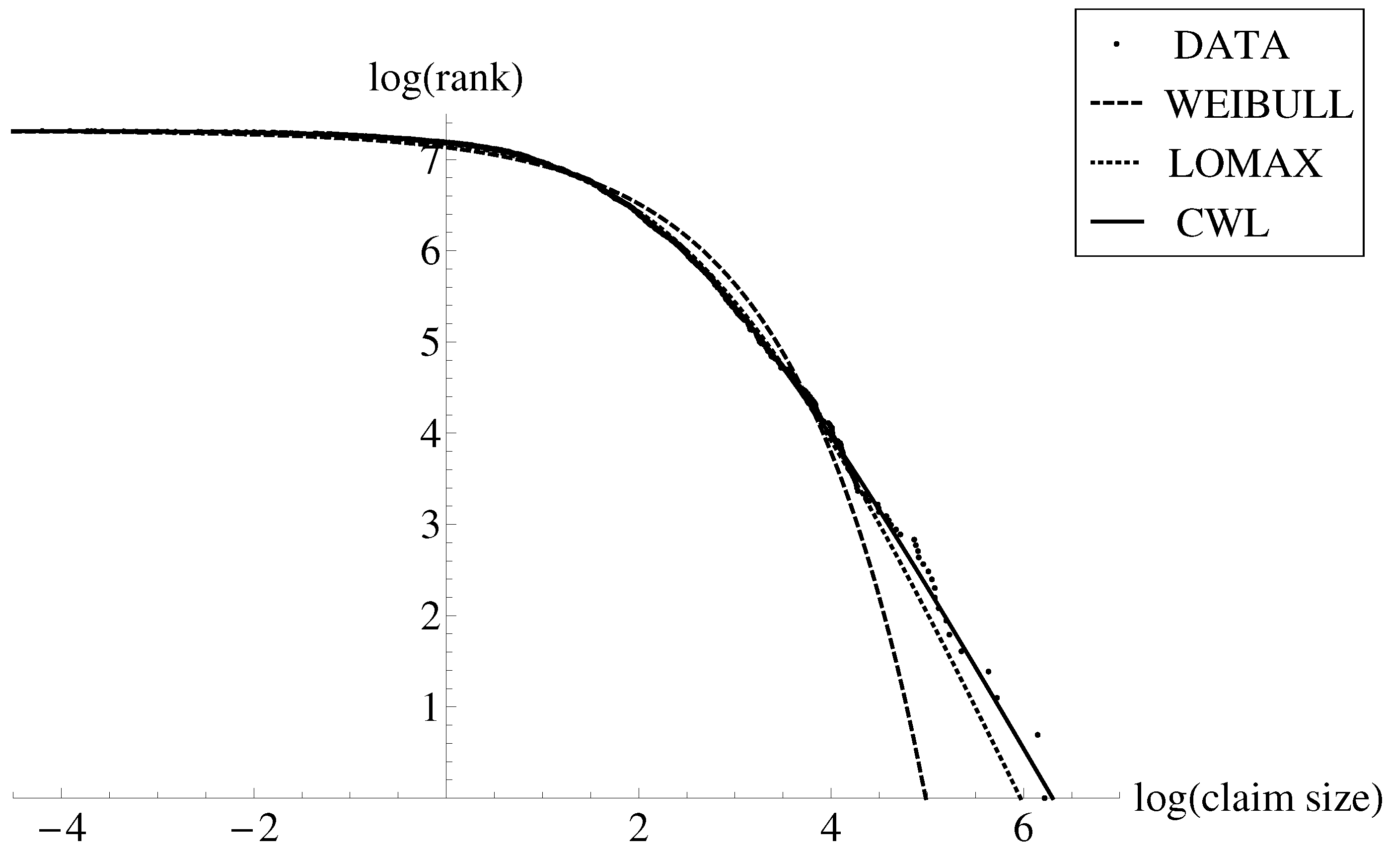
These results largely differed from those reported in Table 1 in Bakar et al. (2015) using the nlm optimization function. For those results, the estimated threshold $\theta$ was 750.958, and the unrestricted mixing weight r was 0.0694. In addition to this, by combining the latter values together with the results in Table 1 in that paper, the figures of the NLL, AIC and SBC were 536,438.272, 1,072,876.544 and 1,072,905.797, respectively. In Figure 1 is illustrated the relationship between the claim log-rank and claim log-size. The scatter dots represent the empirical data. For example, the largest claim, 501.863, is represented as the dot on the bottom right; it is ranked number 1, $log(\mathrm{rank})=0$, and it has a logarithm of claim size of $log(\mathrm{size})=6.218$. On the other hand, the lowest claim 0.015, is depicted as the dot in the top left; it is ranked number 1500, $log(\mathrm{rank})=7.313$, and it has a logarithm of claim size of $log(\mathrm{size})=-4.200$. We have superimposed to this graphical representation the graphs of the inverse of the survival function of the Weibull (W, dashed), Pareto type II or Lomax (L, dotted) and CWL (CWL, solid) distributions. The inverse of the survival function of the latter model is given by

$$S^{-1}(u)=\left\{\begin{array}{cc}{\displaystyle F_1^{-1}\left(\frac{F_1(\theta )}{r}(1-u)\right),}& 0<u\le r\hfill \\ {\displaystyle F_2^{-1}\left((1-F_2(\theta ))\frac{1-r-u}{1-r}\right),}& r<u<1\hfill \end{array}\right.$$

(2)

where $u\in (0,1)$ and $F_1^{-1}(·)$ and $F_2^{-1}(·)$ are the quantile functions of the Weibull and Lomax distributions, respectively. It is observable that the Weibull distribution (although it explains the low part of the distribution) fails to describe either the moderate-size claims or large claims. The Pareto type II distribution is a good model to explain this dataset; however, it underestimates the largest claims. On the other hand, the CWL model remains closer to the empirical data than the other two standard distributions throughout the whole set of empirical points. In addition, the largest observations are better explained by means of this composite model.

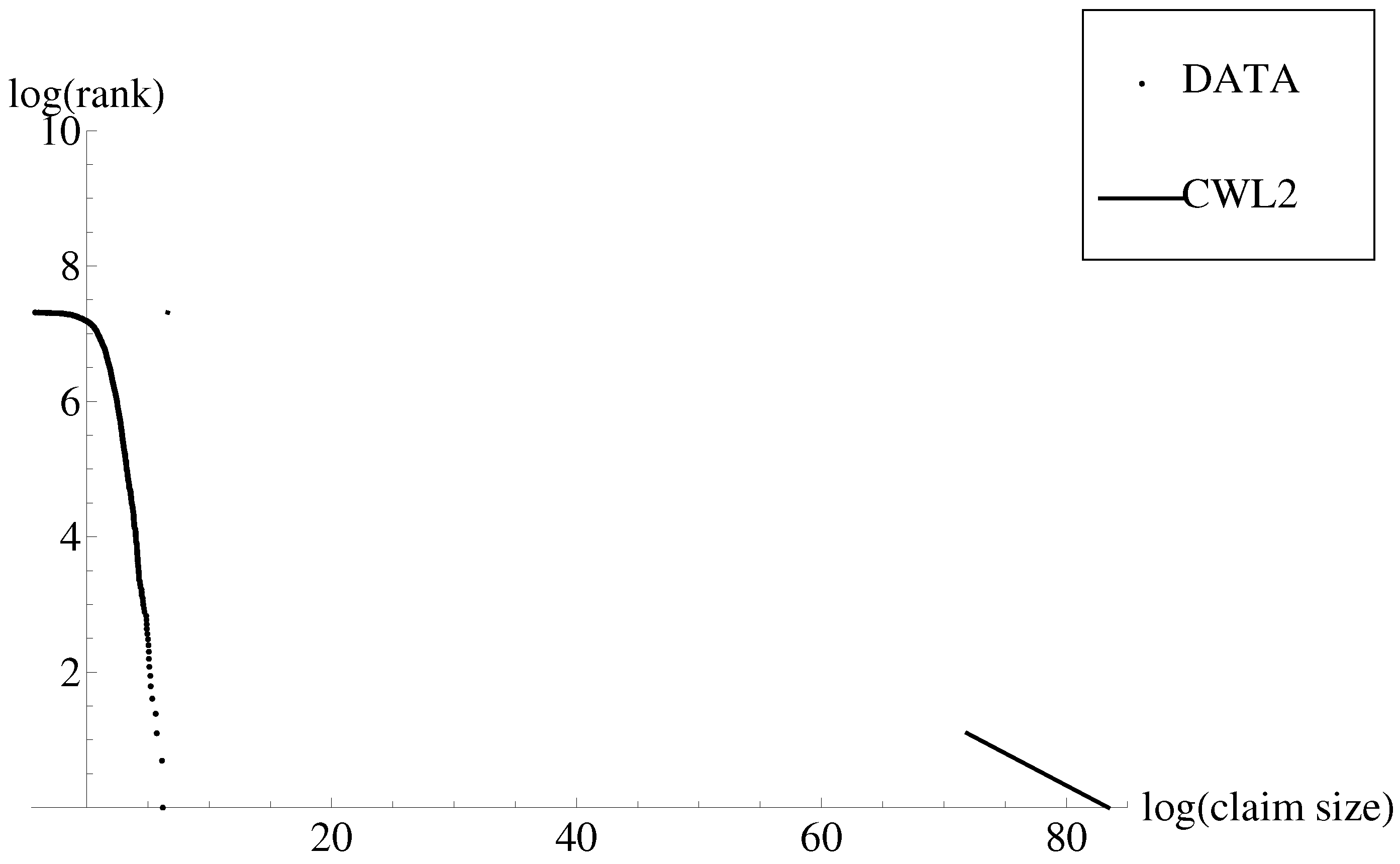
In Figure 2 is shown the relationship between the claim log-rank and claim log-size. Again, the scatter dots represent the empirical data. The inverse of the survival function of the CWL model under the parameter estimates in Table 1 in Bakar et al. (2015) (CWL2) has been superimposed to this scatterplot. It is noticeable that first, the quantile function of the first component (i.e., Weibull) cannot be derived for all the values of $0<u\le r$, and the quantile function of the second component (i.e., Lomax) lies far away from the empirical data.

The empirical values at risk (VaRs) at the 99% security level for the Danish fire insurance losses and for the ALAE dataset were 24.61 and 131.71, respectively. The corresponding values under the CWL model were 22.648 and 117.523. Similarly, the empirical conditional tail expectations (CTE) for the Danish fire insurance losses and for the ALAE dataset were 54.60 and 222.68, respectively. On the other hand, the VaR and CTE values reported in Table 3 in Bakar et al. (2015) for the CWL model were 58.079 and 268.913. The latter values also differed from those reported above.

3. A Simulation Analysis

Asymptotic normality of the maximum likelihood estimates holds only under certain regularity conditions that are not easy to check analytically. In this section, the performance of the maximum likelihood estimates with respect to the sample size is assessed. This assessment is on the basis of simulations. We show that the usual asymptotic results still hold for composite distributions.

A general form to generate a random variate x from the CWL distribution is based on the use of the inverse transformation method of simulation, as the CDF of the CWL distribution is invertible. If u is a value generated from the uniform distribution $U(0,1)$, then a value generated from Equation (1) can be obtained as follows:

• If $u\le r$, then

  $$x=\lambda {\left\{-log\left[1-\frac{u}{r}\left(1-exp\left[-{\left(\frac{\theta }{\lambda }\right)}^{\alpha }\right]\right)\right]\right\}}^{1/\alpha }$$
• If $u>r$, then

  $$x=(\sigma +\theta ){\left(\frac{1-u}{1-r}\right)}^{-1/\beta }-\sigma$$

We used the estimates reported in Table 1 to perform a simulation analysis. Because of the highly skewed nature of the original dataset, and given that the sample size of this dataset was 1500, we allowed the sample size to vary from 1000 to 2000 in steps of 500. The simulation study was carried out 1000 times. We denote ${\widehat{\mathsf{\Theta }}}_i=({\widehat{\alpha }}_i,{\widehat{\lambda }}_i,{\widehat{\sigma }}_i,{\widehat{\theta }}_i)$ and $s_{{\widehat{\mathsf{\Theta }}}_i}=(s_{{\widehat{\alpha }}_i},s_{{\widehat{\lambda }}_i},s_{{\widehat{\sigma }}_i}{s}_{{\widehat{\theta }}_i})$ for $i=1,2,\cdots ,1000$. We have calculated the following measures:

• Average bias of the simulated estimates:

  $$A{B}_n(\widehat{\mathsf{\Theta }})=\frac{1}{N}\sum _{i=1}^N({\widehat{\mathsf{\Theta }}}_i-\mathsf{\Theta })\mathrm{for}\mathsf{\Theta }=(\widehat{\alpha },\widehat{\lambda },\widehat{\sigma },\widehat{\theta })$$
• Average root-mean-square errors:

  $$RMS{E}_n(\widehat{\mathsf{\Theta }})=\sqrt{\frac{1}{N}\sum _{i=1}^N{({\widehat{\mathsf{\Theta }}}_i-\mathsf{\Theta })}^2}\mathrm{for}\mathsf{\Theta }=(\widehat{\alpha },\widehat{\lambda },\widehat{\sigma },\widehat{\theta })$$
• Coverage probability: percentage of confidence intervals containing the true value of $\mathsf{\Theta }$ at the 95% confidence level.

Table 2. Average bias (AB) for the composite Weibull–Pareto (CWL) distribution model involving 1000 simulations of samples of size n for the mle (second column) and mle2 (third column) functions.

	R Function
Sample Size $\mathit{n}$	mle	mle2
$n=1000$	$AB(\widehat{\alpha })=0.0194$	$AB(\widehat{\alpha })=0.0318$
	$AB(\widehat{\lambda })=-0.2747$	$AB(\widehat{\lambda })=-0.4641$
	$AB(\widehat{\sigma })=-0.1697$	$AB(\widehat{\sigma })=-0.3226$
	$AB(\widehat{\theta })=0.0174$	$AB(\widehat{\theta })=0.0532$
$n=1500$	$AB(\widehat{\alpha })=0.0105$	$AB(\widehat{\alpha })=0.0127$
	$AB(\widehat{\lambda })=-0.1800$	$AB(\widehat{\lambda })=-0.1710$
	$AB(\widehat{\sigma })=0.0374$	$AB(\widehat{\sigma })=-0.2408$
	$AB(\widehat{\theta })=-0.0653$	$AB(\widehat{\theta })=0.1194$
$n=2000$	$AB(\widehat{\alpha })=0.0078$	$AB(\widehat{\alpha })=0.0059$
	$AB(\widehat{\lambda })=-0.1177$	$AB(\widehat{\lambda })=-0.1070$
	$AB(\widehat{\sigma })=-0.0909$	$AB(\widehat{\sigma })=-0.2437$
	$AB(\widehat{\theta })=0.0350$	$AB(\widehat{\theta })=0.1371$

shows that the average bias was always positive for $\widehat{\alpha }$ under the two optimization functions and always decreased with the sample size n. The values of the parameters $\widehat{\lambda }$ and $\widehat{\sigma }$ were always positive. We note that there existed some discrepancy in the values between the two functions.

Table 3. Average root-mean-square errors (RMSE) for the composite Weibull–Pareto (CWL) model involving 1000 simulations of samples of size n for the mle function (second column) and mle2 function (third column).

	R Function
Sample Size $\mathit{n}$	mle	mle2
$n=1000$	$RMSE(\widehat{\alpha })=0.0763$	$RMSE(\widehat{\alpha })=0.0957$
	$RMSE(\widehat{\lambda })=1.1908$	$RMSE(\widehat{\lambda })=1.5083$
	$RMSE(\widehat{\sigma })=3.5354$	$RMSE(\widehat{\sigma })=4.4062$
	$RMSE(\widehat{\theta })=3.8563$	$RMSE(\widehat{\theta })=3.7280$
$n=1500$	$RMSE(\widehat{\alpha })=0.0557$	$RMSE(\widehat{\alpha })=0.0588$
	$RMSE(\widehat{\lambda })=0.9361$	$RMSE(\widehat{\lambda })=0.9129$
	$RMSE(\widehat{\sigma })=2.7904$	$RMSE(\widehat{\sigma })=2.8334$
	$RMSE(\widehat{\theta })=3.1370$	$RMSE(\widehat{\theta })=3.2292$
$n=2000$	$RMSE(\widehat{\alpha })=0.0459$	$RMSE(\widehat{\alpha })=0.0437$
	$RMSE(\widehat{\lambda })=0.7717$	$RMSE(\widehat{\lambda })=0.7283$
	$RMSE(\widehat{\sigma })=2.3913$	$RMSE(\widehat{\sigma })=2.4617$
	$RMSE(\widehat{\theta })=2.7425$	$RMSE(\widehat{\theta })=2.7723$

shows the average root-mean-square error. These values consistently reduced with the sample size, regardless of the optimization function used. The values obtained for this composite model also highlight the consistency of the parameter estimation. In general, a reasonably large sample size is needed to produce a good interval estimation for the parameter.

Table 4. Average coverage probability (CP) at the 95% confidence level for the composite Weibull–Pareto (CWL) model involving 1000 simulations of samples of size n for the mle (second column) and mle2 (third column) functions.

	R Function
Sample Size $\mathit{n}$	mle	mle2
$n=1000$	$CP(\widehat{\alpha })=0.9220$	$CP(\widehat{\alpha })=0.9170$
	$CP(\widehat{\lambda })=0.8720$	$CP(\widehat{\lambda })=0.8690$
	$CP(\widehat{\sigma })=0.9050$	$CP(\widehat{\sigma })=0.9050$
	$CP(\widehat{\theta })=0.8270$	$CP(\widehat{\theta })=0.8330$
$n=1500$	$CP(\widehat{\alpha })=0.9420$	$CP(\widehat{\alpha })=0.9150$
	$CP(\widehat{\lambda })=0.8980$	$CP(\widehat{\lambda })=0.8880$
	$CP(\widehat{\sigma })=0.9100$	$CP(\widehat{\sigma })=0.9220$
	$CP(\widehat{\theta })=0.8580$	$CP(\widehat{\theta })=0.8590$
$n=2000$	$CP(\widehat{\alpha })=0.9310$	$CP(\widehat{\alpha })=0.9310$
	$CP(\widehat{\lambda })=0.8970$	$CP(\widehat{\lambda })=0.9020$
	$CP(\widehat{\sigma })=0.9190$	$CP(\widehat{\sigma })=0.9210$
	$CP(\widehat{\theta })=0.8830$	$CP(\widehat{\theta })=0.8860$

illustrates that the coverage probabilities were closer to the intended significance confidence level of 0.95 for the estimate $\widehat{\alpha }$ than for the other parameter estimates. It is evident that by increasing the sample size, the accuracy of the parameter estimates increases. Of course, the true parameter values are those previously given in Table 1, and these were the limits of the estimates as the sample size n increased.

4. Conclusions

In this paper, the parameter estimation and model assessment of the CWL distribution have been revisited. It has been shown that the formulation of this model in Bakar et al. (2015) is equivalent to the third CWL model in Scollnik and Sun (2012). The two datasets examined in Bakar et al. (2015) have been fitted to data by using the optimization functions mle and mle2 in R. In spite of the fit to Danish fire insurance losses, the dataset coincides with that reported in Table 1 in Scollnik and Sun (2012) and in Table 2 in Bakar et al. (2015) (under nlm function); the fit to the ALAE dataset considerably differs from that reported in Table 1 in the latter paper in terms of the three measures of model selection. These results are also confirmed in terms of a Zipf plot. The consistency of these estimates was examined via a simulation analysis. However, no matter which method was used to find the maximum likelihood estimates of the parameters, these estimates were biased. Alternatively, we could have followed the work of Giles et al. (2013). In that paper, the authors carried out an exploration of the bias of the maximum likelihood estimators of the Lomax distribution parameters. They also completed a comparison with alternative methods of reducing the bias when the sample size was relatively small. As an extension of this work, this study could be implemented for the CWL distribution. This investigation could be complemented with the alternative bias-correction mechanism based on Efron’s bootstrap resampling as in Wang and Wang (2017). These authors derived simple closed-form expressions for the second-order biases of the maximum likelihood estimators of the weighted Lindley distribution parameters.

Although the performance of composite models is, in general, better than the behaviour of standard distributions to describe highly skewed loss data or city size data (see Calderín-Ojeda 2016), the practitioner must be cautious when choosing these models, as the principle of parsimony (Klugman et al. 2008) can be violated. This principle states that unless there is considerable evidence to choose otherwise, a simple model is preferred. In this sense, for the ALAE dataset, the superiority of composite Weibull models to describe highly skewed data is arguable. In this regard, the behaviour of the Weibull–Pareto model is worse than that of the Lomax distribution in terms of SBC. The fit to data of the latter model would have been even better if we had considered the shifted Lomax distribution with PDF $f(x)=\frac{\beta {(\sigma +\theta )}^{\beta }}{{(\sigma +x)}^{\beta +1}},x>\theta ,\sigma >-\theta$ where $\theta =0.015$ (e.g., minimum sample value). In this case, we obtained 5048.502, 10,101.004 and 10,111.631 for the NLL, AIC and SBC, respectively. Consequently, the best choice of a model always depends on the set of data being analyzed, and therefore, it requires an exercise in judgment and experience.

References

- Abu Bakar, Shaiful Anuar, Nor Aishah Hamzah, Mastoureh Maghsoudi, and Saralees Nadarajah. 2015. Modeling loss data using composite models. Insurance: Mathematics and Economics 61: 146–54. [Google Scholar]
- Calderín-Ojeda, Enrique. 2016. The distribution of all French communes: A composite parametric approach. Physica A: Statistical Mechanics and its Applications 450: 385–94. [Google Scholar]
- Cooray, Kahadawala. 2009. The Weibull-Pareto composite family with applications to the analysis of unimodal failure rate data. Communications in Statistics—Theory and Methods 38: 1901–15. [Google Scholar]
- Cooray, Kahadawala, and Malwane M. A. Ananda. 2005. Modeling actuarial data with a composite Lognormal-Pareto model. Scandinavian Actuarial Journal 5: 321–34. [Google Scholar]
- Giles, David E., Hui Feng, and Ryan T. Godwin. 2013. On the bias of the maximum likelihood estimator for the two-parameter Lomax distribution. Communications in Statistics—Theory and Methods 42: 1934–50. [Google Scholar]
- Klugman, Stuart A., Harry H. Panjer, and Gordon E. Willmot. 2008. Loss Models: From Data to Decisions, 3rd ed. Hoboken: John Wiley. [Google Scholar]
- Levy, Moshe. 2009. Gibrat’s Law for (all) cities: Comment. American Economic Review 99: 1672–75. [Google Scholar]
- Scollnik, David P. M. 2007. On composite Lognormal-Pareto models. Scandinavian Actuarial Journal 1: 20–33. [Google Scholar]
- Scollnik, David P. M., and Chenchen Sun. 2012. Modeling with Weibull-Pareto models. North American Actuarial Journal 16: 260–72. [Google Scholar]
- Wang, Min, and Wentao Wang. 2017. Bias-corrected maximum likelihood estimation of the parameters of the weighted Lindley distribution. Communications in Statistics—Theory and Methods 46: 530–45. [Google Scholar]
Figure 1.
Relationship between claim rank and claim size in log–log scale and graphs of the inverse of the survival function of Weibull (W, dashed), Lomax (L, dotted) and composite Weibull–Pareto (CWL, solid) distributions.
Figure 2.
Relationship between claim rank and claim size in log–log scale and graphs of the inverse of the survival function of composite Weibull–Pareto model in Bakar et al. (2015) (CWL2, solid).