Variation of Individual Location Radiance in VIIRS DNB Monthly Composite Images

Abstract

With the growing size and use of night light time series from the Visible Infrared Imaging Radiometer Suite Day/Night Band (DNB), it is important to understand the stability of the dataset. All satellites observe differences in pixel values during repeat observations. In the case of night light data, these changes can be due to both environmental effects and changes in light emission. Here we examine the stability of individual locations of particular large scale light sources (e.g., airports and prisons) in the monthly composites of DNB data from April 2012 to September 2017. The radiances for individual pixels of most large light emitters are approximately normally distributed, with a standard deviation of typically 15–20% of the mean. Greenhouses and flares, however, are not stable sources. We observe geospatial autocorrelation in the monthly variations for nearby sites, while the correlation for sites separated by large distances is small. This suggests that local factors contribute most to the variation in the pixel radiances and furthermore that averaging radiances over large areas will reduce the total variation. A better understanding of the causes of temporal variation would improve the sensitivity of DNB to lighting changes.

1. Introduction

The starting point of every observation of the Earth system by satellite remote sensing is a measurement of radiance. This is true regardless of whether the application is in meteorology, geoscience, urban studies, or even just astronaut photographs taken in order to share the pleasure of viewing Earth from space. The radiance observed in the visible band during daytime depends critically on the reflectance properties of the surface and the solar and viewing angles, and to a lesser extent on atmospheric factors. Considerable work has been devoted over more than half a century to understanding how and why daytime radiances vary, in order to make it possible to extract remotely sensed observables (e.g., vegetation phenology) from the datasets.

In stark contrast to the daytime situation, regular repeated observations of Earth’s artificial light emissions at night with a calibrated radiometer began only in 2012. (The Defense Meteorological Satellite Program Operational Linescan System instrument that produced the well known first global maps of night light emissions [1] was not radiance calibrated. The gain of the sensor was frequently changed for operational reasons, and these changes were not recorded.) Instead of reflectance and solar angle, the most critical factors affecting observations of nighttime radiance in brightly lit areas are the details of the artificial light sources in the area of interest, and the presence or absence of screening in the satellite’s viewing direction. Now that a radiometrically calibrated instrument is available, it is possible to address the question “how stable are observations of Earth’s sources of artificial light?” for the first time.

This question is important, because remote sensing applications using visible band data taken at night are frequently focused on analyzing changes in artificial light. For example, night light data have been used to monitor changes in urban footprints [2], gross domestic product [3], and infrastructure damage due to war [4,5,6]. Changes in both spatial positions and intensities of emitted visible light over time are of interest to those studying light pollution, for example to examine light encroachment into protected areas [7,8], light emission from individual bright sources [9], as well as global and national rates of change [10]. Moreover, individual night light datasets are often fused with other geospatial datasets to provide information at subnational levels [11,12,13]. To what extent are such analyses observing real changes in light, as opposed to variations due to other factors?

There are a number of factors that cause repeat observations of an identical location to have different radiances. Specifically for the case of satellite observations with large spatial areas imaged in each pixel (e.g., the Day/Night Band on the Visible Infrared Imaging Radiometer Suite Instrument), these include the following:

• differences in imaging angle [14,15];
• the time of night (because lights turn off as night progresses) [16,17];
• seasonal variations in vegetation and snow cover [18];
• atmospheric parameters such as aerosol content [19];
• shift in the ground footprint of pixels and/or differing pixels used in building monthly or annual composites [20];
• changes in the sensitivity or errors in calibration of the imaging sensor [21];
• the presence or absence of moonlight [21,22];
• the presence or absence of temporary (e.g., seasonal) lighting [23];
• electrical blackouts or brownouts, and disasters [24,25,26]; and
• actual changes in permanently installed lighting [9,10,27,28].

For example, consider how different imaging angles affect the visibility of facade lighting (Figure 1, see also [29]). The two aerial photographs of the area near Berlin’s “Zoologischen Garten” train station appear similar at first glance. However, the radiance of several facades in the image is quite different between the photos. At larger nadir angles, the reflection of lights from the street surface begins to be screened by buildings. In some high-incident angle photographs from the International Space Station [30], the visibility of streets in one direction may nearly or completely disappear. In addition to causing variability in the radiance of a surface parcel, this effect also means that the sensitivity of satellite sensors to different sources of radiation (e.g., illuminated signs vs. parking lot lighting) depends on imaging angle. The sensitivity even approaches zero for directional light sources, such as searchlights and car headlights [31].

This paper examines the stability of observed radiance of a large and diverse set of light source types in data from the Visible Infrared Imaging Radiometer Suite Day/Night Band (DNB—readers may find the list of abbreviations prior to the bibliography useful). The focus is empirical: the goal is to quantify the degree to which radiances of different light sources vary in observations from a specific night light sensor, without regard to what the cause of these changes is. Nevertheless, we demonstrate that some types of light sources are more stable than others and that, for the specific dataset under consideration, this variation is not due to errors in radiometric calibration.

2. Methods

2.1. Selection of Sites

The reasons for lighting, type of luminaires used, typical radiance, and potential for screening of emitted light by nearby objects all depend on land use [31,32,33,34,35]. For example, prison yards may have brightly illuminated areas with tall walls and little or no vegetation, while suburban neighborhoods often have wide streets and separation between low buildings, with illumination mainly in street areas. A total of 11 different types of large-scale light emitting classes were examined (

Table 1. Light emission classes and number of sites examined for each land use class.

Land Use Class	Number of Sites	Notes
Downtown	50	Largest city in each US state
Suburb	50	Largest city in each US state
Airport	25	20 busiest USA, 5 largest Canada
Ship port	25	21 busiest USA, 4 busiest Canada
Stadium	25	20 largest NFL stadiums, 5 largest stadiums Canada
Power plant	25	10 largest kWh USA, 10 max capacity nuclear USA, 5 largest Canada
Bridge	25	21 longest bridges USA, 3 longest bridges Canada, Ambassador Bridge
Prison	25	Bright high capacity maximum security prisons, USA
Flares	2585	Bakken oil flares (USA) [36]
Wilderness Area	25	20 contiguous USA, 5 Alaska
Greenhouse	25	Identified based on the October 2016 DNB data

). These types were chosen because they are known to be bright emitters from previous work (e.g., [31]), while also being large enough to cover an entire DNB pixel, which is the spatial unit used in nearly all analyses presented here. Other bright light sources such as individual illuminated buildings and parking lots are generally not large enough to ensure that other lighting types are not mixed into the pixel. To examine the stability of DNB data in areas without installed lighting, we also examined locations deep within wilderness areas.

All of the sites are in Canada and the USA, allowing the sites to have a wide geographical range with several climatic types, while being at similar economic development level and under similar legal jurisdiction, and with a reliable electrical power supply. In addition, the USA and Canada are conveniently part of a single DNB image tile, which eases the analysis (tile extent: 0${}^{\circ }$–75${}^{\circ }$N, 60${}^{\circ }$–180${}^{\circ }$W). While we expect areas such as airports to be similar worldwide, lighting practice in urban areas likely differs from the North American pattern in other areas (e.g., medieval European cities, urban areas in Asia, informal settlements, and cities in countries with less reliable power).

With the exception of flares, which were selected based on a remote sensing dataset, sites were selected using a variety of information sources, including Google Earth imagery, information from government sources and Wikipedia, and a reference DNB cloud free composite image from October 2016. The aim was to find sites that were likely large enough to cover a full DNB pixel, and representative of large members of such a class. Specifically:

• Downtowns One site was selected from each of the most populous cities in each of the 50 US states (based on US Census data from 2010 [37]). The DNB imagery was examined together with Google Maps imagery to identify an urban area where the DNB data was relatively smooth (i.e., not a “hot spot”).
• Suburbs Similar to downtown, except that a suburban (mainly residential) location was chosen.
• Airports The 20 airports with largest passenger numbers in the USA [38] and the 5 largest airports in Canada [39] were selected. The center of each airport was analyzed.
• Ship port The largest ports by traffic in the US [40] and Canada [41] were identified. Ports were selected if the port had a clear visible separation from the surrounding city area in the Google Maps imagery. When possible, the location selected was in a large area housing containers.
• Stadium The 20 largest stadiums by capacity used by the National Football League (as reported in Wikipedia) were selected, as were the 5 largest sports stadiums in Canada [42].
• Power plants The 10 largest US power plants (by total power production) [43], the 10 highest power nuclear plants [44], and the 5 largest power plants in Canada (Wikipedia) were selected. The selected position is located in the center of the spacial extent of each site.
• Bridges The longest 21 bridges in the USA, the 3 longest bridges in Canada, and the Ambassador bridge crossing between the two countries were selected (as reported in Wikipedia’s “list of longest bridges”). The location to analyze was set at the midpoint of each bridge’s span.
• Prisons Maximum security prisons were examined in order of prison populations [45], and 25 prisons that are well separated from other light sources in the DNB data were selected.
• Flares The flare positions are based on a published set of global gas flaring sites [36,46]. From these, only sites in the Bakken oil producing region were selected, specifically those within the range 45${}^{\circ }$44${}^{\prime }$0${}^{″}$N to 50${}^{\circ }$43${}^{\prime }$0${}^{″}$N, and 99${}^{\circ }$25${}^{\prime }$0${}^{″}$W–105${}^{\circ }$57${}^{\prime }$0${}^{″}$W.
• Wilderness areas The 20 largest wilderness areas in the USA [47] were selected, and a point was placed at the geometric center of the wilderness area. As these areas were all in the American West and Alaska, 5 points in the largest wilderness areas in the eastern USA were also selected.
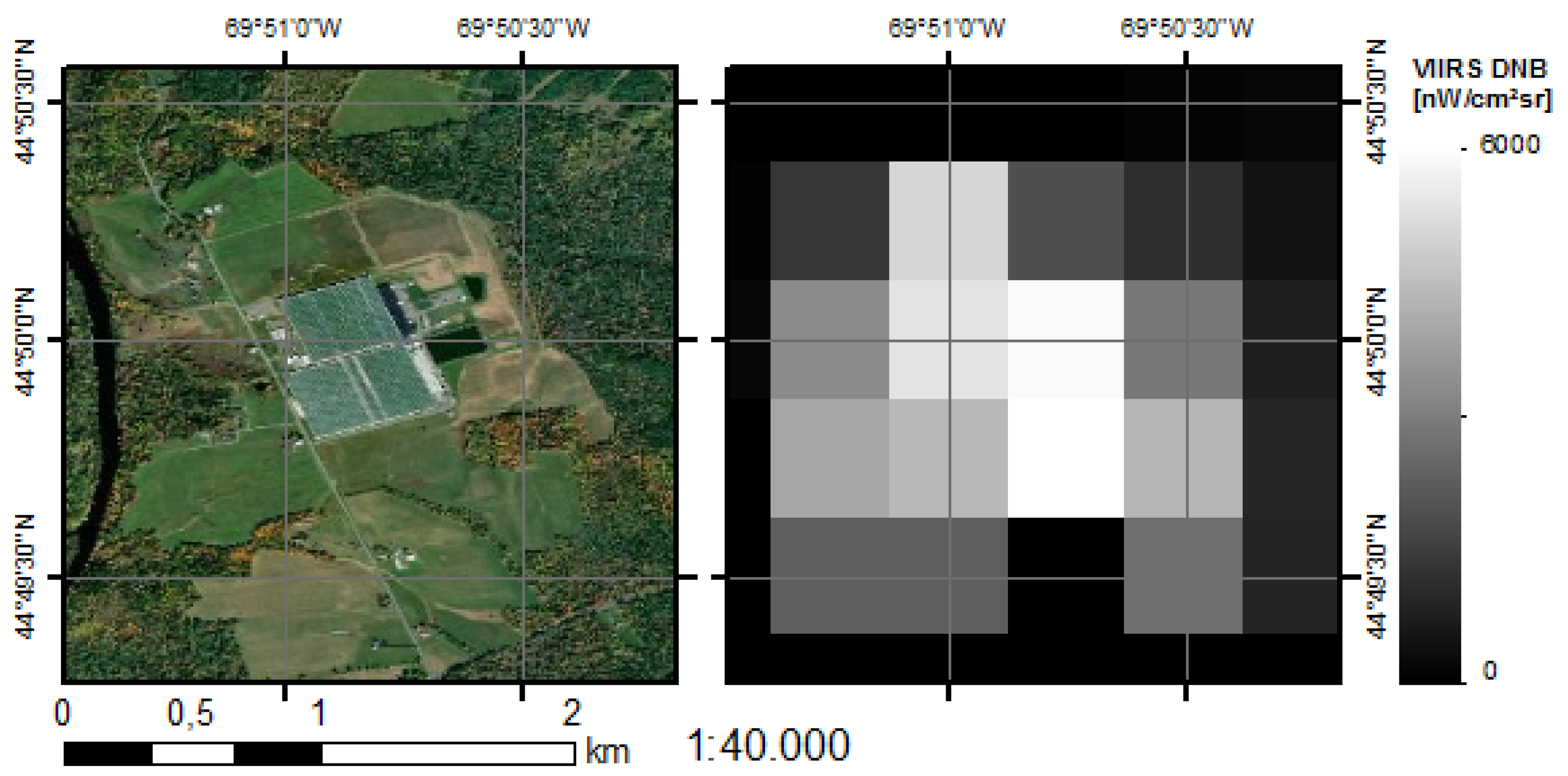
• Greenhouses Greenhouses were identified by searching for extraordinarily bright areas well separated from urban areas in the DNB data and by examining what buildings were present in Google Maps imagery. Large greenhouses typically appear as rectangular buildings or groups of buildings with transparent roofs. Greenhouses are among the brightest of all objects visible in the DNB data, with observed radiances often in the thousands of nW/cm${}^2$sr (Figure 2).

The sites are defined by their latitude and longitude. The complete list of sites (with the exception of flares) is available in the data and code supplement [48]. The sites were chosen without information regarding lighting types at the sites or whether they had experienced lighting changes. In fact, given the large number of sites, it must be expected that nearly all sites experienced changes in their installed lighting during the observation period. Even if new lighting systems are not installed, individual lamps typically decrease their light output over time, and in most cases failing lamps are exchanged for new (often slightly brighter) replacements. Since the aim of the study is to examine the stability of night light emissions, we do not impose any stability criterion on the data from the sites.

2.2. Night Light Data

Monthly composites of DNB data from April 2012 to September 2017 were downloaded from the National Oceanic and Atmospheric Administration (NOAA) [49]. The DNB has an intrinsic spatial resolution of ∼750 m (pixel area of ∼0.56 km${}^2$) [50], but the monthly composite data are reprojected by NOAA onto a 15 arc-second grid. These composites are based on multiple observations taken on clear nights throughout the month. NOAA identifies cloud cover via infrared observations on the same satellite, and nights with significant moonlight are not included in the composites [20]. Two sets of files are available from NOAA, which differ based on how stray light shining on the satellite sensor is handled. We selected the datasets in which observations where satellite sensor was exposed to stray light are rejected. For this reason, and due to the eventual presence of twilight at the overpass time of ∼01:30, many of the sites at northern latitudes do not have reported data during summer months (April–September).

2.3. Analysis

The analysis was performed using custom Python code [48]. For each monthly composite n, the DNB radiance $L_{s,n}$ (in nW/cm${}^2$sr) for each site s was written to an ASCII data file, as was the average radiance for the selected pixel and its four adjacent pixels. A separate Python routine then analyzed the data.

For each site, months containing no data (due to stray light on the satellite sensor) were rejected, and the median ${\tilde{m}}_s$ of the remaining data was identified. The monthly radiance data for each site were scaled relative to this median, to provide a relative monthly radiance for each site $R_{s,n}=L_{s,n}/{\tilde{m}}_s$, so the median value of $R_{s,n}\equiv 1$ by construction. This is done to make it possible to directly compare sites with different average radiances: a site with a median radiance of ${\tilde{m}}_s=50$ nW/cm${}^2$sr that fluctuates to 55 in month n and a site with a median radiance of 100 nW/cm${}^2$sr that fluctuates to 110 in month n would both have $R_{s,n}=1.1$.

We then examined the distribution of $R_{s,n}$ for each of the classes. After sorting all of the $R_{s,n}$ for a given class c numerically, we measured the width $W_c$ between the observations that would correspond to $\pm 1\sigma$ if the data were normally distributed (i.e., the 15.9th and 84.1th percentile, covering two standard deviations $\sigma$). This method is more robust than directly measuring the standard deviation, as a small number of outlier months (e.g., due to power disruption after a storm) will not affect the width of the distribution.

For comparison, the standard deviations of all $R_{s,n}$ for each class were also calculated. As an additional check, this method was then repeated for two alternate datasets. The first used the mean value of the central pixel plus its four direct neighbors, instead of the single pixel corresponding to the site location. The second analyzed only data from the months of September, October, and November, which are generally the most stable times of year in the North American DNB datasets, with October and September being the most stable [51].

Some factors that produce changes in the radiance of pixels in the DNB composites affect neighboring pixels equally, while others are specific to the individual pixel. For example, cloud cover, atmospheric transparency, time of night, soil moisture, phenological status of plants, and calibration factors for the DNB are surely strongly correlated between nearby pixels. In contrast, the light emission patterns (i.e., local geometry), the DNB individual channel noise, and the actual changes in installed lighting should be less well correlated (at least at distances beyond about 1 km). We therefore examined the Pearson correlation coefficient in the temporal variation of the monthly DNB radiance at closely and widely separated sites, for the locations in

Table 2. Locations used to examine correlation.

Location 1	Location 2	Approximate Distance
Atlanta, GA Suburb	Atlanta, GA Downtown	5 km
Atlanta, GA Suburb	Birmingham, AL Suburb	230 km
Atlanta, GA Suburb	Jackson, MS suburb	560 km
Atlanta, GA Suburb	Houston, TX suburb	1100 km
Atlanta, GA Suburb	Alburquerque, NM Suburb	2000 km
Alburquerque, NM Suburb	Alburquerque, NM Downtown	5 km

. Note that, although multiple locations are being compared, we are in fact examining a temporal, not a geospatial, correlation. This is the reason Pearson’s correlation coefficient is used rather than, e.g., Moran’s I. Lower latitude locations were chosen to maximize available data and minimize potential snow cover effects.

3. Results and Discussion

3.1. Stability of Lighting Classes

For each class, we compare a normal distribution with mean 1.0 and standard deviation of $W_c/2$ to a histogram of the median-corrected monthly observations $R_{s,n}$ for all months (n) and sites (s) in the class (Figure 3). The distributions are not normal, particularly in the high side tail (likely due to the increased surface albedo with snow). Nevertheless, for most classes and in most months, the data are reasonably well approximated by a Gaussian distribution. The exceptions to this are flares and greenhouses, which are not at all normally distributed.

The typical monthly variation in radiance, and the degree to which the distribution width $W_c$ matches 2$\sigma$, is shown in Figure 4. Urban and suburban areas, airports, and prisons had the narrowest distributions, at $W_c/2\approx$ 20%. The variations were larger for ship ports, stadiums, power plants, and bridges, which had $W_c/2\approx$ 30%. The radiance reported for natural areas in the DNB monthly composites is presumably due to a combination of sensor noise and natural light including dim moonlight, airglow [52,53], and, at high latitudes, aurora. The remote regions in Alaska were thus imaged through a brighter atmosphere (Figure 5) and perhaps as a result were relatively less affected by sensor noise. Finally, flares and greenhouses are simply not stable sources. The spike at zero in the distribution for greenhouses (Figure 3) suggests that in many cases they may have been constructed or first lit during the course of the study or were not lit during some months. Flares were observed to be highly variable and are discussed further later in the text. When only the more stable autumn months were considered, the distribution width $W_c$ decreased slightly in nearly all cases, but the overall conclusions were similar (Figure 4).

The analysis described above contains a thus far unstated assumption that the month-to-month variation in the observed radiance of a source is independent of the average radiance of the source. In order to test this, we calculated the width $W_{c,r}$ of the observed radiance distribution (in nW/cm${}^2$sr) as the difference between the 15.9th and 84.1th percentile observation for each individual site. If the data were normally distributed, this would be twice the standard deviation of the data.

The observations of $W_{c,r}/2\approx \sigma$ are plotted against the median radiance for each individual site (excluding flares), on a log–log plot (Figure 6). It is immediately apparent that, in many cases, typical monthly variation is roughly proportional to total radiance. On the other hand, (presumably unlit) wilderness areas appear to have larger variation, as do greenhouses. In the case of unlit or dimly lit areas, this likely indicates that sensor noise (e.g., digitization noise) or variation in natural light (e.g., airglow) dominates over effects related to the emitted artificial light (e.g., the overpass time, the atmospheric condition, and the imaging angle). For the greenhouses, the large variation is due to the greenhouses being unlit during some of the study period. In some cases, this may be because the greenhouse was only built partway through the study period, but we have also noted that some greenhouses were unlit during the summer months.

We performed two linear regression fits on the logarithm of the radiance data: one using data for all sites with the exception of flares, wilderness areas, and greenhouses, and one fit only to the urban sites. This fit can be transformed to provide an estimate of the typical variation in the monthly data $W_{c,r}/2$ as a function of median observed radiance at the site ${\tilde{m}}_s$. The (solid blue) fit to the larger set of sites returned $W_{c,r}/2=0.34{\tilde{m}}_s^{0.92}$. The (dashed purple) fit to urban locations returned $W_{c,r}/2=0.18{\tilde{m}}_s^{1.02}$. The fit to urban locations is consistent with the variation of month-to-month radiance being independent of site radiance. This fit sets an approximate lower limit on the monthly variation that can be expected from any given site.

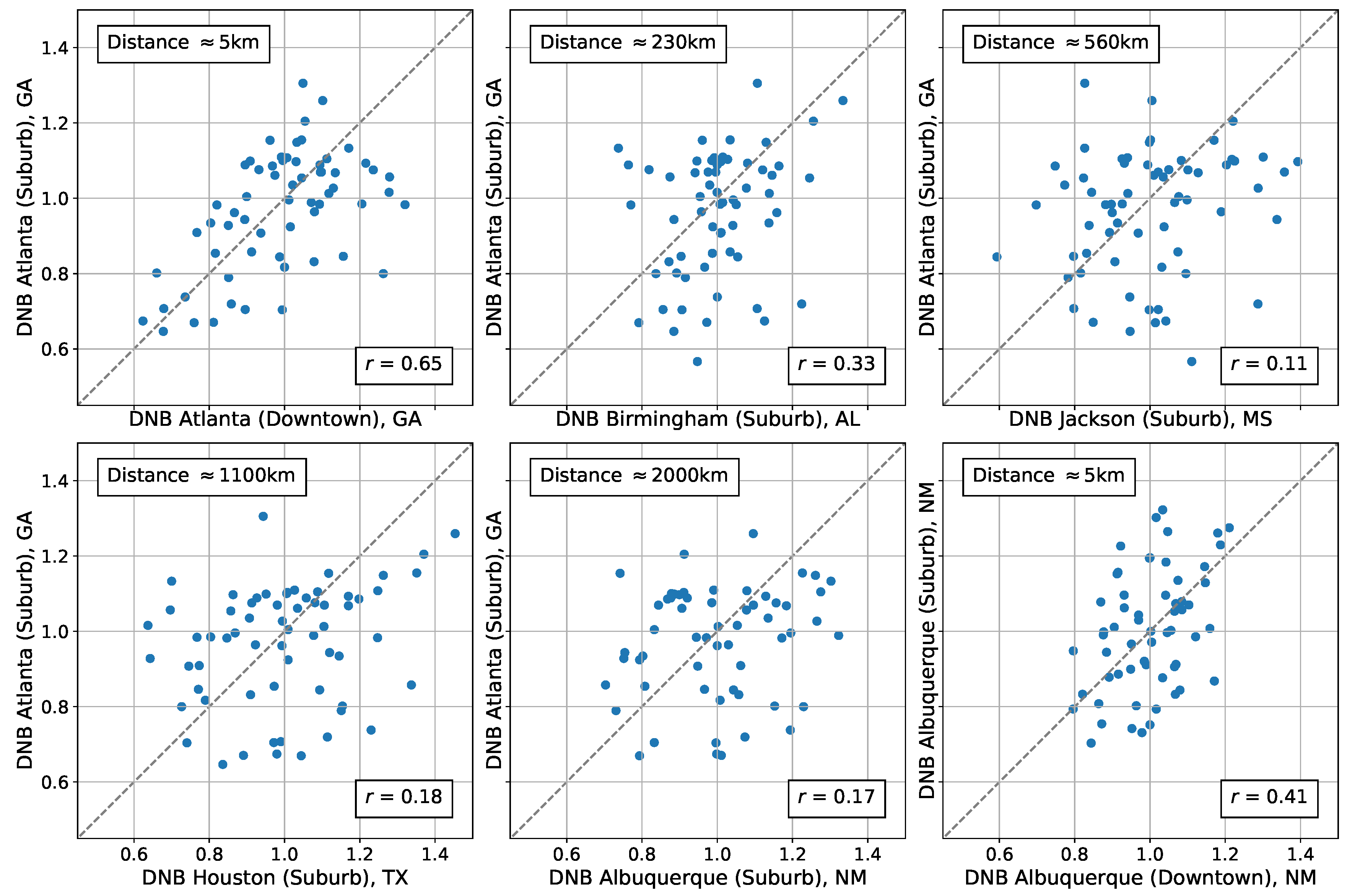
3.2. Temporal Correlations at Geographically Separated Sites

Some of the sources of month-to-month variation in observed radiance affect large areas of the globe similarly (e.g., the calibration and sensitivity of the DNB sensor and the seasonal variations), while others will be regional (weather), and some more local (e.g., imaging angle). If the main source of variation in DNB data was due to an instrumental effect (e.g., gain or calibration parameters), distant sites would experience strongly correlated variations. If, on the other hand, the main source of variation was due to local or regional effects, the correlations should decrease with distance.

The temporal correlation between radiance changes (relative to mean radiance) for a selection of suburban and urban sites is shown in Figure 7. At a distance of approximately 5 km, the month-to-month changes in radiance are quite obviously correlated (Pearson’s r of 0.41 and 0.65), demonstrating the presence of spatial autocorrelation in the temporal variation. At a distance of a few hundred km, the data were still somewhat correlated (r = 0.33), while at large distances they were only weakly correlated (r = 0.11, 0.17, and 0.18). The main source of variation in the DNB monthly composites therefore does not appear to be due to sensor calibration or gain.

During review, one of the reviewers pointed out that Figure 7 is reminiscent of Tobler’s “First Law of Geography,” which states that “everything is related to everything else, but near things are more related than distant things” [54]. Analyzing the root causes of the variation is beyond the scope of this paper, but it is worth considering for a moment how geographical closeness can affect these variations. While some atmospheric effects affect large scales (e.g., Sahara dust, and smoke), other effects can be highly local, either due to local emissions or micro climates. Similarly, the temporal changes in plant phenology and soil moisture that affect light emissions are correlated at large distances (i.e., seasons) but are much more strongly correlated at local scales. At short distances, the structures of buildings and streets are also more strongly correlated, and local topography can lead to strongly spatially correlated differences in radiance in DNB images (e.g., Kai Pong Tong has demonstrated very strong examples of this effect along coastlines, but this work has not yet been published).

The data presented in Figure 7 suggest that, when summing the light from a large area, such as a large country or a continent, variations from one region to another will tend to cancel each other out, leading to more stable sums. On the other hand, when summing the light from smaller regions, such as an individual city, one must expect spatially correlated fluctuations and therefore larger uncertainty on the observed radiance. An example of an extreme variation in a small area in a single monthly composite was recently reported for the city-state of Bremen in Germany [55]. These outliers would be of concern for studies that depend on time series in small areas, such as evaluating economic changes in individual cities (e.g., [56]), or epidemiological studies using satellite observed radiance as an exposure proxy for human exposure to artificial light (e.g., [57]).

To test the impact of considering multiple rather than single pixels in the DNB monthly composites, we repeated the analyses including the adjacent four pixels. The mean of five pixels was used as $L_{s,n}$ in place of the observation for a single pixel. The month-to-month variation was slightly reduced for all site types with the exception of wilderness areas. However, the reduction in variation was in most cases not as large as the reduction obtained by limiting the analysis to autumn months. These data are presented in Figure S1.

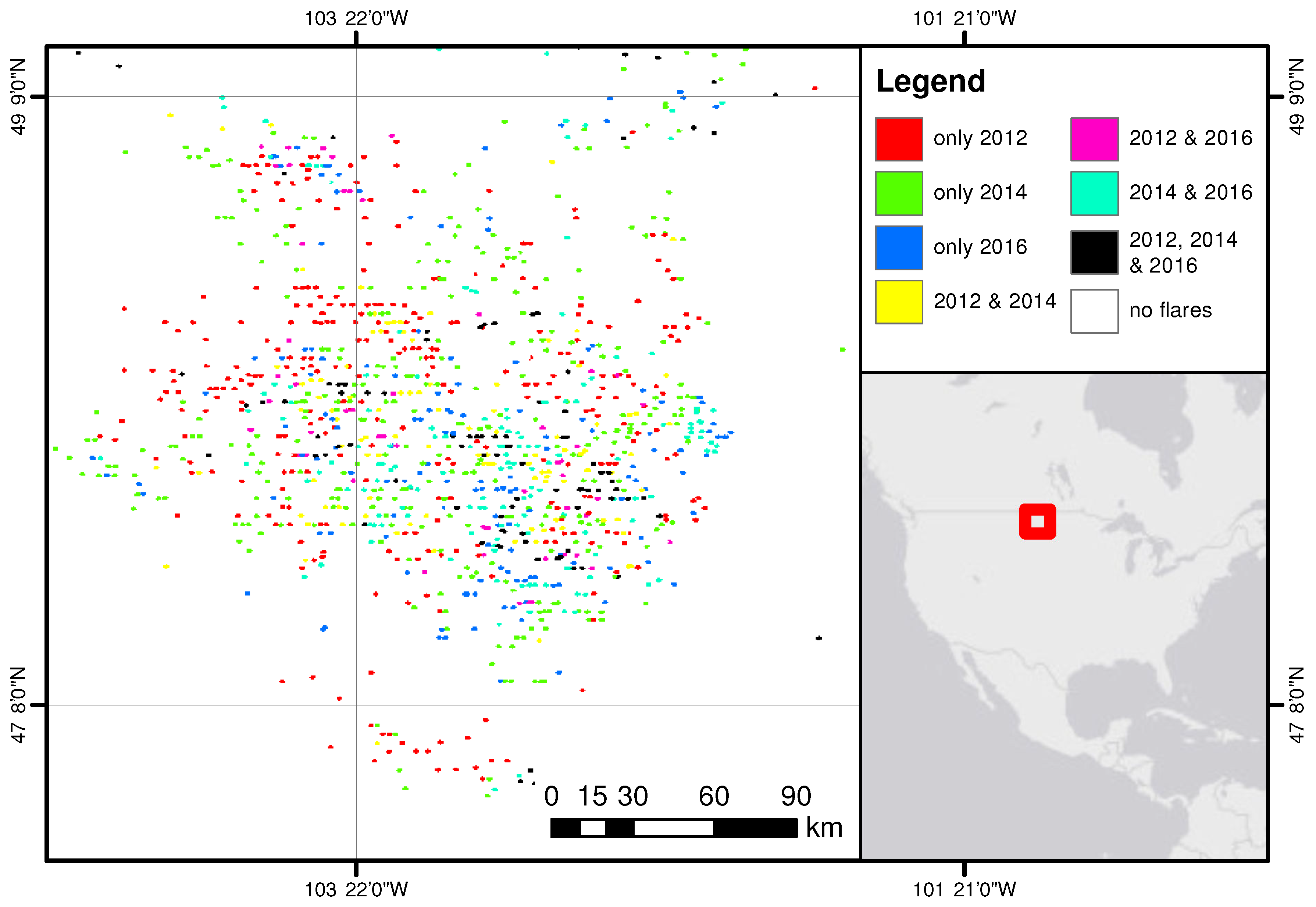
3.3. Stability of Gas Flaring

Light emitted from gas flares was the least stable out of all the classes examined. To a large extent, this was due to flares being present in only a portion of the dataset. This can be seen, for example, in the years in which individual flares produced light. We examined the mean radiance for pixels within 750 m of identified flaring sites. In Figure 8, flares that were lit above 10 nW/cm${}^2$sr in October 2012, 2014, and 2016 are shown in black, while flares lit in only one or two of those years are shown in color. While the entire Bakken region has appeared to be rather continuously lit throughout the DNB time series, the locations of the light sources are in fact changing from year to year.

3.4. Seasonal Changes

Seasonal effects in night light data are well known (e.g., [18,58]). The most important seasonal effect is due to snow cover raising the reflectivity of the ground surface, and an increase in winter months is visible for all of the brightly lit classes examined here (Figures S2–S4). The impact of leaf cover is not as well understood. We note that, for downtown and suburb locations, November is brighter than October (Figure S3), but detailed analysis is beyond the scope of this study. The brightening effects of snow are extremely strong, so it is advisable for analyses of areas at northern latitudes to restrict their time frame to autumn months.

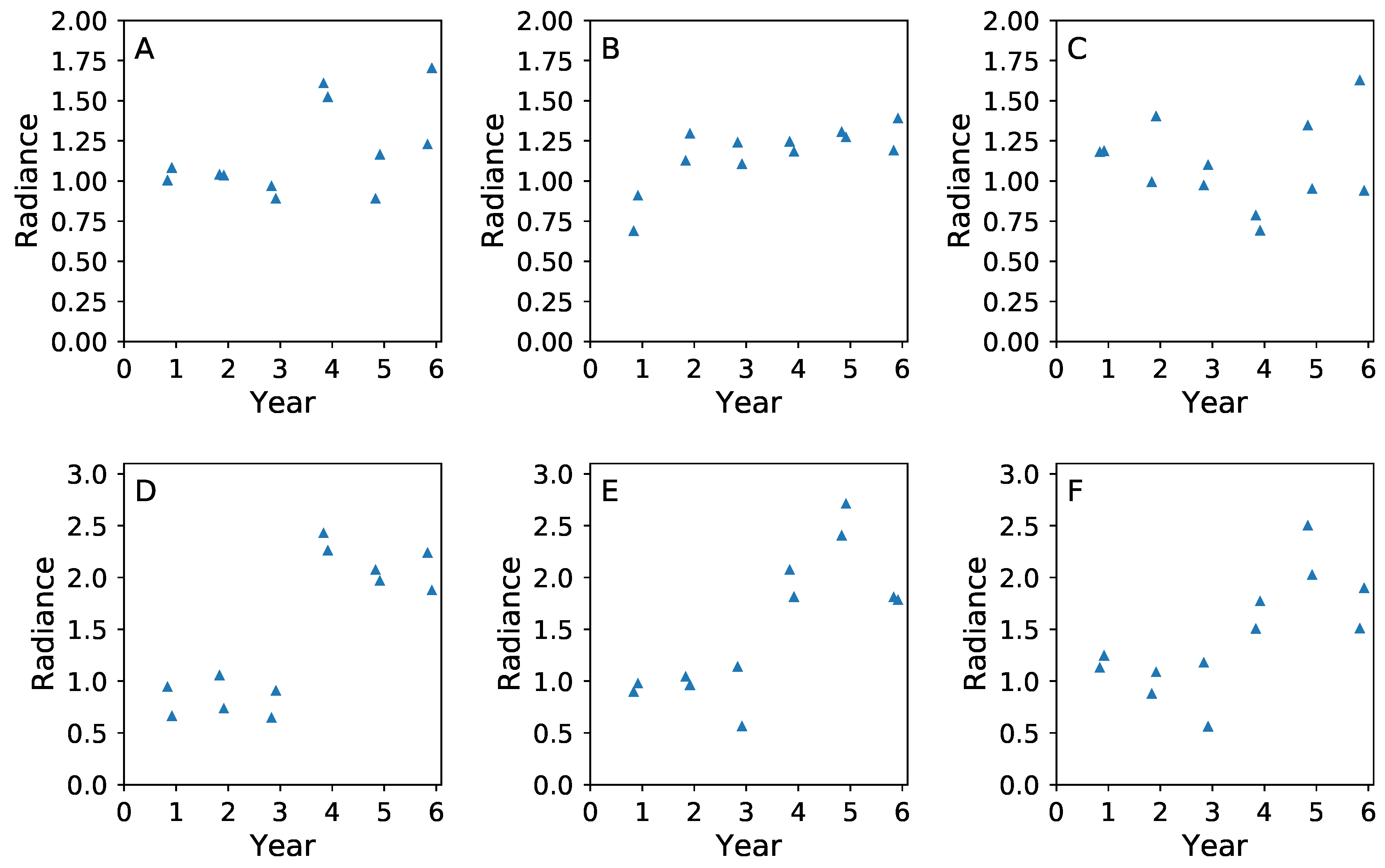
3.5. Understanding DNB Time Series

The approximately 15–20% variation in observed DNB radiance from month to month places a limit on the level of change in light emission that can be positively detected by the DNB. Dramatic changes, such as the appearance or disappearance of a lamp, are readily seen, as in the example of the Bakken flares above, through an intervention to intentionally eliminate upward light emissions [9] or through long-term power outages. However, more moderate changes, such as may be expected from a conversion to LED lamps or the addition of new advertising or facade lighting in an already bright urban center, may be less obvious.

We produced simulated datasets of step function changes in light emission to highlight how the variation affects the trajectory of time series (Figure 9). During the first three years, the data are normally distributed around a value of 1, while during the final three years, the data are normally distributed around either 1.3 (Figure 9A–C) or 2 (Figure 9D–F). In all cases, the standard deviation was set to 20%. If emissions change suddenly by a factor of two or more, this can be clearly observed as a step function in the time series (Figure 9D–F). When the change is smaller, however, the interpretation is much less clear. For example, in Figure 9B,C, it would be unclear whether the data ought to be fit with a step function or a linear increase.

At the scale of a few meters, installed lighting can change both in a stepwise manner (e.g., with the introduction of new light sources at a newly opened business) and in a more gradual manner (e.g., with the aging of light sources). At the 0.5 km${}^2$ scale of DNB, both processes may be occurring simultaneously, especially for pixels that cover areas where multiple actors are responsible for individual lighting decisions. The question of how to fit the time series and how to describe the results of such fits is therefore difficult, particularly in the case when there is a sudden jump near the start or end of the time series. A linear or exponential fit may not be a good representation of the underlying “true” light emissions, but a ratio of end to start radiance is problematic because it is subject to the largest possible month-to-month variation.

The situation is even more problematic in high latitude regions, for which analyses must usually be restricted to data taken in October and November (to ensure no stray light on the sensor and no snow on the ground). While changes in the radiance of a factor 2 or more are still clear (Figure 10D–F), smaller changes become even more ambiguous and liable to misinterpretation. For example, Figure 10B incorrectly appears to show a clear step function taking place during Year 1, while no trend at all is apparent in Figure 10C.

When light emissions from large areas are summed (for example, to examine trends in cities, states, or countries), the sum may reasonably be expected to be more stable than what we observe for individual pixels. For example, we observed that the variation in the sum of five pixels is more stable than for the individual central pixel (Figure S1) and that the variations observed for distantly separated points are only partially correlated (Figure 7). On the other hand, this study considered only large-scale sources. It is possible that smaller spatial scale light sources may have a larger variation, and, in addition, the greater the area studied, the greater the likelihood that the area will include a high variability source, such as a greenhouse or flare.

One may therefore question whether previous studies of national and state level trends using DNB light emissions have drawn correct conclusions. For example, Kyba et al. [55] examined five-year time series of German federal states and claimed to observe changes on the level of –7% to +40%. Are such reports correct? The early indications are that, for a sufficiently large study areas, it appears possible to observe statistically significant differences in trends between different regions, provided that the differences are at least several percent (≥4%) per year [55]. As the length of the DNB time series grows, confidence in the validity of observed trends will be easier to establish (assuming the underlying trends in light emission continue). We intend to examine trends and variability at larger spatial scales and on daily rather than monthly timescales, continuing this discussion in future publications.

4. Conclusions

Variations in the month-to-month radiance observed by the DNB for several types of large light emitters in the USA and Canada are relatively well approximated by a normal distribution, with outliers on the high side due to snow cover. The standard deviation for the individual pixels of urban, suburban, airport, and prison sites examined is about 20% relative to the median. This is reduced to about 15% if only autumn months are considered. Other sources of light (e.g., ports, stadiums, and power plants) are slightly more variable, while greenhouses and flares are not at all stable. When multiple pixels around a site are averaged together, the month-to-month radiance is slightly reduced. However, in some cases this will make the study area larger than the site itself, and the reduction in variation by expanding the area is smaller than was achieved by restricting the data to autumn months.

At short distances (∼5 km), month-to-month radiance changes in pairs of sites are fairly strongly correlated (Pearson’s r up to 0.65). Month-to-month changes in radiance of sites at distances of several hundred kilometers are either weakly or not correlated. These results suggest that the DNB sensor and calibration factors are not the source of the variation. Instead, local factors such as the imaging angle, the time of night, or atmospheric parameters on the days when the data were acquired are presumably the main source of variation observed in DNB monthly composites. At the spatial scale of a single pixel, changes must be large (near factor 2) in order to be confidently observed. At larger spatial scales, it is likely that smaller changes in installed lighting can be observed, due to an averaging of variation over multiple pixels.

As the spatial resolution of a night light sensor increases, so does the contrast of the scene (e.g., [32,59]). At high resolution, small differences in imaging direction can have a dramatic influence on the observed radiance (Figure 1), and the impact of scattering by aerosols will have a much stronger effect. These effects already limit the ability of the DNB to sense changes in installed lighting, and they will only become worse with new, higher-resolution instruments. It is therefore important to understand the causes of the variation in night light data in order to maximize the usefulness of existing and future night light sensors.

References

1. Elvidge, C.D.; Baugh, K.E.; Kihn, E.A.; Kroehl, H.W.; Davis, E.R. Mapping city lights with nighttime data from the DMSP Operational Linescan System. Photogramm. Eng. Remote Sens. 1997, 63, 727–734. [Google Scholar]
2. Lu, H.; Zhang, M.; Sun, W.; Li, W. Expansion Analysis of Yangtze River Delta Urban Agglomeration Using DMSP/OLS Nighttime Light Imagery for 1993 to 2012. ISPRS Int. J. Geo-Inf. 2018, 7, 52. [Google Scholar] [CrossRef]
3. Zhu, X.; Ma, M.; Yang, H.; Ge, W. Modeling the spatiotemporal dynamics of gross domestic product in China using extended temporal coverage nighttime light data. Remote Sens. 2017, 9, 626. [Google Scholar] [CrossRef]
4. Jiang, W.; He, G.; Long, T.; Liu, H. Ongoing Conflict Makes Yemen Dark: From the Perspective of Nighttime Light. Remote Sens. 2017, 9, 798. [Google Scholar] [CrossRef]
5. Levin, N.; Ali, S.; Crandall, D. Utilizing remote sensing and big data to quantify conflict intensity: The Arab Spring as a case study. Appl. Geogr. 2018, 94, 1–17. [Google Scholar] [CrossRef]
6. Li, X.; Li, D.; Xu, H.; Wu, C. Intercalibration between DMSP/OLS and VIIRS night-time light images to evaluate city light dynamics of Syria’s major human settlement during Syrian Civil War. Int. J. Remote Sens. 2017, 38, 5934–5951. [Google Scholar] [CrossRef]
7. Gaston, K.J.; Duffy, J.P.; Bennie, J. Quantifying the erosion of natural darkness in the global protected area system. Conserv. Biol. 2015, 29, 1132–1141. [Google Scholar] [CrossRef] [PubMed]
8. Guetté, A.; Godet, L.; Juigner, M.; Robin, M. Worldwide increase in Artificial Light At Night around protected areas and within biodiversity hotspots. Biol. Conserv. 2018, 223, 97–103. [Google Scholar] [CrossRef]
9. Kyba, C.C.; Mohar, A.; Pintar, G.; Stare, J. Reducing the environmental footprint of church lighting: Matching facade shape and lowering luminance with the EcoSky LED. Int. J. Sustain. Light. 2017, 19, 132. [Google Scholar] [CrossRef]
10. Kyba, C.C.; Kuester, T.; de Miguel, A.S.; Baugh, K.; Jechow, A.; Hölker, F.; Bennie, J.; Elvidge, C.D.; Gaston, K.J.; Guanter, L. Artificially lit surface of Earth at night increasing in radiance and extent. Sci. Adv. 2017, 3, e1701528. [Google Scholar] [CrossRef] [Green Version]
11. Ghosh, T.; Powell, R.L.; Elvidge, C.D.; Baugh, K.E.; Sutton, P.C.; Anderson, S. Shedding light on the global distribution of economic activity. Open Geogr. J. 2010, 3, 147–160. [Google Scholar]
12. Ghosh, T.; Elvidge, C.D.; Sutton, P.C.; Baugh, K.E.; Ziskin, D.; Tuttle, B.T. Creating a global grid of distributed fossil fuel CO2 emissions from nighttime satellite imagery. Energies 2010, 3, 1895–1913. [Google Scholar] [CrossRef]
13. Jean, N.; Burke, M.; Xie, M.; Davis, W.M.; Lobell, D.B.; Ermon, S. Combining satellite imagery and machine learning to predict poverty. Science 2016, 353, 790–794. [Google Scholar] [CrossRef] [PubMed]
14. Kyba, C.; Ruhtz, T.; Lindemann, C.; Fischer, J.; Hölker, F. Two camera system for measurement of urban uplight angular distribution. In Proceedings of the International Radiation Symposium (IRC/IAMAS) Radiation Processes in the Atmosphere and Ocean (IRS2012), Berlin, Germany, 6–10 August 2012; AIP Publishing: Melville, NY, USA, 2013; Volume 1531, pp. 568–571. [Google Scholar]
15. Tong, K.P. On Observations of Artificial Light at Night from Ground and Space. Ph.D. Thesis, Universität Bremen, Bremen, Germany, 2017. [Google Scholar]
16. Kyba, C.C.M.; Ruhtz, T.; Fischer, J.; Hölker, F. Red is the New Black: How the Color of Urban Skyglow Varies with Cloud Cover. Mon. Not. R. Astron. Soc. 2012, 425, 701–708. [Google Scholar] [CrossRef]
17. Bará, S.; Rodríguez-Arós, Á.; Pérez, M.; Tosar, B.; Lima, R.C.; de Miguel, A.S.; Zamorano, J. Estimating the relative contribution of streetlights, vehicles and residential lighting to the urban night sky brightness. Light. Res. Technol. 2018. [Google Scholar] [CrossRef]
18. Levin, N. The impact of seasonal changes on observed nighttime brightness from 2014 to 2015 monthly VIIRS DNB composites. Remote Sens. Environ. 2017, 193, 150–164. [Google Scholar] [CrossRef]
19. Fu, D.; Xia, X.; Duan, M.; Zhang, X.; Li, X.; Wang, J.; Liu, J. Mapping nighttime PM2.5 from VIIRS DNB using a linear mixed-effect model. Atmos. Environ. 2018, 178, 214–222. [Google Scholar] [CrossRef]
20. Elvidge, C.D.; Baugh, K.; Zhizhin, M.; Hsu, F.C.; Ghosh, T. VIIRS night-time lights. Int. J. Remote Sens. 2017, 38, 5860–5879. [Google Scholar] [CrossRef] [Green Version]
21. Zeng, X.; Shao, X.; Qiu, S.; Ma, L.; Gao, C.; Li, C. Stability Monitoring of the VIIRS Day/Night Band over Dome C with a Lunar Irradiance Model and BRDF Correction. Remote Sens. 2018, 10, 189. [Google Scholar] [CrossRef]
22. Román, M.O.; Wang, Z.; Sun, Q.; Kalb, V.; Miller, S.D.; Molthan, A.; Schultz, L.; Bell, J.; Stokes, E.C.; Pandey, B.; et al. NASA’s Black Marble nighttime lights product suite. Remote Sens. Environ. 2018, 210, 113–143. [Google Scholar] [CrossRef]
23. Román, M.O.; Stokes, E.C. Holidays in lights: Tracking cultural patterns in demand for energy services. Earths Future 2015, 3, 182–205. [Google Scholar] [CrossRef] [PubMed] [Green Version]
24. Kohiyama, M.; Hayashi, H.; Maki, N.; Higashida, M.; Kroehl, H.; Elvidge, C.; Hobson, V. Early damaged area estimation system using DMSP-OLS night-time imagery. Int. J. Remote Sens. 2004, 25, 2015–2036. [Google Scholar] [CrossRef]
25. Cao, C.; Shao, X.; Uprety, S. Detecting light outages after severe storms using the S-NPP/VIIRS day/night band radiances. IEEE Geosci. Remote Sens. 2013, 10, 1582–1586. [Google Scholar] [CrossRef]
26. Mann, M.L.; Melaas, E.K.; Malik, A. Using VIIRS day/night band to measure electricity supply reliability: Preliminary results from Maharashtra, India. Remote Sens. 2016, 8, 711. [Google Scholar] [CrossRef]
27. Sánchez de Miguel, A.; Zamorano, J.; Gómez Castaño, J.; Pascual, S. Evolution of the energy consumed by street lighting in Spain estimated with DMSP-OLS data. J. Quant. Spectrosc. Radiat. Transfer 2014, 139, 109–117. [Google Scholar] [CrossRef] [Green Version]
28. Estrada-García, R.; García-Gil, M.; Acosta, L.; Bará, S.; Sanchez-de Miguel, A.; Zamorano, J. Statistical modelling and satellite monitoring of upward light from public lighting. Light. Res. Technol. 2016, 48, 810–822. [Google Scholar] [CrossRef] [Green Version]
29. De Miguel, A.S. Variación Espacial, Temporal y Espectral de la Contaminación Lumınica y Sus Fuentes: Metodologıa y Resultados. Ph.D. Thesis, Universidad Complutense de Madrid, Madrid, Spain, July 2015. [Google Scholar]
30. Sánchez de Miguel, A.; Zamorano, J.; Pascual, S.; López Cayuela, M.; Ocaña, F.; Challupner, P.; Gómez Castaño, J.; Fernández-Renau, A.; Gómez, J.; de Miguel, E. ISS nocturnal images as a scientic tool against Light Pollution: Flux calibration and colors. In Highlights of Spanish Astrophysics VII, Proceedings of the X Scientific Meeting of the Spanish Astronomical Society (SEA), Valencia, Spain, 9–13 July 2012; Sociedad Española de Astronomía: Costa del Sol, Spain; Volume 1, pp. 916–919.
31. Kyba, C.; Garz, S.; Kuechly, H.; de Miguel, A.S.; Zamorano, J.; Fischer, J.; Hölker, F. High-Resolution Imagery of Earth at Night: New Sources, Opportunities and Challenges. Remote Sens. 2015, 7, 1–23. [Google Scholar] [CrossRef] [Green Version]
32. Kuechly, H.U.; Kyba, C.C.M.; Ruhtz, T.; Lindemann, C.; Wolter, C.; Fischer, J.; Hölker, F. Aerial survey of light pollution in Berlin, Germany, and spatial analysis of sources. Remote Sens. Environ. 2012, 126, 39–50. [Google Scholar] [CrossRef]
33. Hale, J.D.; Davies, G.; Fairbrass, A.J.; Matthews, T.J.; Rogers, C.D.; Sadler, J.P. Mapping lightscapes: Spatial patterning of artificial lighting in an urban landscape. PLoS ONE 2013, 8, e61460. [Google Scholar] [CrossRef] [Green Version]
34. Fotios, S.; Gibbons, R. Road lighting research for drivers and pedestrians: The basis of luminance and illuminance recommendations. Light. Res. Technol. 2018, 50, 154–186. [Google Scholar] [CrossRef] [Green Version]
35. Kocifaj, M. Towards a comprehensive city emission function (CCEF). J. Quant. Spectrosc. Radiat. 2018, 205, 253–266. [Google Scholar] [CrossRef]
36. National Oceanic and Atmospheric Administration. Global Gas Flaring Observed from Space. 2012–2017. Available online: https://ngdc.noaa.gov/eog/viirs/download_global_flare.html (accessed on 11 November 2017).
37. Bureau, U.S.C. Guide to State and Local Census Geography. 2010. Available online: https://www2.census.gov/geo/pdfs/reference/guidestloc/All_GSLCG.pdf (accessed on 28 February 2018).
38. Federal Aviation Administration. Enplanements at All Commercial Service Airports (by Rank). 2017. Available online: https://www.faa.gov/airports/planning_capacity/passenger_allcargo_stats/passenger/media/cy16-commercial-service-enplanements.pdf (accessed on 28 February 2018).
39. Statistics Canada. Passengers eNplaned and Deplaned on Selected Services—Top 50 Airports. 2016. Available online: http://www.statcan.gc.ca/pub/51-203-x/2015000/t002-eng.htm (accessed on 28 February 2018).
40. American Association of Port Authorities. Port Industry Statistics—U.S. Port Ranking by Cargo Tonnage 2013. 2014. Available online: http://www.aapa-ports.org/unifying/content.aspx?ItemNum-ber=21048 (accessed on 1 March 2018).
41. Transport Canada. 2018. Available online: http://www.tc.gc.ca/en/services/marine/ports-harbours/list-canada-port-authorities.html (accessed on 2 March 2018).
42. Misachi, J. The Largest Sports Stadiums in Canada. 2017. Available online: https://www.worldatlas.com/articles/which-are-the-largest-sports-stadiums-in-canada.html (accessed on 1 March 2018).
43. US Energy Information Administration. Form EIA-860 Detailed Data—EIA-923 Monthly Generation and Fuel Consumption Time Series File, 2016 Final Revision. 2017. Available online: https://www.eia.gov/electricity/data/eia860/index.html (accessed on 3 March 2018).
44. US Energy Information Administration. State Nuclear Profiles. 2012. Available online: https://www.eia.gov/electricity/data/eia860/index.html (accessed on 3 March 2018).
45. US Department of Homeland Security. Prison Boundaries. 2017. Available online: https://hifld-geoplatform.opendata.arcgis.com/datasets/prison-boundaries/data (accessed on 31 October 2017).
46. Elvidge, C.D.; Zhizhin, M.; Baugh, K.; Hsu, F.C.; Ghosh, T. Methods for global survey of natural gas flaring from visible infrared imaging radiometer suite data. Energies 2016, 9, 14. [Google Scholar] [CrossRef]
47. United States Department of Agriculture Forest Service. Wilderness Areas: Legal Status. 2017. Available online: https://data.fs.usda.gov/geodata/edw/datasets.php?dsetCategory=boundaries (accessed on 2 November 2017).
48. Coesfeld, J.; Kyba, C. Software Supplement to: “Variation of Individual Location Radiance in VIIRS DNB Monthly Composite Images”. V. 1.0. GFZ Data Services. 2018. [Google Scholar] [CrossRef]
49. National Centers for Environmental Information, National Oceanic and Atmospheric Administration. VIIRS DNB Nighttime Lights Composites. 2012–2017. Available online: https://www.ngdc.noaa.gov/eog/viirs/download_dnb_composites.html (accessed on several dates between 10 February 2015 and 10 October 2017).
50. Miller, S.D.; Straka, W.; Mills, S.P.; Elvidge, C.D.; Lee, T.F.; Solbrig, J.; Walther, A.; Heidinger, A.K.; Weiss, S.C. Illuminating the Capabilities of the Suomi National Polar-Orbiting Partnership (NPP) Visible Infrared Imaging Radiometer Suite (VIIRS) Day/Night Band. Remote Sens. 2013, 5, 6717–6766. [Google Scholar] [CrossRef] [Green Version]
51. Kleinsteuber, F.A. Testing Stability of VIIRS DNB Night Lights Data in the United States of America. Master’s Thesis, Universität Trier, Trier, Germany, February 2017. [Google Scholar]
52. Miller, S.; Mills, S.; Elvidge, C.; Lindsey, D.; Lee, T.; Hawkins, J. Suomi satellite brings to light a unique frontier of nighttime environmental sensing capabilities. Proc. Natl. Acad. Sci. USA 2012, 109, 15706–15711. [Google Scholar] [CrossRef] [PubMed] [Green Version]
53. Noll, S.; Kausch, W.; Barden, M.; Jones, A.; Szyszka, C.; Kimeswenger, S.; Vinther, J. An atmospheric radiation model for Cerro Paranal-I. The optical spectral range. Astron. Astrophys. 2012, 543, A92. [Google Scholar] [CrossRef]
54. Tobler, W.R. A computer movie simulating urban growth in the Detroit region. Econ. Geogr. 1970, 46, 234–240. [Google Scholar] [CrossRef]
55. Kyba, C.C.; Kuester, T.; Kuechly, H.U. Changes in outdoor lighting in Germany from 2012–2016. Int. J. Sustain. Light. 2017, 19, 112–123. [Google Scholar] [CrossRef]
56. Lu, Y.; Coops, N.C. Bright lights, big city: Causal effects of population and GDP on urban brightness. PLoS ONE 2018, 13, e0199545. [Google Scholar] [CrossRef]
57. James, P.; Bertrand, K.A.; Hart, J.E.; Schernhammer, E.S.; Tamimi, R.M.; Laden, F. Outdoor light at night and breast cancer incidence in the Nurses’ Health Study II. Environ. Health Perspect. 2017, 125, 087010. [Google Scholar] [CrossRef]
58. Falchi, F. Campaign of sky brightness and extinction measurements using a portable CCD camera. Mon. Not. R. Astron. Soc. 2011, 412, 33–48. [Google Scholar] [CrossRef]
59. Jiang, W.; He, G.; Long, T.; Guo, H.; Yin, R.; Leng, W.; Liu, H.; Wang, G. Potentiality of Using Luojia 1-01 Nighttime Light Imagery to Investigate Artificial Light Pollution. Sensors 2018, 18, 2900. [Google Scholar] [CrossRef] [PubMed]
60. Coesfeld, J. Nachtaufnahmen in der Fernerkundung: Überprüfung der Variabilität des VIIRS Day/Night Bands Anhand Einzelner Standorte. Bachelor’s Thesis, Universität Potsdam, Potsdam, Germany, July 2018. [Google Scholar]
Figure 1. Visibility of facades depends on perspective. The top image is a crop of an photograph taken from the North, so North facing facades such as that highlighted in the oval are visible. The bottom image was taken from the South, so the North facing sides of buildings therefore appear dark. Similar effects are visible on many other buildings. Photos taken by Alejandro Sánchez de Miguel and the Freie Universität Berlin during the EU COST Action ES1204 LoNNe.
Remotesensing 10 01964 g001
Figure 2. Greenhouse complex in the US state of Maine (44 49 57.7 N, 68 50 52.4 W). The image shows both the extreme brightness of the greenhouse and how the light is not restricted to within a single pixel in the monthly composite.
Remotesensing 10 01964 g002
Figure 3. Radiance relative to the site median ( R s , n ) for all sites and months within each given class. The curve shows a normal distribution based on the data, but is not a fit (see text). The dotted white lines show the location of the 15.9th and 84.1th percentile. The wilderness class was divided into wilderness areas in Alaska (Wild. N) versus in the contiguous US states (Wild. S). Note that the horizontal axis of the bottom four panels covers larger ranges than the top eight panels.
Remotesensing 10 01964 g003
Figure 4. Typical monthly variation in observed radiance for each of the classes. In each case, W c / 2 is shown in dark blue, and the sample standard deviation σ in light blue. The left plot includes data from all months, the right plot includes data only from the autumn months.
Remotesensing 10 01964 g004
Figure 5. Scatterplot of average radiance of pixels in wilderness areas against latitude. Both the mean and median are shown. The wilderness areas in Alaska are more brightly lit on average, presumably due to auroral emissions.
Remotesensing 10 01964 g005
Figure 6. Relationship between the typical month-to-month variation in radiance to the mean radiance for all sites with the exception of flares, plotted on a log–log scale. The lines show linear regressions on the logarithmic values.
Remotesensing 10 01964 g006
Figure 7. Monthly radiance relative to the median of all months is shown for pairs of sites at different distances. The first five plots compare sites to the suburban site in Atlanta, Georgia, the final plot is for two locations in Albuquerque. The first and final plots compare urban to suburban radiance in a single city, while the other plots compare pairs of suburban locations.
Remotesensing 10 01964 g007
Figure 8. Active gas flares in the Bakken oil region during 2012, 2014, and 2016. Sites with an average radiance above 10 nW/cm 2 sr were considered to be lit. Map data in the bottom right panel ©OpenStreetMap contributors
Remotesensing 10 01964 g008
Figure 9. Simulated six-year DNB time series. In the top plots, the average radiance changes from 1 to 1.3 at the start of Year 3. In the bottom plots, the average radiance changes from 1 to 2 at the start of Year 3. A running centered 13 month mean is overlaid.
Remotesensing 10 01964 g009
Figure 10. Simulated six-year DNB time series showing only data for October and November. The points shown are drawn directly from the simulated dataset shown in Figure 9.
Remotesensing 10 01964 g010