Yield Estimation of Paddy Rice Based on Satellite Imagery: Comparison of Global and Local Regression Models

Abstract

Precisely estimating the yield of paddy rice is crucial for national food security and development evaluation. Rice yield estimation based on satellite imagery is usually performed with global regression models; however, estimation errors may occur because the spatial variation is not considered. Therefore, this study proposed an approach estimating paddy rice yield based on global and local regression models. In our study area, the overall per-field data might not available because it took lots of time and manpower as well as resources. Therefore, we gathered and accumulated 26 to 63 ground survey sample fields, accounting for about 0.05% of the total cultivated areas, as the training samples for our regression models. To demonstrate whether the spatial autocorrelation or spatial heterogeneity exists and dominates the estimation, global models including the ordinary least squares (OLS), support vector regression (SVR), and the local model geographically weighted regression (GWR) were used to build the yield estimation models. We obtained the representative independent variables, including 4 original bands, 11 vegetation indices, and 32 texture indices, from SPOT-7 multispectral satellite imagery. To determine the optimal variable combination, feature selection based on the Pearson correlation was used for all of the regression models. The case study in Central Taiwan rendered that the error rate was between 0.06% and 13.22%. Through feature selection, the GWR model’s performance was more relatively stable than the OLS model and nonlinear SVR model for yield estimation. Where the GWR model considers the spatial autocorrelation and spatial heterogeneity of the relationships between the yield and the independent variables, the OLS and nonlinear SVR models lack this feature; this led to the rice yield estimation of GWR in this study be more stable than those of the other two models.

1. Introduction

With the improvement of agricultural science and technology, pests, bacteria, and environmental factors are having less of an effect on the growth of rice. On the authority of the FAOSTAT database from Food and Agriculture Organization of the United Naitons, the harvested area and yield of paddy rice reached a historic high of 145.4 million hectares and 672.5 million tons in Asia in 2013. Although the harvested area decreased by 2.9%, the yield only slightly decreased by 0.1% from 2013 to 2016 [1]. The aforementioned data infers the growth of the rice yield per unit area, and also reflects the development of the national economy. Therefore, precisely mapping the cultivation area and estimating the yield of paddy rice are both crucial for national food security and national development evaluation.

Concerning the paddy rice yield, ground-based field survey is still an essential process for regional and national level estimation, although this necessary survey is usually thought of as being time-consuming, subjective [2], and costly [3]. By utilizing data well, such as ground survey data, the rice yield can be estimated in multiple ways. Remote sensing is a common method of estimation. However, in many studies, satellite data selection, application, analysis, and verification methods differ from one another; therefore, effectively attenuating the limitations of previous studies is an essential aspect of estimation.

Numerous studies used and combined satellite imagery with regression models for the yield estimation of agricultural crops [4,5,6]. However, early rice yield estimation studies used nonderived elements for regression analysis; for instance, one study employed the reflection spectrum and the actual rice yield [7,8]. However, this method is only applicable to the spatial distribution of the relative yield of rice. Some studies have consequently used the normalized difference vegetation index (NDVI), ratio vegetation index (RVI), transformed vegetation index (TVI), or meteorological variables to build yield estimation models [4,5,6] towards establishing a regression model for rice yield estimation. The prerequisite of using most vegetation indices is radiometric calibration or surface reflectance retrieval of remote sensing images to decrease the influence of atmospheric effects. Being unable to achieve the prerequisite may limit the usage of vegetation indices for yield estimation.

With the improved use of a single element for regression analysis, to avoid the limitations of acquisition time and space effects on imagery, previous studies have combined aerial photographs equipped to establish regression models with visible, near-infrared, and vegetation indices [9,10]. Some research used ground-based remotely sensed high-resolution spectral reflectance, the leaf area index (LAI), and the actual rice yield to establish a regression model for predicting rice yield [9,11]. The data were divided and extracted in as many ways as possible, so as to improve the observation accuracy. Vegetation indices are the best data extraction representative with the widest coverage of land; thus, they constitute a crucial factor in many studies. Researchers have added multiple bands, vegetation indices, and rice yields in order to establish a multiple regression model for predicting rice yield [9,12,13]. Previous studies have used a time series of NDVI, enhanced vegetation index [14], or LAI [15] to employ empirical model filtering in order to establish a regression model, including linear regression, a metering mode, and quadratic equations. In summary, vegetation indices can be found in studies of optical satellite imagery, as a key element to improve analysis results. However, obtaining suitable optical satellite imagery is difficult because of the weather effects in cloudy areas [16]. To overcome the limitations of optical imagery, some studies used synthetic aperture radar (SAR) imagery to map the spatial distribution [17,18], crop height [19,20], and yield estimation of paddy rice [21,22,23]. Similar to the studies using optical imagery only, the integration of optical and SAR imagery for yield estimation also involved regression models [15,24] and artificial neural networks [25]. Besides remotely sensed data, the ORYZA rice growth model includes local water, and C- and N-balance factors in order to improve the accuracy [26]. The other is model is the Simulation Model for Rice–Weather Relations (SIMRIW), used for simulating the growth and yield of rice under different weather conditions [27]. SIMRIW can simulate the rice phenology and yield in different ecological zones by using optimized parameters. Users have to collect parameters dependent on different climate conditions and rice varieties among ecological zones [28]. In Japan, Homma et al. developed a simulation model combined with remote-sensing, to evaluate rice production, including the water budget, nitrogen uptake, phenological development, leaf area index (LAI) growth, dry matter production, and yield formation [29]. Both the ORYZA and SIMRIW models are based on weather conditions, and simulate the growth and yield of rice. Although the ORYZA and SIMRIW models can adapt to different climates to estimate rice yield, it is hard to obtain local data, such as soil and climate data, because of the manpower limitation. Therefore, in this study, satellite imagery is used to obtain large-area data to estimate rice yield, instead of the ORYZA and SIMRIW.

Before the spatial econometrics theory was being widely applied, the ordinary least squares (OLS) model was typically used to analyze relationships among the variables in the geographic analysis. However, OLS does not possess spatial autocorrelation or spatial heterogeneity; it is more suitable for evaluating the variables that have no spatial variation characteristics. Support vector machines (SVM) were originally used for classification problems, and support vector regression (SVR) was applied for linear regression. SVR converts a nonlinear data space into a higher dimensional kernel feature space through nonlinear mapping, in order to accurately predict the plane of data distribution and to address the ever-present prediction problems. With the advantages of small samples and nonlinearity, SVR is widely used in medical [30,31], energy consumption [32,33,34], transportation [35,36,37], environmental protection [38,39,40], agriculture [41,42], and so on. Concerning crop and biomass applications, previous studies have used multitemporal Sentinel-1A for rice crop classification [43] or to estimate the rice height and dry biomass [44]. The nonlinear fitting of SVR may derive better results than the linear ones. However, parameter setting plays an important role in the calculation process. If the setting is slightly wrong, over-fitting or under-fitting will occur.

The limitations of the OLS and SVR models are that the local (regional) problems cannot be considered. In other words, the estimation errors that occurred from the spatial variation are not considered in the OLS and SVR models. Therefore, geographically weighted regression (GWR) is one of the models commonly used to consider spatial variation in the local region. GWR has been widely used in crop or fruit yields estimation [45,46,47,48,49,50], industrial economy [50,51,52,53], animal and vegetation distributions [54,55,56,57,58,59,60], and environmental security [61,62,63,64]. Therefore, this study used GWR as another yield estimation model for paddy rice.

In previous studies regarding rice yield estimation, data selection and image-processing methods have served as crucial factors influencing the accuracy of estimation. This study extracted ten characteristics from vegetation indices with multispectral images in multiple periods, and combined them with other possible derivative indicators of images, to serve as independent variables for regression analysis. Using the ground survey data as the dependent variable, OLS, nonlinear SVR, and GWR were used to build yield estimation models. In addition, the combination of indicators that most accurately predicted rice yield was explored.

2. Materials and Methods

2.1. Feature Selection

Considering the accessibility of the collection and cost of the practical rice yield estimation for agricultural authorities, SPOT-7 multispectral satellite imagery with a six-meter spatial resolution was employed to build the yield estimation model. There are four original (blue (B, 0.455 µm–0.525 µm), green (G, 0.530 µm–0.590 µm), red (R, 0.625 µm–0.695 µm), and near-infrared (NIR, 0.760 µm–0.890 µm)) bands from the satellite imagery. Various spectral feature indices (

Table 1. Vegetation indices used for rice yield estimation.

Vegetation Indices	Variables	Formula	Reference
Cropping Management Factor Index	CMFI	$CMFI=\frac{{\rho }_{red}}{{\rho }_{nir}+{\rho }_{red}}$	[65]
Transformed Soil-Adjusted Vegetation Index	TSAVI	$TSAVI=\frac{b\times \left({\rho }_{nir}-{\rho }_{nir}\left(Soil\right)\right)}{{\rho }_{red}+b\left({\rho }_{nir}-a\right)+X\times \left(1+b^2\right)}$ ${\rho }_{nir}\left(\mathit{Soil}\right)=a+b\times {\rho }_{red}\left(\mathit{Soil}\right),a=0.011,b=1.16,X=0.08$	[66,67]
Optimized Soil-Adjusted Vegetation Index	OSAVI	$OSAVI=\frac{{\rho }_{nir}-{\rho }_{red}}{{\rho }_{nir}+{\rho }_{red}+Y}$ Y = 0.16	[66,68]
Infrared Percentage Vegetation Index	IPVI	$IPVI=\frac{{\rho }_{nir}}{{\rho }_{nir}+{\rho }_{red}}$	[12]
Ratio Vegetation Index	RVI	$RVI=\frac{{\rho }_{nir}}{{\rho }_{red}}$	[9,12]
Modified Soil Adjust Vegetation Index	MSAVI	$MSAVI=\frac{2\times {\rho }_{nir}+1-\sqrt{{(2\times {\rho }_{nir}+1)}^2-8\times \left({\rho }_{nir}-{\rho }_{red}\right)}}{2}$	[69]
Greenness Index	GI	$GI=\frac{{\rho }_{green}-{\rho }_{red}}{{\rho }_{green}+{\rho }_{red}}$	[70]
Perpendicular Vegetation Index	PVI	$PVI=\frac{{\rho }_{nir}-{\rho }_{nir}\left(Soil\right)}{\sqrt{\left(1+b^2\right)}}$ ${\rho }_{nir}\left(\mathit{Soil}\right)=a+b\times {\rho }_{red}\left(\mathit{Soil}\right),a=0.011,b=1.16$	[71,72]
Soil Adjusted Vegetation Index	SAVI	$SAVI=\frac{{\rho }_{nir}-{\rho }_{red}\times \left(1+L\right)}{{\rho }_{nir}+{\rho }_{red}+L}$ L = 0.5	[9,12,72]
Normalized Difference Vegetation Index	NDVI	$NDVI=\frac{{\rho }_{nir}-{\rho }_{red}}{{\rho }_{nir}+{\rho }_{red}}$	[9,12,68]
Generalized Soil-Adjusted Vegetation Index	GESAVI	$GESAVI=\frac{{\rho }_{nir}-{\rho }_{nir}\left(Soil\right)}{{\rho }_{red}+Z}$ ${\rho }_{nir}\left(\mathit{Soil}\right)=a+b\times {\rho }_{red}\left(\mathit{Soil}\right),a=0.011,b=1.16,Z=0.35$	[73]

) were extracted from the ground survey data in our study area. These indices have been used for rice or other crop yield estimations in the previous studies listed in Table 1, and thus we took them as possible factors for estimating rice yield. The ${\rho }_{nir}$(Soil) and ${\rho }_{red}$(Soil) parameters of the Transformed Soil-Adjusted Vegetation Index (TSAVI), Perpendicular Vegetation Index (PVI), and Generalized Soil-Adjusted Vegetation Index (GESAVI) represent the soil surface reflectance of the NIR and R bands. We collected the surface reflectance by sampling the soil land cover in our study areas. Coefficients a and b were estimated using the collected soil samples and the OLS regression.

In addition to the spectral information obtained from the satellite imagery, texture indices representing the shape, edge, and roughness of paddy rice were also extracted based on the grey-level co-occurrence matrix (GLCM) (

Table 2. Descriptions of the input grey-level co-occurrence matrix (GLCM) variables used for rice yield estimation.

GLCM Indices	Variable	Formula	Description	Expected Sign	Reference
GLCM Mean	Mea	${\displaystyle {\displaystyle \sum }_{i,j=0}^{N-1}}\frac{P_{i,j}}{N^2}$	The local mean grey level value in a given area. This measure helps distinguish the spectral difference between higher and lower paddy rice yield. Rice fields with a higher yield absorb more blue and red light, and reflect more green and near infrared light.	B/G/R/NIR −/+/−/+	[74,75,76]
GLCM Variance	Var	${\displaystyle {\displaystyle \sum }_{i,j=0}^{N-1}}{p}_{i,j}{(i-{\mu }_i)}^2$	A measure of heterogeneity. The variance increases when the grey level values differ from their mean. Paddy rice with higher yields usually show denser canopy cover, less shadows, and less bare soil; and thus, its surface shows little variation and lower variance.	−	[74,75,76]
GLCM Contrast	Con	${\displaystyle {\displaystyle \sum }_{i,j=0}^{N-1}}{p}_{i,j}{(i-j)}^2$	Measures the linear dependency of the grey levels of the neighboring pixels. High contrast represents heavy textures. Similar to the characteristics of the paddy rice with higher yields mentioned above, this usually shows lower contrast.	−	[74,75,76,77]
GLCM Dissimilarity	Dis	${\displaystyle {\displaystyle \sum }_{i,j=0}^{N-1}}{p}_{i,j}\left|i-j\right|$	Defines the variation of grey level pairs in an image. It is the closest to Contrast with a difference in the weight. Contrast will always give slightly higher values than Dissimilarity.	−	[74,75,76]
GLCM Homogeneity	Hom	${\displaystyle {\displaystyle \sum }_{i,j=0}^{N-1}}\frac{P_{i,j}}{1+{(i-j)}^2}$	Measures the level of variation in a given area. A high homogeneity refers to the textures that contain ideal repetitive structures. Paddy rice with higher yields usually show a higher homogeneity.	+	[74,75,76]
GLCM Correlation	Cor	${\displaystyle {\displaystyle \sum }_{i,j=0}^{N-1}}{p}_{i,j}\left(\frac{\left(i-{\mu }_i\right)\left(j-{\mu }_j\right)}{{\sigma }_i{\sigma }_j}\right)$	A measure of the grey level linear dependence between the pixels at the specified positions relative to each other. Paddy rice with a higher yield usually shows a higher correlation.	+	[74,75,76]
GLCM Entropy	Ent	${\displaystyle {\displaystyle \sum }_{i,j=0}^{N-1}}{p}_{i,j}\left(-\ln p_{i,j}\right)$	Measures the level of chaos in a given area. A completely random distribution would have a very high entropy because it represents chaos. A solid tone image would have an entropy value of 0. Paddy rice with higher yields usually show lower entropy.	−	[74,75,76]
GLCM Angular second moment	Sec	${\displaystyle {\displaystyle \sum }_{i,j=0}^{N-1}}{p}_{i,j}^2$	Measures the textural uniformity that is pixel pair repetitions. High angular second moment values occur when the grey level distribution is constant or periodic. Paddy rice with higher yields usually show higher angular second moment values.	+	[74,75,76,77]

). For the four original bands of SPOT satellite imagery, the following eight indices were used to generate texture: contrast, correlation, dissimilarity, entropy, second moment, homogeneity, mean, and variance. The reason we included the texture indices is because they can help indicate the structural differences between the different amounts of the paddy rice yield. Regarding the plant structure, paddy rice with a higher yield has a denser canopy cover, less shadows, and less bare soil than the lower yield does. Additionally, the canopies of mature paddy rice usually cover most of the soil surface. Therefore, mature paddy rice exhibits a smoother texture than immature paddy rice does. The relationship between the aforementioned ecological meanings and the GLCM indices alongside the formulas of each index are shown in Table 2; among them, i is the row number, j is the column number, P_i,j is the normalized frequencies at which two neighboring pixels separated by a constant shift occurs in the imagery, and N is the number of grey levels presented in the imagery.

To determine the optimal combination for building the yield estimation model, this study referred to the manipulation methods of previous studies to obtain multiple variables from the SPOT-7 multispectral satellite imagery. Before the yield estimation regression analysis, 47 variables (including 4 original bands, 11 vegetation indices, and 32 texture indices) were confirmed through the Pearson correlation analysis. For the correlation and significance of the actual rice yield, we selected variables consistent with theories, previous experiments, and statistical studies.

As shown in

Table 3. Explanation of variable combinations.

Variable Combination	Selection Methods of Variables
Combination 1	47 variables
Combination 2	47 variables + Pearson correlation + Regression calculation
Combination 3	47 variables + Pearson correlation + Multiple Regression calculation

, there were three available variable combinations. The first one with no filter used 47 variables in the regression model. For the second combination, firstly, the Pearson correlation coefficient between the rice yield and each variable was calculated, and the variable with a correlation coefficient opposite to the expected sign was removed. Secondly, the variable with a regression coefficient opposite to the expected sign was removed when performing the OLS regression model. Taking the 11 vegetation indices in Table 1 as the examples, the expected signs of the vegetation indices are all supposed to be positive. However, if the Pearson correlation coefficients between the rice yield and TSAVI, PVI, and SAVI were negative, these three variables were removed first; the other vegetation indices and variables, whose correlation coefficients corresponded to the expected signs, were then used to build the regression model. It was also checked whether the signs of the estimated regression coefficients corresponded with the expected signs. If the regression coefficient signs of the Cropping Management Factor Index (CMFI), Optimized Soil-Adjusted Vegetation Index (OSAVI), Infrared Percentage Vegetation Index (IPVI), and GESAVI were negative, then these four vegetation indices were removed as well. Finally, the Greenness Index (GI), Modified Soil Adjust Vegetation Index (MSAVI), NDVI, RVI, and other variables with correct signs were retained for yield estimation.

The third combination was based on the result of the second combination. The OLS regression model was iteratively performed until all of the variable signs corresponded with the expected signs. That is to say, the regression was performed again, as the second iteration with GI, MSAVI, NDVI, RVI, and other variables was retained in Combination 2. The variables were removed after the second iteration, if their estimated regression coefficient signs did not correspond with the expected signs. The remaining variables were imported into the next iteration. The iteration was stopped if no discrepant sign existed after performing the regression.

2.2. Study Area

Taiwan is located between a tropical and subtropical zone where it is rainy and warm. There are two harvest seasons of rice in Taiwan; the first harvest season is called the “first cultivation”. The first cultivation period is from February to June, and the other one is from July to November. This study is mainly based on the first cultivation. According to the Taichung District Agricultural Research and Extension Station (TDARES) in Taiwan, the first cultivation’s heading period of mid–late maturity rice in central Taiwan is approximately late May, and the harvesting period is late June.

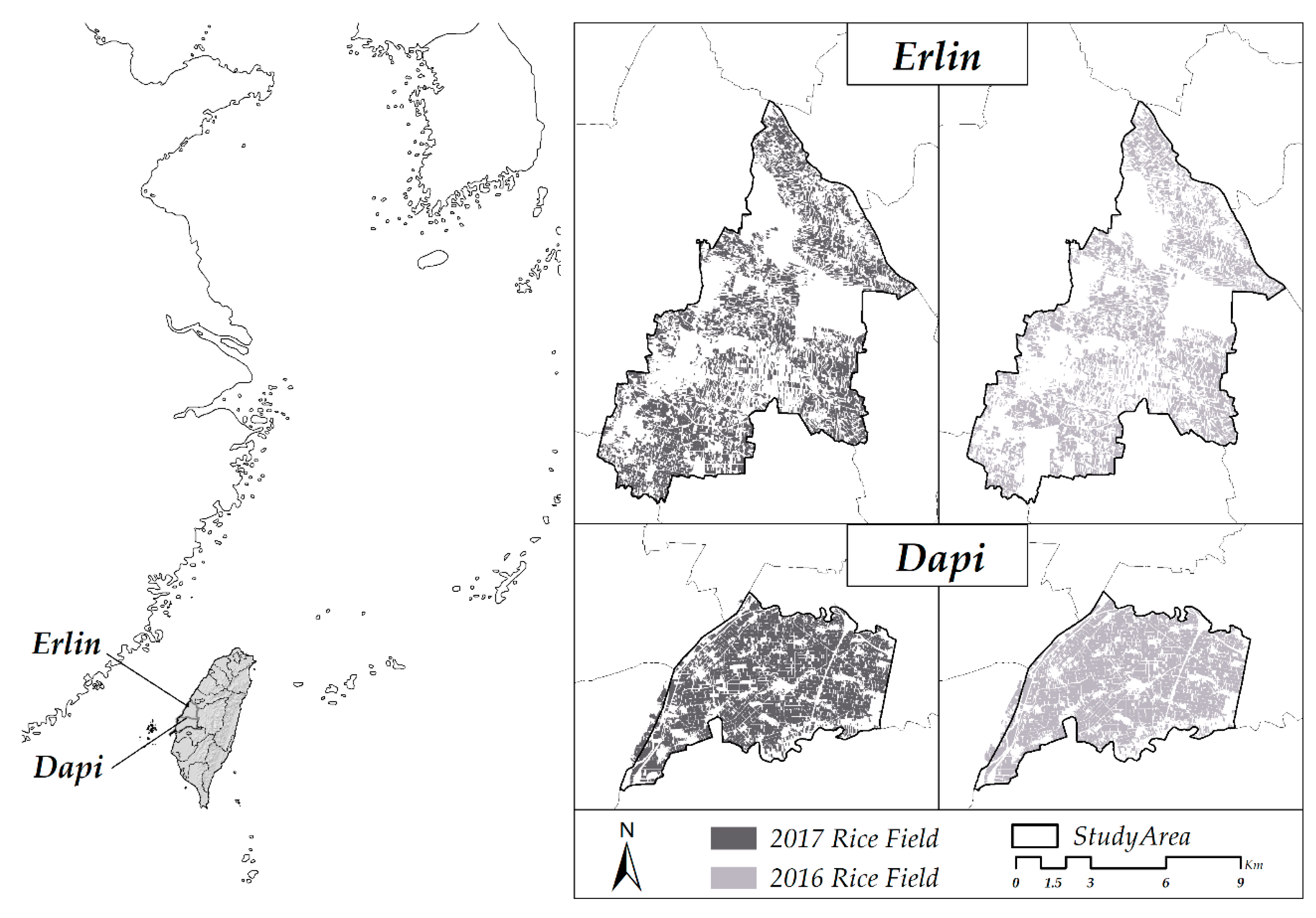
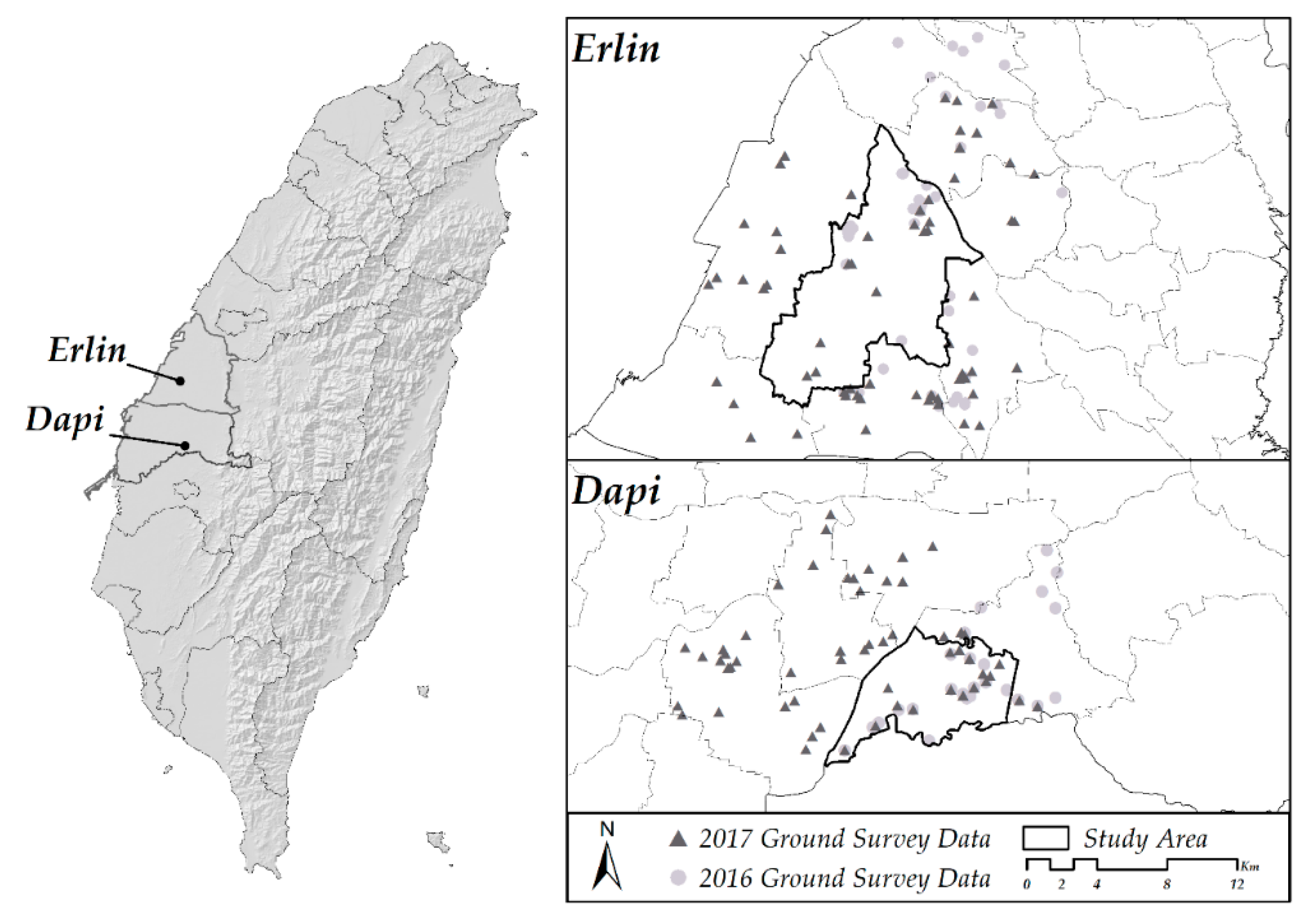
We chose Erlin in Changhua County, located in the latitude and longitude ranges of 23.855–23.999 N and 120.342–120.470 E, and Dapi in Yunlin County, located in the ranges of 23.609–23.680 N and 120.365–120.476 E, as the study areas (Figure 1). Both of the two areas are located in west-central Taiwan and serve as key agricultural production areas. The rainy season is mainly May through September, and the drought period is October through January [78]. The starting dates of the most active tillering stages in these two areas are slightly different. Paddy rice grows faster in Dapi because the weather is warmer and more humid. In 2016, the area of all of the rice fields in Erlin and Dapi was 3075.02 ha and 2856.92 ha, respectively; in 2017 the area was 3372.78 ha and 2767.09 ha, respectively.

2.3. Image and Yield Data Acquistion

The following principles were applied in image selection so as to diminish interference from the images toward the estimation of the rice yield. Firstly, the imagery that was not affected by cloud cover or cloud shadow was preferred; secondly, the date of the captured images was close to the harvest date. However, because the optical satellite imagery was subject to differences in weather, acquisition time, and region, the dates of the images used in the study are shown in

Table 4. Descriptive statistics of the yields in the ground survey samples and the actual total yields in the Erlin and Dapi townships.

	Year	Date of SPOT 1	Num.	Max. (t. ha−1)	Min. (t. ha−1)	Aver. (t. ha−1)	Std. (t. ha−1)	Proportion to All Rice Fields	Actual Total Yield (ton)
Erlin	2016	19/05/2016	40	8.473	6.462	7.500	0.583	0.514%	21.882.4
	2017	07/05/2017	63	10.205	6.347	7.858	0.709	0.655%	24.661.3
Dapi	2016	28/03/2016	26	11.530	4.864	8.230	1.393	0.242%	21.311.2
	2017	07/05/2017	57	9.679	3.726	8.127	1.036	0.547%	22.232.1

¹ Note: dd/mm/yyyy.

.

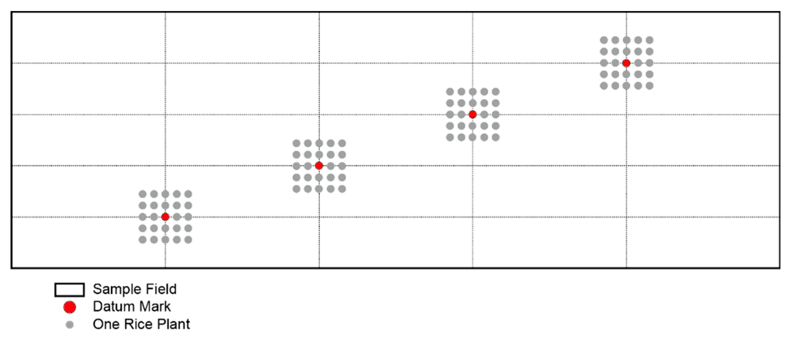
The yield data used in this study contained ground survey data and total yield data. As for the ground survey data, the Agriculture and Food Agency [79] uses sample data to survey the per-unit rice yield in Taiwan; these data include an orthophoto base map, a map of result of the investigated land use, and rice field distribution maps, which systematically extract sample fields. The data of the ground survey were collected and compiled from hand sampling. Four datum marks are selected from the sample field as the basis for estimating the rice yield of the current year. The sampling method commonly used in Taiwan is shown in Figure 2. For one given sample field, the collection area for each datum mark is around 1.2 m × 1.2 m, including 25 rice plants (the gray dots illustrates in Figure 2); where a total of 100 rice plants were collected and weigh measured, and the average weight per unit section (t. ha⁻¹) for this given sample field was calculated at well. The average weight of the rice per unit section was regarded as the dependent variable in this study, to build up the regression models.

Because the ground survey data were limited in Erlin and Dapi in 2016 and 2017, this study combined the ground survey data along with the surrounding area in Changhua and Yulin County, respectively, as the dependent variable. After the removal of the ground survey data affected by cloud shadow and cloud cover in the acquired SPOT images, the number and the spatial distribution of the ground survey data for the analysis are illustrated in Table 4 and Figure 3, respectively.

Because of the data acquisition limitation, the yield data for each paddy rice land parcel is not available. Therefore, we used the total yield data as the substitute for the model validation and error rate calculation. The total yield data acquired from the official statistical reports were published by AFA, which provides the yield data for each township in Taiwan by each cultivation period. The total yield data was counted by summing up the investigation results, which were provided by each township office after the harvest season of paddy rice at the end of the cultivation period. Therefore, in this study, we called these data the actual total yield data (Table 4).

2.4. Regression Models

OLS, SVR, and GWR were used to build the yield estimation models. The following is a brief description of SVR and GWR.

SVM was originally used for the classification problems, and SVR was applied for linear regression. Converting a nonlinear data space into a higher dimensional kernel feature space through nonlinear mapping accurately predicts the plane of the data distribution, and addresses the ever-present prediction problems.

ŷ_i = f(x_i,w) = ϕT(x_i)w + b

(1)

where ŷ_i represents the estimation of y_i, w is a weight vector in the feature space, and b is the bias term in the regression. The kernel function is usually used to switch the transition function T(x_i) in order to avoid the complex high-dimension calculation. In this study, we choose a nonlinear radial basis function (RBF) to build the yield estimation models.

The uniform distribution in geospatial space is hindered by the regional variation, and commonly used linear or nonlinear regression models were used to cover the local spatial characteristics because of the model hypothesis. To accurately explore the spatial attributes, Brunsdon et al. (1996) proposed a GWR model. According to the neighboring relationships and the spatial attributes of the spatial units, weights were established for the individual features, and regression calculations were performed between their own spatial units and the neighboring units. This method is commonly used to analyze the marginal effect of x on y, caused by the differences in geospatial space.

GWR4 was developed and programmed by Professor Tomoki Nakaya from Ritsumeikan University, Kyoto, Japan. The main purpose of GWR4 is to provide fitting GWR models, including conventional Gaussian models, Poisson models, and logistic regression models. The present study adopted Gaussian models. According to the geographic (fixed or adaptive) and kernel function (Gaussian or bi-square), four kernel types are available in GWR4. With a fixed kernel and constant local coefficients, the local extent of the adaptive kernels is controlled by the kth nearest neighboring distances for each regression location. Because the ground survey data were extracted from the sample field through systematic sampling, where the ground survey data were uniformly distributed, we tended to use the bi-square of the kernel functions. In addition to the criteria described previously, we used Akaike’s Information Criterion corrected for small sample size (AICc) as the selection criterion.

$$Y_i={\beta }_0(u_i,v_i)+{\beta }_i(u_i,v_i)X_i+{\epsilon }_i$$

(2)

$$\beta ={(X^{T}WX)}^{-1}{X}^{T}WX$$

(3)

where $Y_i$ and $X_i$ are the dependent and independent variables, respectively; $(u_i,v_i)$ represents the x and y coordinates of location I, respectively; $\beta$ is the coefficient of the $(u_i,v_i)$ location; ${\epsilon }_i$ is the error term; and $W$ is the spatial weights matrix. The fixed bi-square kernel used in this study is as follows:

$$w_{ij}=\{\begin{array}{cc}{(1-d_{ij}^2/{\theta }^2)}^2& d_{ij}<\theta \\ 0& d_{ij}>\theta \end{array}$$

(4)

where $w_{ij}$ is the weight value of the observation at location j for estimating the coefficient at location I, $d_{ij}$ is the Euclidean distance between i and j, and $\theta$ is a fixed bandwidth size defined by a distance metric measure.

The OLS model, nonlinear SVR model, and linear spatial econometrics GWR model were used in this study. Multiple statistical models were utilized to build and apply a yield estimation model. Based on an OLS model, this study compared nonlinear SVR, which has a multidimensional feature space, and the linear spatial econometrics GWR, which builds the weight for each grid, so as to determine which statistical model is more suitable for estimating the rice yield.

2.5. Constructing the Yield Estimation Model

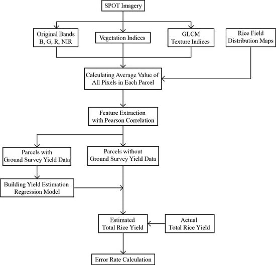
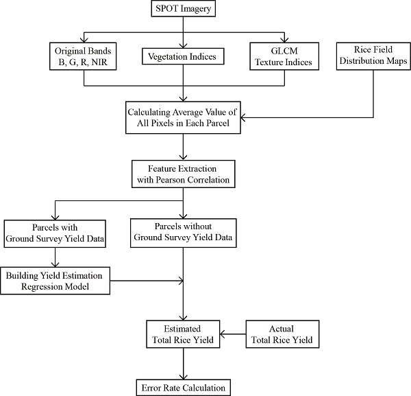
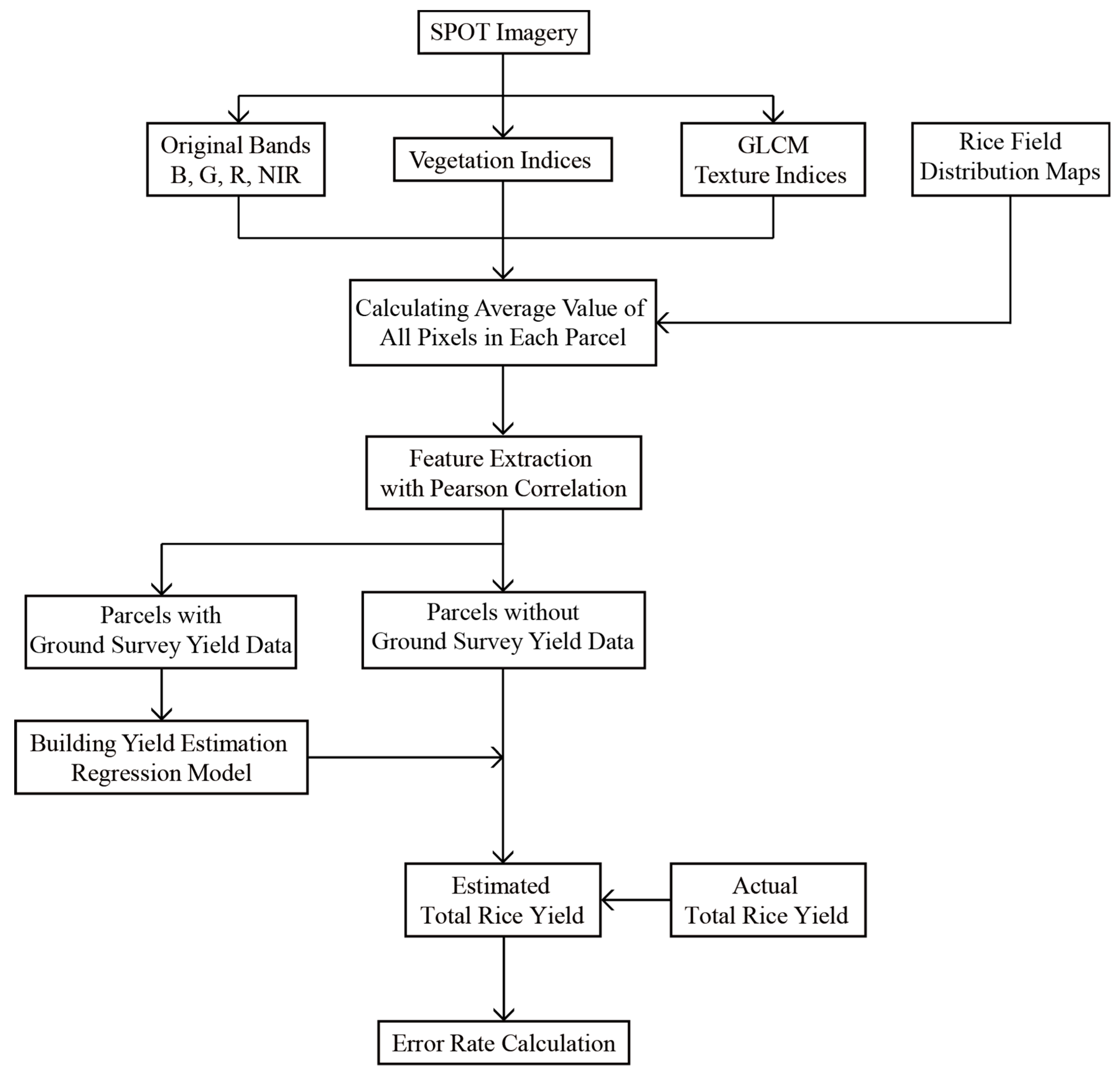
A detailed flowchart is shown in Figure 4. This study conducted its analysis by using OLS, SVR, and GWR. On account of the small number of ground survey data samples, this study used the actual rice yield of the ground survey data as the dependent variable, and four original (blue, green, red, and near-infrared) bands in the satellite imagery, as well as the spectral information and textural information, as the independent variables. The adjusted R² applied the verifying and further explaining power and error rate of the model.

The original bands, spectral information, and GLCM texture indices were extracted from the first-cultivation ground survey data in 2016 and 2017, from Erling and Dapi, along with the surrounding area in Changhua and Yunlin County, which served as the dependent variable. To avoid the influence of extreme values, we extracted the average value of all of the pixels in the ground survey data. After estimating the total rice yield, we calculated the error rate (ER) with actual total data and the following equation:

$$ER=\frac{P_{est}-P_{real}}{P_{real}}\times 100\%$$

(5)

where P_est is the estimated rice yield and P_real is the actual total data.

3. Results

Table 5. Rice yield estimation in the first cultivations of 2016 and 2017 in Erlin. OLS—ordinary least squares; SVR—support vector regression; GWR—geographically weighted regression (GWR).

Year	Combination	Selected Variable	OLS	SVR	GWR
2016	1	47	−6.50%	5.42%	F 2
	2	B, G, R, NIR, GI, MSAVI, NDVI, RVI, SecR 1	−2.59%	6.31%	7.46%
	3	B, MSAVI, RVI, SecR	−2.53%	6.31%	−2.47%
2017	1	47	5.13%	7.16%	F
	2	G, NIR, GI, RVI, TSAVI, HomG, VarR, VarNIR	6.96%	6.84%	6.91%
	3	G, NIR, GI, RVI, TSAVI, VarR	6.87%	6.64%	6.80%

Note: ¹ The GLCM variable name with the suffix R represents that this GLCM variable is derived from the red band; and suffixes B, G, and NIR represent blue, green, and near-infrared bands, respectively. ² F represents the estimation failed in the given regression model and combination.

illustrates the results by summarizing the data from the estimation of the rice yield in Erlin in 2016 and 2017. The percentage in Table 5 is the error rate (ER) calculated using Equation (5). Among the 2016 first-cultivation yield estimations of the three yield estimation models, the results of the rice yield were most unfavorable for the Combination 1 model, and the GWR model could not even be calculated. The rice yield error rates of the OLS model and SVR model were −6.50% and 5.42%, respectively. In Combinations 2 and 3, the SVR rice yield errors were no different, and the OLS model error was reduced through the process of feature selection. As for the results of the GWR rice yield, the errors were quite different when compared with the combinations. The rice yield error result of Combination 3 was the best result for 2016; the error was −2.47%.

For the first-cultivation yield estimation of 2017, the OLS model was most accurate when Combination 1 was used; the rice yield error was 5.13%. The GWR model could not be calculated for 2017. In Combination 2, the rice yield errors were similar among all three of the models; the same result was also observed for Combination 3.

A comparison of the rice yield errors in Erlin revealed that the rice yield errors of 2016 and 2017 were stable with SVR, but the accuracy was not optimal. The OLS model was unstable. Through the process of feature selection, the rice yield accuracy using the GWR model improved.

For the estimation of the rice yield in the first cultivations of 2016 and 2017 in Dapi, images were taken in 28 March 2016 and 7 May 2017. Compared with the images used from Erlin, the image acquisition time for Dapi in 2016 was closer to the appearance of the transplanting time, and that in 2017 was affected by the cloud cover and cloud shadow. Therefore, the estimation error for the rice yield in both years in Dapi was more severe than that in Erlin.

Regarding the 2016 first-cultivation yield estimation for Dapi in Yunlin County, all of the rice yield errors were close to 12% (

Table 6. Rice yield estimation in the first cultivations of 2016 and 2017 in Dapi.

Year	Combination	Selected Variable	OLS	SVR	GWR
2016	1	47	−10.35%	11.34%	F
	2	B, G, R, NIR, GI, MSAVI, RVI, SAVI, VarNIR	11.07%	11.34%	10.34%
	3	B, NIR, GI, SAVI, VarNIR	10.91%	13.22%	10.32%
2017	1	47	−3.64%	2.78%	F
	2	B, R, MSAVI, SAVI, CorNIR, DisNIR, EntNIR, HomNIR, MeaNIR	−1.47%	3.20%	−1.81%
	3	B, GI, MSAVI, SAVI, EntNIR, MeaNIR	−1.79%	2.75%	0.06%

). In Combination 1, the rice yield error of the nonlinear SVR model was 11.34%, and the GWR model could not be calculated. In Combination 2, the rice yield errors with the GWR model were the smallest among the three yield estimation models; the error was 10.34%. This result for Combination 2 was also observed for Combination 3; the GWR model was the best of the three yield estimation models, with an error of 10.32%. The rice yield error of OLS shifted greatly from underestimation to overestimation. Specifically, SVR with feature selection engendered a large yield estimation error.

A comparison of the overall estimation error values of Dapi revealed that according to the analysis results of the rice production in 2016 and 2017, whether the accuracy of OLS and SVR could be improved through the screening of variables could not be determined. Additionally, the acquisition date in the first cultivation was 28 March 2016, which was close to the appearance of the transplanting time. This was inconsistent with the dates in the first cultivations in 2016 and 2017 between Erlin and Dapi. It was speculated that this was the cause of the severe error in rice yield.

In order to increase the number of training samples and considering the spatial and temporal variation for the regression models, we also tried to combine the ground survey samples from different locations and years (hereafter referred to as mixed samples). Taking Combination 1 as an example, the error of OLS and SVR in the same year, in 2017, was −3.64% and 2.78%, respectively, and the error rate with the mixed samples became −2.00% and −0.33%, respectively. The error rate of Combinations 2 and 3 in Dapi were also reduced. Even if it is estimated through mixed samples, the error of estimation is much more likely to be larger. Conversely, if the area with less estimation error in the same year is estimated with mixed samples, it is possible to reduce the estimation error. As

Table 7. Rice yield estimation for 2017 in the first cultivations with mixed ground survey data from Erlin and Dapi in 2016 and 2017.

Area	Combination	Selected Variable	OLS	SVR	GWR
Erlin	1	47	6.36%	9.39%	F
	2	B, R, CMFI, GI, CorN, EntNIR, HomNIR, MeaNIR	7.84%	8.68%	6.31%
	3	B, GI, HomNIR, MeaNIR	7.71%	10.69%	3.89%
Dapi	1	47	−2.00%	−0.33%	F
	2	B, R, CMFI, GI, CorN, EntNIR, HomNIR, MeaNIR	−1.11%	1.16%	−0.81%
	3	B, GI, HomNIR, MeaNIR	−0.98%	1.84%	−1.03%

show, compared to the OLS and SVR results, the GWR estimation results are relatively stable, and most of the error rates are reduced by using mixed samples. The error rates of Combinations 2 and 3 in Erlin in 2017 were 6.91% and 6.80%, but the error rates decreased to 6.31% and 3.89% with the mixed samples. Although the results in Dapi were not obviously improved with the mixed samples, the error rates were all below 2%.

4. Discussion

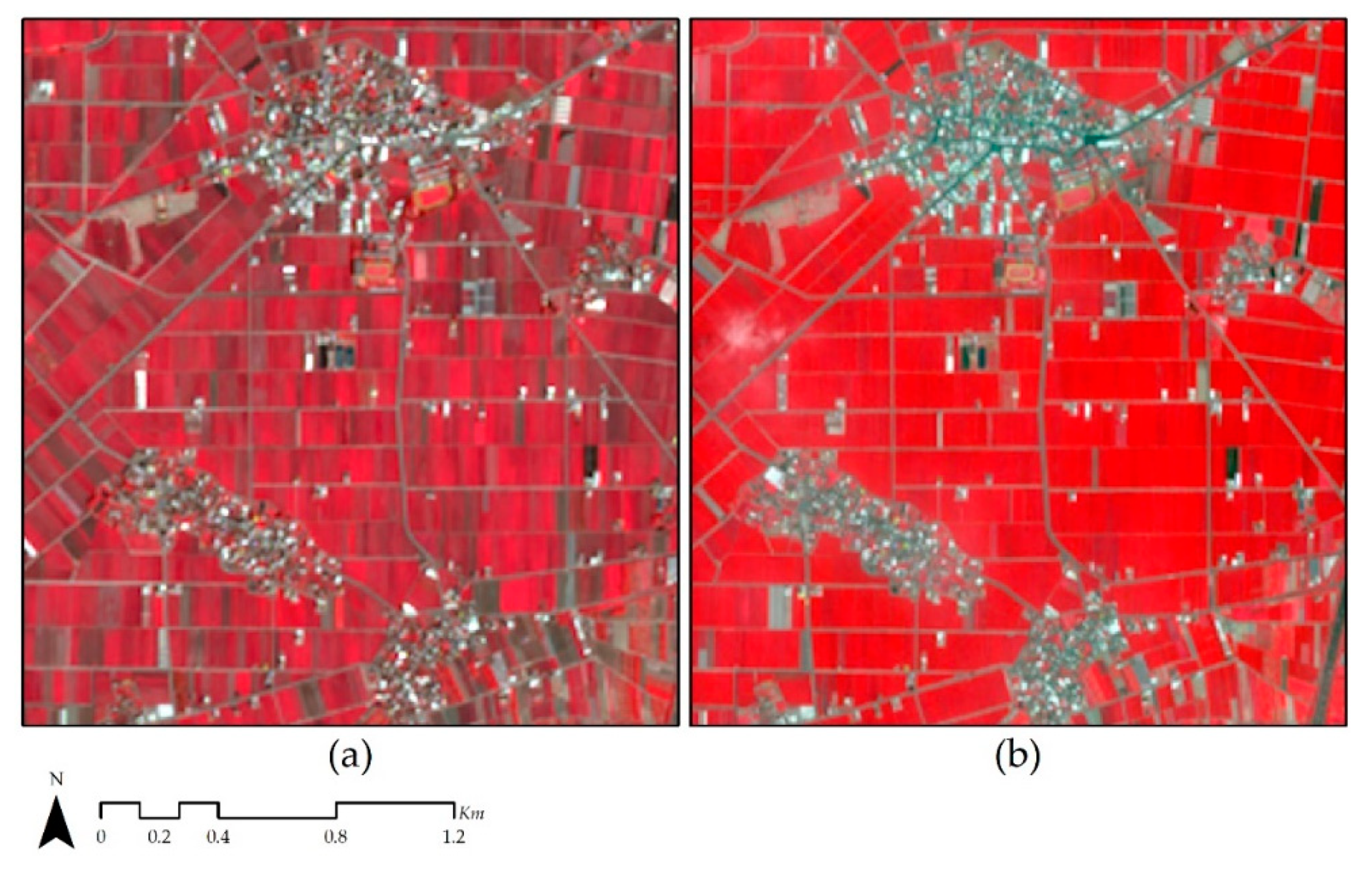
Overall, in the results of rice yield estimation in the first cultivations of 2016 and 2017, the rice yield error values were high, and the estimated yields were unstable in the OLS and nonlinear SVR models. We believe that problems such as spatial autocorrelation and spatial heterogeneity may not be considered and result in the poor accuracy of SVR production estimation. The rice yield error of Dapi in 2016 was evidently significant; it was speculated that the image acquisition date was close to the appearance of the transplanting time. According to the website of the TDARES, the first cultivation’s rice seedlings of mid–late maturity rice in central Taiwan is from the end of February to the beginning of March. The image of Dapi on 28 March 2016 was compared with the image on 7 May 2017 in the same area. Figure 5 show that some fields still did not present a spectral vegetation pattern. A comparison of the SPOT-7 images and the actual ground survey data distribution showed that the transplanting times in the first cultivation in Dapi were relatively consistent and synchronized; furthermore, making mistakes in image classification was difficult. The results showed that the transplanting times were more consistent, which was more favorable for rice yield estimation.

Through feature selection for Erlin, the error of the first-cultivation rice yield in the OLS model slightly underestimated the yield in 2016; however, in 2017, the yield was overestimated. With the nonlinear SVR model for yield estimation, the error in the rice yield estimation of the first cultivation in 2016 increased, whereas it was noticed that a slight decrement in 2017 slightly decreased. When the first-cultivation rice yield of 2016 and 2017 in Dapi was estimated through OLS, the error was marginally reduced. The SVR model estimate error of Combination 2 was higher than those toward the other variable combinations.

Through feature selection, Combinations 2 and 3 were estimated using the GWR model, and the rice yield error was lower than the number in Combination 1. The GWR model performed relatively steadily, the number of variables still needed to be considered when it was being conducted by GWR though. In this study, the 47 variables of Combination 1 failed to estimate the yield with the GWR model; this may infer the importance of feature selection before the input of independent variables to the GWR model.

To sum up all of the experiments from Table 6 and Table 7, we found that the original blue, green, and red bands, along with MSAVI, RVI, and near-infrared derivative GLCM Hom and Var indices, were selected more frequently than the other variables for rice yield estimation in both of the study areas and years. Therefore, we thought that these variables would be the key factors for yield estimation. As for the limitations of three regression models, OLS is constructed from linear variables and tries to find a regression line with the smallest residual. It can be completed quickly in the calculation process. However, in most of the studies, it cannot be explained by linear regression, it will be adjusted by the situation of the study. Second, SVR applies SVM to the discussion of the regression calculation, and finds the minimum distance of all of the observation samples to the hyperplane. Because SVR belongs to nonlinear model, the fitting effect is better. However, the parameter setting plays an important role in the calculation process. If the setting is slightly wrong, over-fitting or under-fitting will occur [80]. The above two calculation methods are based on the overall situation, but the regional problems cannot be considered. Therefore, in this study, GWR is used to consider the regional issues. GWR considers the case of spatial variability. According to the first law of geography, the distance has an obvious influence on the observation points, and the neighboring relationship and spatial attributes are used to establish different weights [81]. From the actual situation, it can be found that the yield production is obviously related to the regional factors. Therefore, when GWR is applied to observe the rice yield, the regional factors should be properly considered.

5. Conclusions

Most studies using optical satellite imagery cannot obtain identical conditions, including location, acquisition time, and cloud cover, all of which affect the study results. The first cultivation’s rice seedlings for mid–late maturity rice in central Taiwan are found between the end of February and late June. Because the yield estimation in the first cultivation in Dapi in 2016 could be achieved only using SPOT-7 on 28 March 2016, the date was evidently close to the appearance of the transplanting time; this caused a large error in the rice yield.

Overall, for the rice cultivation rice yield estimates for Erlin and Dapi, the results of the GWR model were the most suitable. The feature selection revealed that for 2016 and 2017 in Erlin, which was not affected by the date of image capture or cloud cover, the estimation errors were −2.47% and 6.80%, respectively. The image data of the rice yield for the first cultivation in Dapi were affected by cloud cover, but the error values were −1.81% and 0.06%, which were the lowest errors in this study.

In this study, OLS, nonlinear SVR, and linear spatial econometrics GWR models were used to build and apply a yield estimation model. The SVR model builds a hyperplane of higher dimensional feature space, whereas the GWR model considers the spatial distribution problem, corrects spatial autocorrelation and spatial heterogeneity, and adds the concept of a marginal effect. Where the GWR model establishes different weight values for spatial grids, the OLS and nonlinear SVR models lack this feature; this led to the rice yield estimation of GWR in this study outperforming those of the other two models.

The ground survey data were difficult to obtain. In addition, the cultivation of the sample fields and the cooperation of farmers are not necessarily the same every year. Therefore, because of the spatial autocorrelation and heterogeneity observed in this study, in future research, we intend to estimate the rice yield in different regions or in the same regions in the same period, by using ground survey data to reduce the instability of such data or several samples of such data.

References

- Food and Agriculture Organization (FAO). FAOSTAT Statistics Database; Food and Agriculture Organization of the United Nations: Rome, Italy, 2018. [Google Scholar]
- Prasad, A.K.; Chai, L.; Singh, R.P.; Kafatos, M. Crop yield estimation model for Iowa using remote sensing and surface parameters. Int. J. Appl. Earth Obs. Geoinf. 2006, 8, 26–33. [Google Scholar] [CrossRef]
- Chen, C.; Quilang, E.J.P.; Alosnos, E.D.; Finnigan, J. Rice area mapping, yield, and production forecast for the province of Nueva Ecija using RADARSAT imagery. Can. J. Remote Sens. 2011, 37, 1–16. [Google Scholar] [CrossRef]
- Prasad, A.; Singh, R.; Tare, V.; Kafatos, M. Use of vegetation index and meteorological parameters for the prediction of crop yield in India. Int. J. Remote Sens. 2007, 28, 5207–5235. [Google Scholar] [CrossRef]
- Sarma, A.; Kumar, T.L.; Koteswararao, K. Development of an agroclimatic model for the estimation of rice yield. J. Ind. Geophys. Union 2008, 12, 89–96. [Google Scholar]
- Savin, I.Y.; Isaev, V. Rice yield forecast based on satellite and meteorological data. Russ. Agric. Sci. 2010, 36, 424–427. [Google Scholar] [CrossRef]
- Teoh, C.; Nadzim, N.M.; Shahmihaizan, M.M.; Izani, I.M.K.; Faizal, K.; Shukry, H.M. Rice yield estimation using below cloud remote sensing images acquired by unmanned airborne vehicle system. Int. J. Adv. Sci. Eng. Inf. Technol. 2016, 6, 516–519. [Google Scholar] [CrossRef]
- Patel, N.; Ravi, N.; Navalgund, R.; Dash, R.; Das, K.; Patnaik, S. Estimation of rice yield using IRS-1A digital data in coastal tract of Orissa. Remote Sens. 1991, 12, 2259–2266. [Google Scholar] [CrossRef]
- Zhou, X.; Zheng, H.; Xu, X.; He, J.; Ge, X.; Yao, X.; Cheng, T.; Zhu, Y.; Cao, W.; Tian, Y. Predicting grain yield in rice using multi-temporal vegetation indices from UAV-based multispectral and digital imagery. ISPRS J. Photogram. Remote Sens. 2017, 130, 246–255. [Google Scholar] [CrossRef]
- Swain, K.C.; Thomson, S.J.; Jayasuriya, H.P. Adoption of an unmanned helicopter for low-altitude remote sensing to estimate yield and total biomass of a rice crop. Trans. ASABE 2010, 53, 21–27. [Google Scholar] [CrossRef]
- Mabalay, M.; Quilang, E.; Nelson, A.; Setiyono, T.; Maunahan, A.; Abonete, P.; Rola, A.; Raviz, J.; Skorzus, K.; Loro, J. Rice area mapping and yield estimation for crop insurance in Leyte Province [Philippines]. Philipp. J. Crop Sci. (Philippines) 2014, 39, 16. [Google Scholar]
- Noureldin, N.; Aboelghar, M.; Saudy, H.; Ali, A. Rice yield forecasting models using satellite imagery in Egypt. Egypt. J. Remote Sens. Space Sci. 2013, 16, 125–131. [Google Scholar] [CrossRef] [Green Version]
- Guo, J.; Wang, Q.; Zheng, T.; Li, X.; Shi, J.; Zhu, J. Estimation of rice yield based on integration remote sensing information and crop model. In Proceedings of the Remote Sensing and Modeling of Ecosystems for Sustainability IX, San Diego, CA, USA, 24 October 2012; p. 10. [Google Scholar]
- Son, N.; Chen, C.; Chen, C.; Minh, V.; Trung, N. A comparative analysis of multitemporal MODIS EVI and NDVI data for large-scale rice yield estimation. Agric. For. Meteorol. 2014, 197, 52–64. [Google Scholar] [CrossRef]
- Campos-Taberner, M.; García-Haro, F.; Camps-Valls, G.; Grau-Muedra, G.; Nutini, F.; Busetto, L.; Katsantonis, D.; Stavrakoudis, D.; Minakou, C.; Gatti, L. Exploitation of SAR and optical Sentinel data to detect rice crop and estimate seasonal dynamics of leaf area index. Remote Sens. 2017, 9, 248. [Google Scholar] [CrossRef]
- Mosleh, M.K.; Hassan, Q.K.; Chowdhury, E.H. Application of remote sensors in mapping rice area and forecasting its production: A review. Sensors 2015, 15, 769–791. [Google Scholar] [CrossRef] [PubMed]
- Lasko, K.; Vadrevu, K.P.; Tran, V.T.; Justice, C. Mapping Double and Single Crop Paddy Rice With Sentinel-1A at Varying Spatial Scales and Polarizations in Hanoi, Vietnam. IEEE J. Sel. Top. Appl. Earth Obs. Remote Sens. 2018, 11, 498–512. [Google Scholar] [CrossRef] [PubMed]
- Mansaray, L.R.; Huang, W.; Zhang, D.; Huang, J.; Li, J. Mapping rice fields in urban Shanghai, Southeast China, using Sentinel-1A and Landsat 8 datasets. Remote Sens. 2017, 9, 257. [Google Scholar] [CrossRef]
- Lee, S.-K.; Yoon, S.; Won, J.-S. Vegetation Height Estimate in Rice Fields Using Single Polarization TanDEM-X Science Phase Data. Remote Sens. 2018, 10, 1702. [Google Scholar] [CrossRef]
- Zhang, Y.; Liu, X.; Su, S.; Wang, C. Retrieving canopy height and density of paddy rice from Radarsat-2 images with a canopy scattering model. Int. J. Appl. Earth Obs. Geoinf. 2014, 28, 170–180. [Google Scholar] [CrossRef]
- Shao, Y.; Fan, X.; Liu, H.; Xiao, J.; Ross, S.; Brisco, B.; Brown, R.; Staples, G. Rice monitoring and production estimation using multitemporal RADARSAT. Remote Sens. Environ. 2001, 76, 310–325. [Google Scholar] [CrossRef]
- Maki, M.; Sekiguchi, K.; Homma, K.; Hirooka, Y.; Oki, K. Estimation of rice yield by SIMRIW-RS, a model that integrates remote sensing data into a crop growth model. J. Agric. Meteorol. 2017, 73, 2–8. [Google Scholar] [CrossRef] [Green Version]
- Setiyono, T.; Holecz, F.; Khan, N.; Barbieri, M.; Quicho, E.; Collivignarelli, F.; Maunahan, A.; Gatti, L.; Romuga, G. Synthetic Aperture Radar (SAR)-based paddy rice monitoring system: Development and application in key rice producing areas in Tropical Asia. IOP Conf. Ser. Earth Environ. Sci. 2017, 54, 012015. [Google Scholar] [CrossRef] [Green Version]
- Li, Y.; Liao, Q.; Li, X.; Liao, S.; Chi, G.; Peng, S. Towards an operational system for regional-scale rice yield estimation using a time-series of Radarsat ScanSAR images. Int. J. Remote Sens. 2003, 24, 4207–4220. [Google Scholar] [CrossRef]
- Chen, C.; McNairn, H. A neural network integrated approach for rice crop monitoring. Int. J. Remote Sens. 2006, 27, 1367–1393. [Google Scholar] [CrossRef]
- Setiyono, T.D.; Quicho, E.D.; Gatti, L.; Campos-Taberner, M.; Busetto, L.; Collivignarelli, F.; García-Haro, F.J.; Boschetti, M.; Khan, N.I.; Holecz, F. Spatial rice yield estimation based on MODIS and Sentinel-1 SAR data and ORYZA crop growth model. Remote Sens. 2018, 10, 293. [Google Scholar] [CrossRef]
- Horie, T.; Nakagawa, H.; Centeno, H.; Kropff, M. The rice crop simulation model SIMRIW and its testing. Model. Impact Clim. Chang. Rice Prod. Asia 1995, 4, 51–66. [Google Scholar]
- Zhang, S.; Tao, F.; Shi, R. Modeling the rice phenology and production in China with SIMRIW: Sensitivity analysis and parameter estimation. Front. Earth Sci. 2014, 8, 505–511. [Google Scholar] [CrossRef]
- Homma, K.; Maki, M.; Hirooka, Y. Development of a rice simulation model for remote-sensing (SIMRIW-RS). J. Agric. Meteorol. 2017, 73, 9–15. [Google Scholar] [CrossRef] [Green Version]
- Benkedjouh, T.; Medjaher, K.; Zerhouni, N.; Rechak, S. Health assessment and life prediction of cutting tools based on support vector regression. J. Intell. Manuf. 2015, 26, 213–223. [Google Scholar] [CrossRef]
- Hamdi, T.; Ali, J.B.; Di Costanzo, V.; Fnaiech, F.; Moreau, E.; Ginoux, J.-M. Accurate prediction of continuous blood glucose based on support vector regression and differential evolution algorithm. Biocybern. Biomed. Eng. 2018, 38, 362–372. [Google Scholar] [CrossRef]
- Zhang, F.; Deb, C.; Lee, S.E.; Yang, J.; Shah, K.W. Time series forecasting for building energy consumption using weighted Support Vector Regression with differential evolution optimization technique. Energy Build. 2016, 126, 94–103. [Google Scholar] [CrossRef]
- Chen, K.; Yu, J. Short-term wind speed prediction using an unscented Kalman filter based state-space support vector regression approach. Appl. Energy 2014, 113, 690–705. [Google Scholar] [CrossRef]
- Jiang, H.; Zhang, Y.; Muljadi, E.; Zhang, J.J.; Gao, D.W. A short-term and high-resolution distribution system load forecasting approach using support vector regression with hybrid parameters optimization. IEEE Trans. Smart Grid 2018, 9, 3341–3350. [Google Scholar] [CrossRef]
- Wu, C.-H.; Ho, J.-M.; Lee, D.-T. Travel-time prediction with support vector regression. IEEE Trans. Intell. Transp. Syst. 2004, 5, 276–281. [Google Scholar] [CrossRef]
- Marković, N.; Milinković, S.; Tikhonov, K.S.; Schonfeld, P. Analyzing passenger train arrival delays with support vector regression. Transp. Res. Part C Emerg. Technol. 2015, 56, 251–262. [Google Scholar] [CrossRef]
- Chen, T.; Lu, S. Accurate and Efficient Traffic Sign Detection Using Discriminative AdaBoost and Support Vector Regression. IEEE Trans. Veh. Technol. 2016, 65, 4006–4015. [Google Scholar] [CrossRef]
- Were, K.; Bui, D.T.; Dick, Ø.B.; Singh, B.R. A comparative assessment of support vector regression, artificial neural networks, and random forests for predicting and mapping soil organic carbon stocks across an Afromontane landscape. Ecol. Indic. 2015, 52, 394–403. [Google Scholar] [CrossRef]
- Bui, D.T.; Tuan, T.A.; Klempe, H.; Pradhan, B.; Revhaug, I. Spatial prediction models for shallow landslide hazards: A comparative assessment of the efficacy of support vector machines, artificial neural networks, kernel logistic regression, and logistic model tree. Landslides 2016, 13, 361–378. [Google Scholar]
- Tien Bui, D.; Shahabi, H.; Shirzadi, A.; Chapi, K.; Alizadeh, M.; Chen, W.; Mohammadi, A.; Ahmad, B.; Panahi, M.; Hong, H. Landslide detection and susceptibility mapping by AIRSAR data using support vector machine and index of entropy models in Cameron Highlands, Malaysia. Remote Sens. 2018, 10, 1527. [Google Scholar] [CrossRef]
- Oguntunde, P.G.; Lischeid, G.; Dietrich, O. Relationship between rice yield and climate variables in southwest Nigeria using multiple linear regression and support vector machine analysis. Int. J. Biometeorol. 2018, 62, 459–469. [Google Scholar] [CrossRef]
- Yuan, H.; Yang, G.; Li, C.; Wang, Y.; Liu, J.; Yu, H.; Feng, H.; Xu, B.; Zhao, X.; Yang, X. Retrieving soybean leaf area index from unmanned aerial vehicle hyperspectral remote sensing: Analysis of RF, ANN, and SVM regression models. Remote Sens. 2017, 9, 309. [Google Scholar] [CrossRef]
- Son, N.-T.; Chen, C.-F.; Chen, C.-R.; Minh, V.-Q. Assessment of Sentinel-1A data for rice crop classification using random forests and support vector machines. Geocarto Int. 2018, 33, 587–601. [Google Scholar] [CrossRef]
- Ndikumana, E.; Minh, D.H.T.; Thu, D.N.H.; Baghdadi, N.; Courault, D.; Hossard, L.; El Moussawi, I. Rice height and biomass estimations using multitemporal SAR Sentinel-1: Camargue case study. In Proceedings of the Remote Sensing for Agriculture, Ecosystems, and Hydrology XX, Berlin, Germany, 10 October 2018. [Google Scholar]
- Imran, M.; Stein, A.; Zurita-Milla, R. Using geographically weighted regression kriging for crop yield mapping in West Africa. Int. J. Geogr. Inf. Sci. 2015, 29, 234–257. [Google Scholar] [CrossRef]
- Haghighattalab, A.; Crain, J.; Mondal, S.; Rutkoski, J.; Singh, R.P.; Poland, J. Application of geographically weighted regression to improve grain yield prediction from unmanned aerial system imagery. Crop Sci. 2017, 57, 2478–2489. [Google Scholar] [CrossRef]
- Cai, R.; Yu, D.; Oppenheimer, M. Estimating the spatially varying responses of corn yields to weather variations using geographically weighted panel regression. J. Agric. Resour. Econ. 2014, 230–252. [Google Scholar]
- Kerry, R.; Goovaerts, P.; Giménez, D.; Oudemans, P. Investigating temporal and spatial patterns of cranberry yield in New Jersey fields. Precis. Agric. 2017, 18, 507–524. [Google Scholar] [CrossRef]
- Caetano, J.M.; Tessarolo, G.; de Oliveira, G.; e Souza, K.d.S.; Diniz-Filho, J.A.F.; Nabout, J.C. Geographical patterns in climate and agricultural technology drive soybean productivity in Brazil. PLoS ONE 2018, 13, e0191273. [Google Scholar] [CrossRef]
- Bitter, C.; Mulligan, G.F.; Dall’erba, S. Incorporating spatial variation in housing attribute prices: A comparison of geographically weighted regression and the spatial expansion method. J. Geogr. Syst. 2007, 9, 7–27. [Google Scholar] [CrossRef]
- Huang, Y.; Leung, Y. Analysing regional industrialisation in Jiangsu province using geographically weighted regression. J. Geogr. Syst. 2002, 4, 233–249. [Google Scholar] [CrossRef]
- Dziauddin, M.F.; Powe, N.; Alvanides, S. Estimating the effects of light rail transit (LRT) system on residential property values using geographically weighted regression (GWR). Appl. Spat. Anal. Policy 2015, 8, 1–25. [Google Scholar] [CrossRef]
- Murakami, T.; Nakajima, S.; Takahashi, T.; Nishihara, Y.; Imai, A.; Kikushima, R.; Sato, T. Spatially Varying Impacts of Farmers Markets on Agricultural Land Use. 2014. Available online: https:// https://ssrn.com/abstract=245071 (accessed on 31 October 2018).
- Kimsey Jr, M.J.; Moore, J.; McDaniel, P. A geographically weighted regression analysis of Douglas-fir site index in north central Idaho. For. Sci. 2008, 54, 356–366. [Google Scholar]
- Windle, M.J.; Rose, G.A.; Devillers, R.; Fortin, M.-J. Exploring spatial non-stationarity of fisheries survey data using geographically weighted regression (GWR): An example from the Northwest Atlantic. ICES J. Mar. Sci. 2009, 67, 145–154. [Google Scholar] [CrossRef]
- Osborne, P.E.; Foody, G.M.; Suárez-Seoane, S. Non-stationarity and local approaches to modelling the distributions of wildlife. Divers. Distrib. 2007, 13, 313–323. [Google Scholar] [CrossRef]
- Víquez-R, L.R.; Arias-Alzate, A.; Ceballos, G. Spatial patterns of species richness and functional diversity in Costa Rican terrestrial mammals: Implications for. Divers. Res. 2015, 22, 43–56. [Google Scholar]
- Propastin, P. Modifying geographically weighted regression for estimating aboveground biomass in tropical rainforests by multispectral remote sensing data. Int. J. Appl. Earth Obs. Geoinf. 2012, 18, 82–90. [Google Scholar] [CrossRef]
- Propastin, P.; Kappas, M.; Erasmi, S. Application of Geographically Weighted Regression to Investigate the Impact of Scale on Prediction Uncertainty by Modelling Relationship between Vegetation and Climate. IJSDIR 2008, 3, 73–94. [Google Scholar]
- Sadorus, L.L.; Mantua, N.J.; Essington, T.; Hickey, B.; Hare, S. Distribution patterns of Pacific halibut (Hippoglossus stenolepis) in relation to environmental variables along the continental shelf waters of the US West Coast and southern British Columbia. Fish. Oceanogr. 2014, 23, 225–241. [Google Scholar] [CrossRef]
- Acharya, B.K.; Cao, C.; Lakes, T.; Chen, W.; Naeem, S.; Pandit, S. Modeling the spatially varying risk factors of dengue fever in Jhapa district, Nepal, using the semi-parametric geographically weighted regression model. Int. J. Biometeorol. 2018, 62, 1973–1986. [Google Scholar] [CrossRef]
- Huang, J.; Huang, Y.; Pontius, R.G.; Zhang, Z. Geographically weighted regression to measure spatial variations in correlations between water pollution versus land use in a coastal watershed. Ocean Coast. Manag. 2015, 103, 14–24. [Google Scholar] [CrossRef]
- Li, C.; Li, F.; Wu, Z.; Cheng, J. Exploring spatially varying and scale-dependent relationships between soil contamination and landscape patterns using geographically weighted regression. Appl. Geogr. 2017, 82, 101–114. [Google Scholar] [CrossRef]
- Chen, J.; Zhou, C.; Wang, S.; Hu, J. Identifying the socioeconomic determinants of population exposure to particulate matter (PM 2.5) in China using geographically weighted regression modeling. Environ. Pollut. 2018, 241, 494–503. [Google Scholar] [CrossRef]
- Wan, S.; Chang, S.-H.; Peng, C.-T.; Chen, Y.-K. A novel study of artificial bee colony with clustering technique on paddy rice image classification. Arab. J. Geosci. 2017, 10, 215. [Google Scholar] [CrossRef]
- Haboudane, D.; Miller, J.R.; Tremblay, N.; Zarco-Tejada, P.J.; Dextraze, L. Integrated narrow-band vegetation indices for prediction of crop chlorophyll content for application to precision agriculture. Remote Sens. Environ. 2002, 81, 416–426. [Google Scholar] [CrossRef]
- Rondeaux, G.; Steven, M.; Baret, F. Optimization of soil-adjusted vegetation indices. Remote Sens. Environ. 1996, 55, 95–107. [Google Scholar] [CrossRef]
- Jeong, S.; Ko, J.; Yeom, J.-M. Nationwide Projection of Rice Yield Using a Crop Model Integrated with Geostationary Satellite Imagery: A Case Study in South Korea. Remote Sens. 2018, 10, 1665. [Google Scholar] [CrossRef]
- Yang, J.; Du, L.; Gong, W.; Shi, S.; Sun, J.; Chen, B. Potential of vegetation indices combined with laser-induced fluorescence parameters for monitoring leaf nitrogen content in paddy rice. PLoS ONE 2018, 13, e0191068. [Google Scholar] [CrossRef] [PubMed]
- Yue, J.; Yang, G.; Li, C.; Li, Z.; Wang, Y.; Feng, H.; Xu, B. Estimation of winter wheat above-ground biomass using unmanned aerial vehicle-based snapshot hyperspectral sensor and crop height improved models. Remote Sens. 2017, 9, 708. [Google Scholar] [CrossRef]
- Wiegand, C.; Shibayama, M.; Yamagata, Y.; Akiyama, T. Spectral observations for estimating the growth and yield of rice. Jpn. J. Crop Sci. 1989, 58, 673–683. [Google Scholar] [CrossRef]
- Panda, S.S.; Ames, D.P.; Panigrahi, S. Application of vegetation indices for agricultural crop yield prediction using neural network techniques. Remote Sens. 2010, 2, 673–696. [Google Scholar] [CrossRef]
- Gilabert, M.A.; González-Piqueras, J.; Garcίa-Haro, F.J.; Meliá, J. A generalized soil-adjusted vegetation index. Remote Sens. Environ. 2002, 82, 303–310. [Google Scholar] [CrossRef] [Green Version]
- Cutler, M.; Boyd, D.; Foody, G.; Vetrivel, A. Estimating tropical forest biomass with a combination of SAR image texture and Landsat TM data: An assessment of predictions between regions. ISPRS J. Photogram. Remote Sens. 2012, 70, 66–77. [Google Scholar] [CrossRef] [Green Version]
- Charoenjit, K.; Zuddas, P.; Allemand, P.; Pattanakiat, S.; Pachana, K. Estimation of biomass and carbon stock in Para rubber plantations using object-based classification from Thaichote satellite data in Eastern Thailand. J. Appl. Remote Sens. 2015, 9, 096072. [Google Scholar] [CrossRef] [Green Version]
- Zheng, H.; Cheng, T.; Zhou, M.; Li, D.; Yao, X.; Tian, Y.; Cao, W.; Zhu, Y. Improved estimation of rice aboveground biomass combining textural and spectral analysis of UAV imagery. Precis. Agric. 2018. [Google Scholar] [CrossRef]
- Yamamoto, K.; Guo, W.; Yoshioka, Y.; Ninomiya, S. On plant detection of intact tomato fruits using image analysis and machine learning methods. Sensors 2014, 14, 12191–12206. [Google Scholar] [CrossRef] [PubMed]
- Central Weather Bureau Observation Data Inquire System. Available online: https://e-service.cwb.gov.tw/HistoryDataQuery/index.jsp (accessed on 31 October 2018).
- Nuarsa, I.W.; Nishio, F.; Hongo, C. Rice yield estimation using Landsat ETM+ data and field observation. J. Agric. Sci. 2011, 4, 45. [Google Scholar] [CrossRef]
- Chang, Q.; Chen, Q.; Wang, X. Scaling Gaussian RBF kernel width to improve SVM classification. In Proceedings of the International Conference on Neural Networks and Brain, Beijing, China, 13–15 October 2005; pp. 19–22. [Google Scholar]
- Brunsdon, C.; Fotheringham, A.S.; Charlton, M.E. Geographically weighted regression: A method for exploring spatial nonstationarity. Geogr. Anal. 1996, 28, 281–298. [Google Scholar] [CrossRef]
Figure 1.
Study area and rice field distribution maps.
Figure 2.
Schematic of ground survey data collection method commonly used in Taiwan.
Figure 3.
Ground survey data’s distribution maps for Erlin and Dapi.
Figure 4.
Flow chart of rice yield estimation. B—blue; R—red; G—green; NIR—near-infrared; GLCM—grey-level co-occurrence matrix.
Figure 5.
The first cultivation of Dapi in 2016 (a) and 2017 (b) with G, R, and NIR bands. The red areas on the images are all rice fields, but in 2016, they are a different color shade, which means that the transplanting time is not consistent, which influences the accuracy of the yield estimation.