Visible and Near-Infrared Reflectance Spectroscopy Analysis of a Coastal Soil Chronosequence
by
 , ,
, ,
Guanghui Zheng
1,2,3,* ,
,
Dongryeol Ryu
3 ,
,
Caixia Jiao
1,2,3,
Xianli Xie
4,
Xuefeng Cui
2,5 and
Gang Shang
1 1
School of Geographic Sciences, Nanjing University of Information Science & Technology, Nanjing 210044, China
2
Meteorology and Climate Centre, School of Mathematics and Statistics, University College Dublin, Belfield, Dublin 4, Ireland
3
Department of Infrastructure Engineering, University of Melbourne, Parkville 3010, Australia
4
Institute of Soil Science, Chinese Academy of Science, Nanjing 210008, China
5
School of Systems Science, Beijing Normal University, Beijing 100875, China
*
Author to whom correspondence should be addressed.
Remote Sens. 2019, 11(20), 2336; https://doi.org/10.3390/rs11202336
Submission received: 4 September 2019
/
Revised: 4 October 2019
/
Accepted: 7 October 2019
/
Published: 9 October 2019
(This article belongs to the Special Issue Estimation and Mapping of Soil Properties Based on Multi-Source Data Fusion)
Abstract
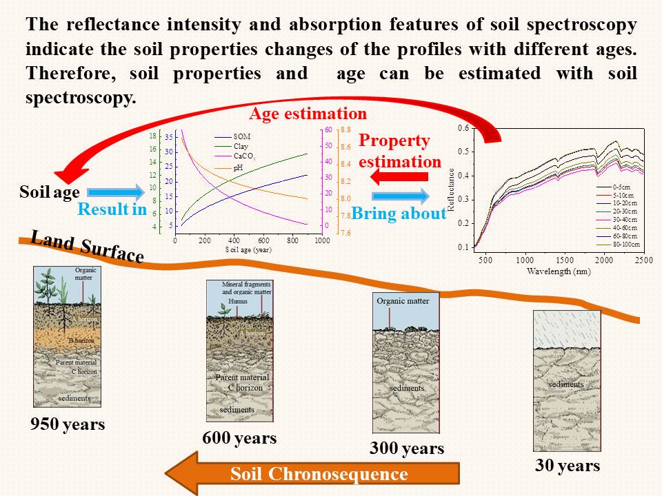
:The soil chronosequence is a useful method for investigating pedological theories. Soil chemical, physical and mineralogical properties in chronosequences change over time and exhibit systematic and time-dependent trends, which can be used to analyze the rates and directions of pedogenic changes. The potential of soil spectroscopy as an emerging, rapid and cost-effective technique for predicting soil properties has been widely accepted and has motivated the application of spectroscopic techniques to the analysis of soil chronosequence. We present a soil chronosequence derived from 1000-year-old calcareous marine sediments and examine changes in six soil properties over this period. We evaluated the utility of a soil spectroscopic method to detect soil property changes and to predict the pedogenic properties and soil ages of the chronosequence. The results show that some soil pedogenic processes, such as soil organic matter accumulation, CaCO3 leaching and clay migration, can be identified in the millennium chronosequence. Power chronofunctions are formulated for soil organic matter (SOM) and Logarithmic chronofunctions are fitted for clay, CaCO3 and pH. These pedogenic processes are identified in the reflectance intensity and absorption features of soil spectroscopy, and pedogenic properties can be calibrated via soil reflectance spectroscopy. Profile ages can also be predicted via pseudo multi-depth spectra of soil profiles, and soil spectral curves for 0–30 cm generated the best prediction results (RPD = 1.85). We conclude that soil properties, changing due to weathering and soil formation, act as a bridge linking spectroscopy and weathering levels/pedogenic processes. The results imply that applying spectroscopy techniques to chronosequence study and mapping the degree of soil development in certain areas should be possible.

1. Introduction
According to soil genesis theory, soil is a natural body formed through the synthetic actions of parent materials, climate, topography, organisms, and time [1]. These factors continuously determine changes in soil-forming processes, resulting in soil evolution [2]. Every soil profile records its genetic process, developmental history and duration of its exposure to soil-forming factors [3]. A series of soil profiles, developed based on similar soil-forming factors with the exception of time, consist of a soil chronosequence [2] which splices brief segments of the soil evolution history [4]. Consequently, spatial difference between the soil profiles can be translated into temporal differences [5]. Therefore, soil chronosequences can reveal the rates and directions of pedogenic changes and provide invaluable information for examining pedogenic theories and processes [5,6]. Soil properties in a chronosequence exhibit systematic and time-dependent features, i.e., soil organic matter (SOM) [7,8], iron oxide [9,10], clay minerals [11], particle size distribution [12], and CaCO3 [13,14]. These properties are also called pedogenic properties. Therefore, these time-dependent pedogenic properties can be used for relative age dating [15]. Furthermore, chronofunctions of soil properties were developed to determine the stage and the rates of soil development, and to ascertain the time of reaching steady state [16].
The chemical and physical properties are conventionally measured through laboratory-based “wet chemistry” analyses, which are costly and time-consuming, and not suitable for rapid soil property mapping at multiple spatial scales. Whereas, considerable demand for high-quality and inexpensive soil data for environmental monitoring, modeling and precision agriculture requires more efficient and cost-effective methods of soil analysis nowadays [17]. Since Bowers and Hanks [18] and Condit [19] systematically investigated the relationship between soil properties and reflectance spectroscopy, the potential of soil spectroscopy as an efficient and cost-effective prediction technique has been demonstrated by a large number of subsequent studies [20,21,22,23]. This technique was also used in pedogenic research to explore the relationship between the degree of soil weathering and reflectance spectroscopy [24,25,26,27]. Demattê and Terra [28] investigated the reflectance of weathered soils in a toposequence and noted that soil changes, produced by different weathering levels or pedogenic processes, reflected spectral behaviors along the profile depth. Zheng et al. [29] concluded that the pedogenic properties provided a bridge between spectroscopy and the pedogenic processes, which makes it possible to analyze the chronosequence using spectroscopy. To the best of our knowledge, Awiti et al. [30] first evaluated the capability of spectroscopy to analyze soil property changes for topsoil (0–20 cm) across a forest-cropland chronosequence. However, a chronosequence that utilizes a series of deeper soil profiles with formation age, in addition to topsoils, may provide more comprehensive and accurate soil property changes and pedogenic processes.
The coastal soil is an important source of agricultural lands in China and the understanding of soil dynamics under long-term cultivation is critical to planning the sustainable use of the soil resource. Chen et al. [31] and Cui et al. [32] revealed the dynamic changes in soil properties through the chronosequence derived from the sediments of the Yangtze River. However, few investigations of the soil dynamics of chronosequence formed by the sediments of the Yellow and Yangtze Rivers over the past 1000 years have been published.
In this work, we analyze fairly uniform calcareous marine sediments with exact coastline change records in order to evaluate the utility of soil profiles’ spectra for a chronosequence. More specific objectives are (i) to establish a soil chronosequence derived from 1000-year-old calcareous marine sediments and investigate soil property changes over this period, (ii) to evaluate the potential for surface soil spectroscopy to detect soil property changes with time in a chronosequence, and (iii) to assess the feasibility of predicting soil profile age in this area using spectroscopy.
2. Materials and Methods
2.1. Study Area and Soil Formation
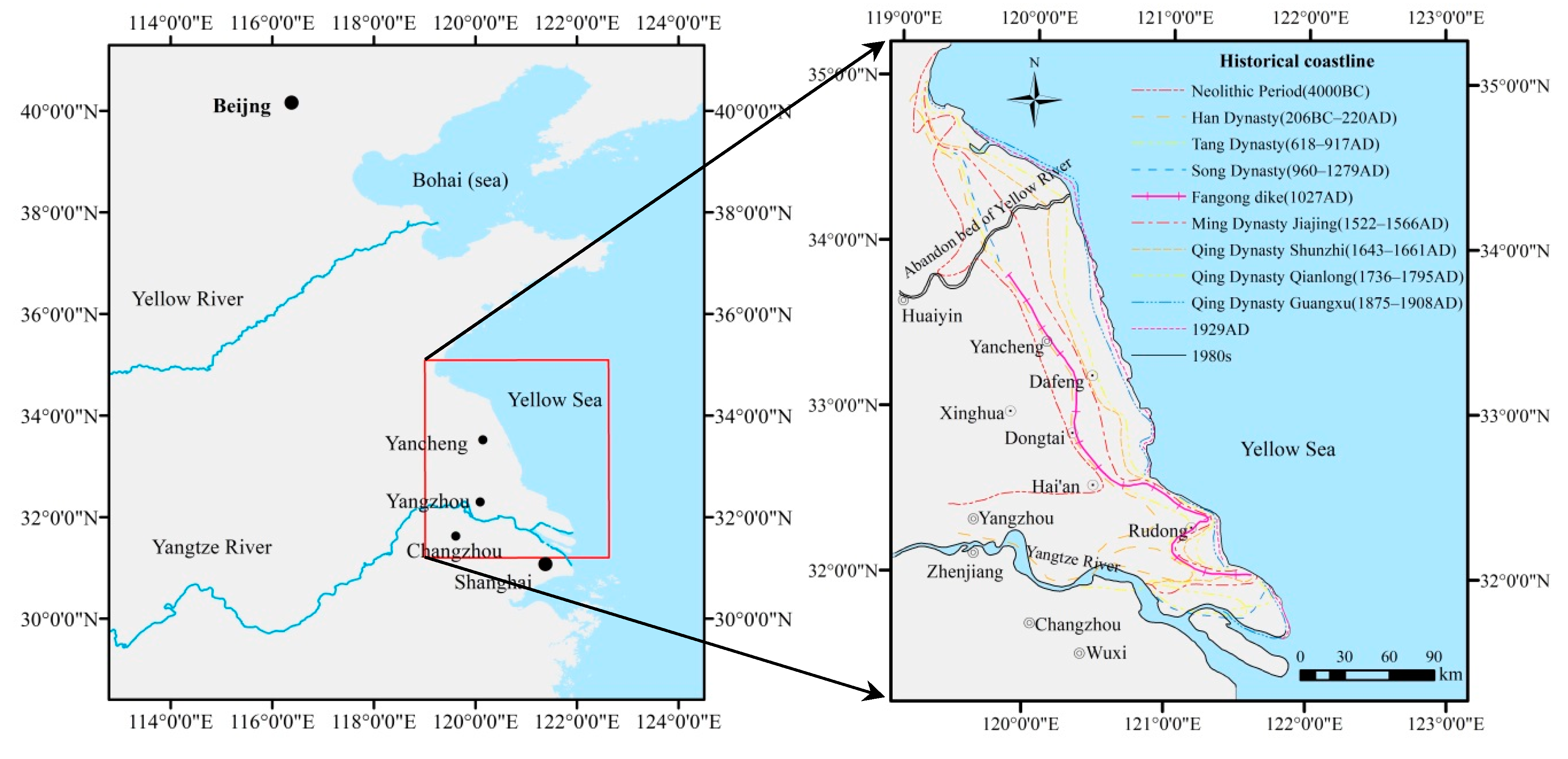
The study area is located in the coastal plain of Northern Jiangsu Province, China (Figure 1). The coastal plain east of the Fangong Dike, completed in 1027 AD, is formed of sediments transported mainly by the Yellow and the Yangtze Rivers over the past 1000 years. Historical changes of the coastline in Jiangsu Province are shown in Figure 1. This region is characterized by the northern subtropical monsoon climate. The mean annual precipitation and temperature are 1042.3 mm and 14.6 °C, respectively.
The soil formation and evolution in this area went through three stages. First, the seabeach, which was formed from sediments, evolved into a meadow solonchak (salt marsh) after the salt in the topsoil was leached out and salt-tolerant plants appeared. Secondly, SOM in the topsoil accumulated with the development of salt-tolerant plants, and soils further evolved into saline farming soils with the cultivation of salt-tolerant crops. Finally, dry-farming soils formed with the cultivation of corn– and rice–wheat/barley rotations.
2.2. Soil Sampling and Analysis
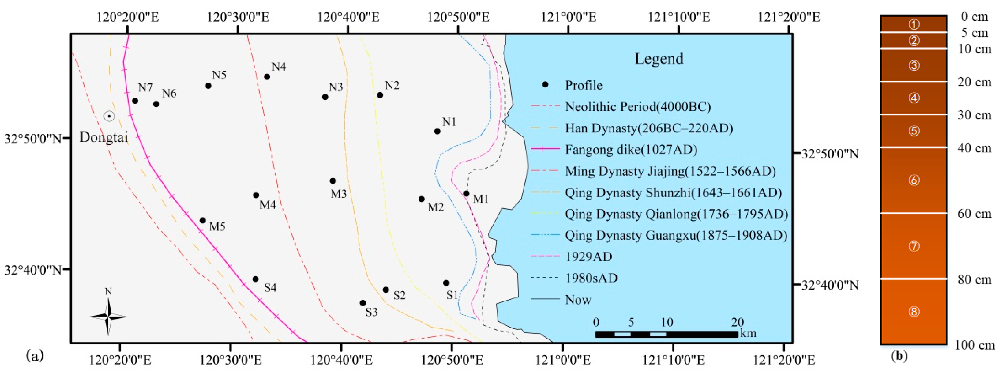
Sixteen soil sampling sites are located along three lines (north, middle and south) that generally run perpendicular to the coastlines (Figure 2a), and soil ages were estimated based on the historical coastlines to indicate the development degree of soil profiles [33]. The land use of all the sampling sites was farmland. All the soil profiles belong to the coastal saline alluvial soil, except profile S4, which is paddy soil according to Chinese Soil Genetic Classification System. To specify the soil property changes at various profile depths and compare the profile properties, the following sampling-depth intervals were used for each profile: 0–5, 5–10, 10–20, 20–30, 30–40, 40–60, 60–80 and 80–100 cm and 128 samples were collected. The samples for every specific depth interval were collected from the whole interval (Figure 2b) in June, 2013 and the weight for every sample is about 1–2 kg.
The soil samples were air-dried and gently crushed using a wooden pestle to pass through 2 mm nylon sieves. The subsamples were further ground using agate mortar and passed through 0.250 mm and 0.150 mm sieves to determine their physical and chemical properties. Soil pH was determined using the electrode method with a 1:5 (g:mL) ratio of soil and distilled water. SOM was measured by the potassium dichromate–external heating method, CaCO3 content was measured through neutralization titration, and the particle size distribution was determined using the pipette method. Total Fe (Fet) was determined by the HF-HNO3-HClO4 digestion–atomic absorption spectrophotometry method, free Fe oxides (Fed) were extracted using the dithionite-citrate-bicarbonate (DCB) method [34]. The descriptive statistics and correlation analysis of soil properties were performed by SPSS 20.0.
2.3. Spectra Determination
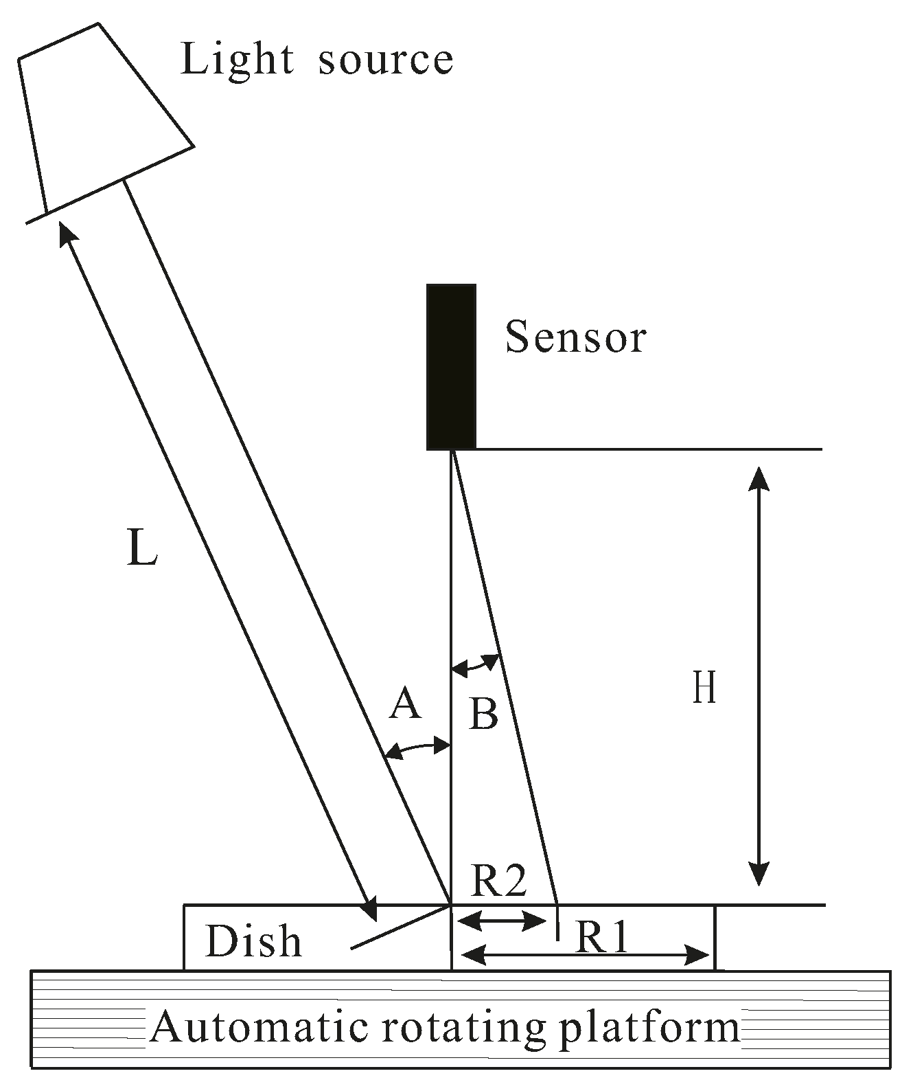
The air-dried soil samples passed through a 0.150 mm sieve were used for spectral measurements. Soil reflectance spectra were measured in a dark room with a FieldSpec 3 portable spectrometer (Analytical Spectral Devices Inc., Boulder, Colorado, USA). A 50 W halogen lamp set at a vertical angle of 15° (A) and at a distance 30 cm (L) from the samples was used as a light source. The sensor was vertically positioned 15 cm (H) above the soil samples using a probe set at a 5° viewing angle (half view angle B = 2.5°), producing a radius of 0.655 cm (R2) from the center of the sample dish (radius of sample dish R1 = 2.5 cm) (Figure 3). The dark current was removed prior to collecting the soil spectra, and a 40 cm × 40 cm diffuse reflection standard reference plate was used to obtain the relative reflectance. Throughout the measurement process, the soil sample in the container was rotated on an automatic rotating platform to average out the possible influence of different azimuth angles. Twenty spectral curves were collected for each sample as the sample was turned 360°. The reflectance spectrum for each sample was deemed the average of these 20 spectral curves.
2.4. Statistical Analysis and Transformation of the Spectral Data
Partial least squares regression (PLSR), first proposed by Wold et al. [35], is a commonly used modeling technique for calibrating soil properties to reflectance spectroscopy because it can resolve the issues of high collinearity among predictor variables (reflectance spectroscopy). PLSR integrates compression and regression steps and can effectively extract comprehensive variables (referred to as latent variables, LVs) by excluding unexplainable information, thus ensuring that comprehensive variables are optimally condensed from the raw inputs to explain response variables. Although various data-mining algorithms have been developed to determine soil properties using visible and near-infrared (VNIR) diffuse reflectance spectra and gave better performance than PLSR [36,37], the coefficients of PLSR can give the important wavelength to response variable which is useful to analyze the prediction mechanism. All calibration and prediction were performed by PLSR in Unscrambler X v. 10.0 (CAMO Software AS, Oslo, Norway). The data were centered before calibration and prediction automatically by checking the center data tick-boxes in this software. Full cross-validation was used for the cross-validation method in the calibration process. The optimal number of principal components was determined by the residual variance obtained in the unscrambler.
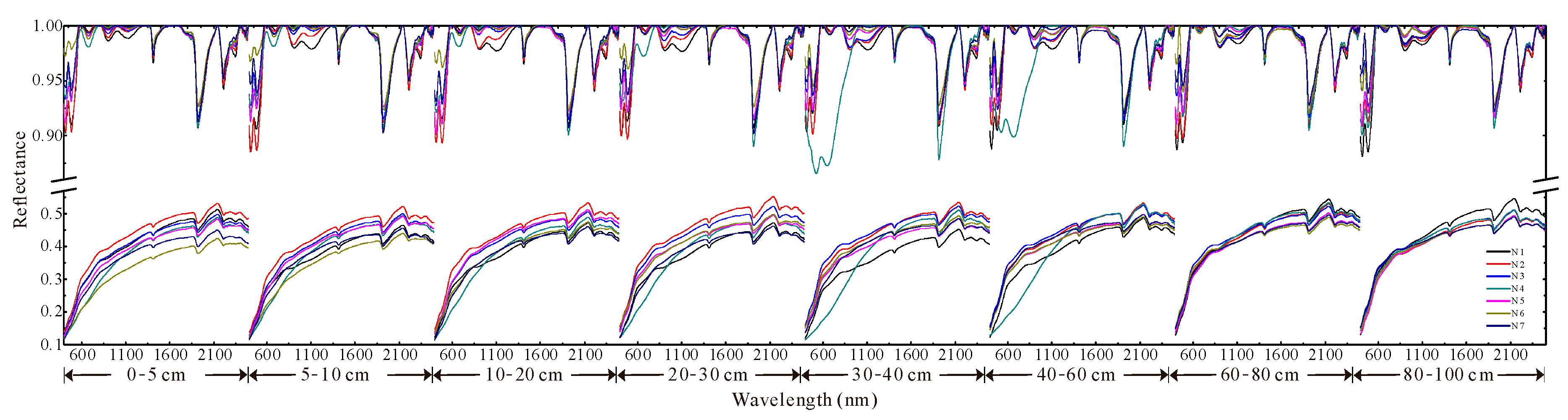
A continuum removal (CR) technique can be used to isolate particular absorption features for spectrum analysis and to define the band depth [38,39]. In this work, spectral curves were smoothed following Savitzky and Golay [40], with a second-order polynomial across 21 smoothing points using Unscrambler X v. 10.0 (CAMO Software AS, Oslo, Norway). These curves were then transformed via continuum removal in ENVI 4.7 (ITT Visual Information Solutions Inc., Broomfield, United States). For each soil profile, the smoothed and continuum-removed spectra from the eight depth intervals were joined in sequence to create a pseudo multi-depth soil spectral curve (Figure 4) according to Vasques et al. [41].
2.5. Datasets Partitioning and Accuracy Evaluating
All the samples were sorted according to profile number and depth in a profile. Four out of five samples were used for model development (calibration) and the others (one out of five) for model evaluation (prediction). The number of samples was 102 and 26 for the calibration and prediction (evaluation) sets, respectively.
Two principal components were extracted from the pseudo multi-depth curves of continuum-removed spectra of the sixteen profiles. Six profiles were selected for the prediction of soil age according to a scatter plot of two principal components and others were used for calibration of the profile age.
The model accuracies were evaluated using the coefficient of determination (R2, subscripts c for calibration, p for prediction) and residual prediction deviation (RPD). Viscarra Rossel et al. [17] classified RPD values into six classes: RPD < 1.0 indicates very poor results which are not recommended; RPD between 1.0 and 1.4 indicates poor results where only high and low values are distinguishable; RPD between 1.4 and 1.8 indicates fair results which may be used; RPD between 1.8 and 2.0 indicates good results where quantitative predictions are possible; RPD values between 2.0 and 2.5 indicate very good, quantitative model/predictions, and RPD > 2.5 indicates excellent model/predictions.
3. Results
3.1. Basic Statistics of Soil Properties
The descriptive statistics of soil properties are presented in Table 1. SOM were mainly distributed between 1.4 g kg−1 and 33.4 g kg−1 with a mean of 7.1 g kg−1, indicating a low SOM level in this area. Clay varied from 1.9% to 18.3% with a mean of 7.7% and a standard deviation of 4.0. CaCO3 ranged from 0.9 g kg−1 to 63.8 g kg−1 with a mean of 30.8 g kg−1. The value of pH varied from 6.4 to 9.2 with a mean of 8.5, indicating alkalinity because of CaCO3 in soil. Fed and Fed/Fet ranged from 1.8 g kg−1 to 6.6 g kg−1 and from 7.8% to 26.8%, respectively. SOM was the most variable property among these soil properties (CV = 86.9%), followed by CaCO3 (CV = 54.4%).
Table 2 lists the correlation coefficients of six soil properties. SOM had significant positive correlation with clay, while negative correlations with CaCO3 and pH. There were significant negative correlations between CaCO3 and clay, Fed and Fet, while there was a positive correlation with pH.
3.2. Soil Property Changes in Chronosequence and Pedogenic Interpretations
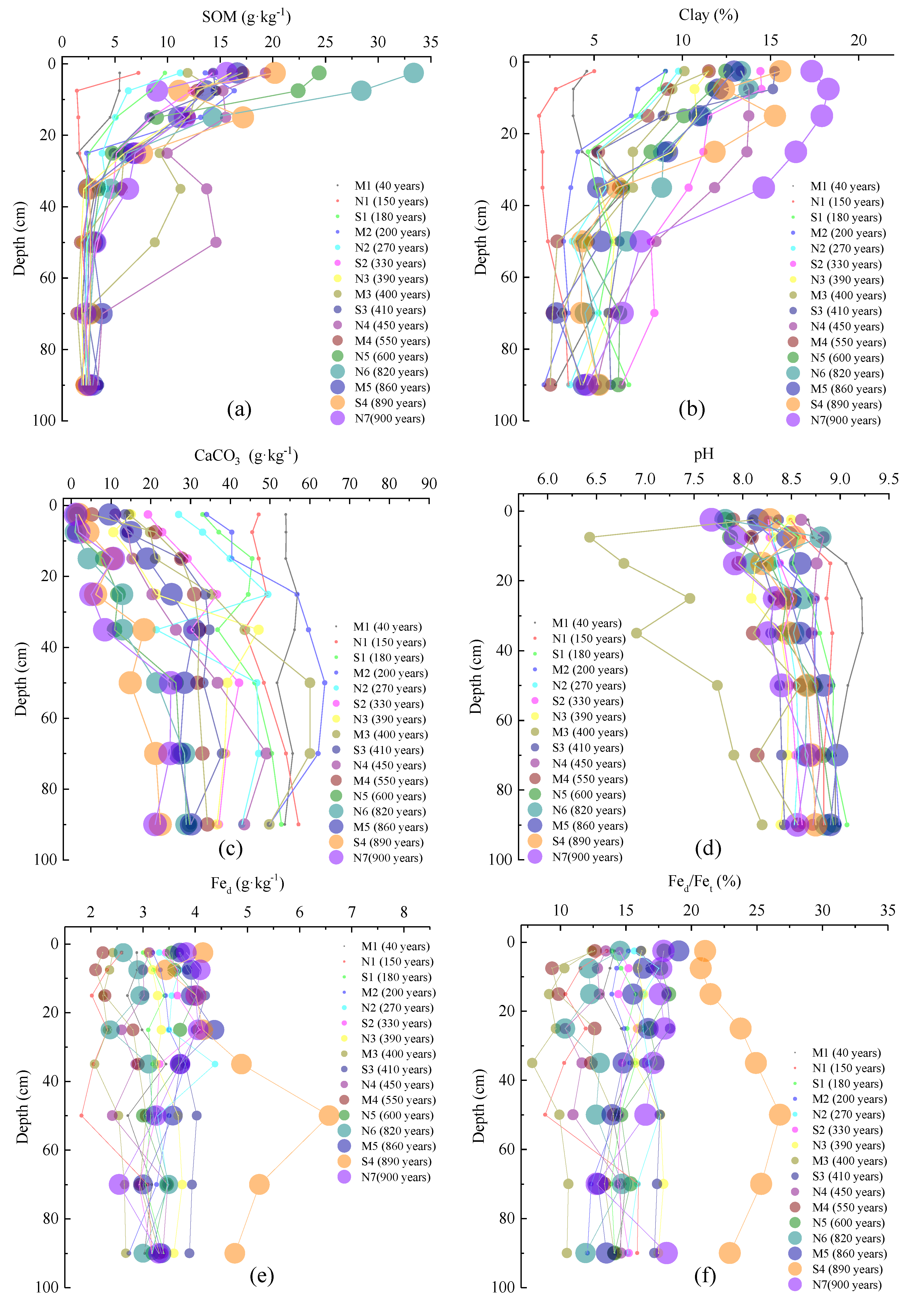
SOM, clay, pH, and CaCO3 exhibited direct dependences on age, and the vertical distribution of these properties changed regularly with depth (Figure 5). Trends over time and the vertical distribution of Fed were not evident. The changes in the properties in the top surface (0–5 cm) were fitted to analyze the chronofunctions. The four functions, including linear, power, exponential and logarithmic models, were used to fit the scatter, and the best fitted results were determined by the coefficients of determination and shown in Figure 6.
SOM increased with soil age between profiles and decreased with depth in a profile (Figure 5a). The vertical distribution of SOM in younger profiles (M1 and N1) is relatively uniform throughout the 0–100 cm soil depth. However, the differentiation in the vertical distribution of SOM in the profiles increased with soil age, i.e., older soils presented greater SOM differentiation between the topsoil and subsoil. In other words, the shapes of depth function of SOM changed gradually from uniform to exponential with soil age [42]. In addition, SOM was similar in the subsoil under a depth of 40 cm, except in the M3 and N4 profiles. The results suggested that SOM accumulation mainly occurred in the top 40 cm due to cultivation and biological activity of salt-tolerant plants. Brauer et al. [43] showed that paddy rice cultivation will lead to a dense plough pan and seriously reduces, but not totally prevents, downward transport of organic matter.
A scatter was plotted with SOM in the top soil sample (0–5 cm) as dependent and soil age as independent (Figure 6a). The functions, fitting to the scatter, were named chronofunctions, which were formulated relating the pedogenic properties to the ages of the soils [44]. A logarithmic model for SOM is common because it suggests that the SOM will approach a steady state [16]. However, power function got the best result (largest R2) among linear, logarithmic and power functions in this study (Figure 6a), which suggests that SOM in this area has not reached a steady state. The soil in this area can continue to play the role of carbon sequestration. This curve still displayed the general pattern of rapid increase in the first period and then a lower rate of accumulation [32,44,45]. The rate of SOM accumulation is different in many studies. Chen et al. [31] analyzed some studies about the time taken to reach a steady state and concluded that different environmental conditions may produce different response times. However, many studies proved that positive anthropogenic activities, especially rice–barley rotation and fertilization [6,7], will enhance the accumulation of SOC. Furthermore, the mass fraction of SOC was widely used for modeling chronofunction, but we think SOC density or stock is better for SOC accumulation analysis.
The changes in clay content were similar to those in SOM (Figure 5b). Clay content in the youngest profile was uniform, and differentiation between the topsoil and subsoil increased with age because larger particles physically and chemically weathered to smaller particle sizes over time [46,47]. The vertical distribution of clay content within a depth of 0–40 cm or less in every profile was more uniform than that of SOM, suggesting that clay migration and illuviation mainly occurred at this depth during the past 1000 years. Artificial irrigation and drainage during cultivation can favor clay accumulation and differentiation [48], which may be the cause of the difference of vertical distribution between clay and SOM. The total mass of accumulated clay is an excellent indicator of relative soil age during all stages of soil development [15]. However, the relationship between clay and age is different. Bockheim [49] concluded that the logarithmic model resulted in the best fit of clay in B horizon and Huang et al. [10] got the same result. However, VandenBygaart and Protz [44] indicated that a linear chronofunction was the best model to fit the increase in clay with soil age. In this study, logarithmic chronofunction obtained the best result (Figure 6b).
The CaCO3 content showed an inverse trend relative to SOM and clay. The CaCO3 contents were high and remained uniform in profile M1 and N1 and decreased with soil age due to leaching (Figure 5c), consistent with the results of previous studies [13,44]. A logarithmic curve fit to the scatter plot yielded a high determination coefficient (Figure 6c). In this study, high CaCO3 contents and rapid leaching rates appeared in the profiles of less than 600 years; low CaCO3 contents and lower leaching rates were found in the >600-year profiles in this study area. However, Chen et al. [31] found that CaCO3 was completely leached from paddy soil within a 300-year period. Wissing et al. [50] indicated that the upper 20 cm of soil was free of carbonates in 100-year-old paddy soils. Vidic and Lobnlk [13] discovered that carbonate clasts vanished from the upper horizons after 62 ka. Precipitation and the farming system of the study areas caused this difference, as precipitation (and resulting soil wetness) and vegetation type were the two main factors that affected the rate of carbonate weathering and the depth of leaching in carbonate-rich soils [44]. To the contrary, CaCO3 accumulation is the most characteristic age-related pedofeature in the semiarid regions where precipitation is insufficient [51]. The content of CaCO3 can be seen as an intrinsic threshold [52] because the changes in CaCO3 may be responsible for many successive processes. Firstly, the leaching of carbonates in soils is commonly a prerequisite to clay migration by eluviation. Secondly, Fed illuviation occurred only when carbonates were eventually leached because CaCO3 will retard the transformation of silicate Fe to Fe oxide [31]. There are significant negative correlations between CaCO3 and clay and Fed in this study (Table 2), which suggests that the leaching of CaCO3 is very important to clay and Fed.
Generally, the soil pH value decreased with soil age, following changes in the CaCO3 content (Figure 5d and Figure 6d). After about 1000 years of development, the soil pH decreased from >8.5 to nearly 7.5. The relationship between pH and CaCO3 is significant and positive (Table 2). Therefore, the best-fit curve of pH scatter was logarithmic, the same as that of CaCO3 (Figure 6d). There were significant negative relationships between pH and SOM and Clay (Table 2). Vidic and Lobnlk [13] demonstrated that carbonate leaching and the corresponding decrease in pH created favorable conditions for clay translocation.
In contrast with the above-listed properties, Fed and Fed/Fet did not exhibit evident trends correlated with soil age. The vertical distributions of these two properties were relatively uniform in each profile, compared with the above four properties (Figure 5e,f). The fitted chronofunctions of these two properties still showed positive linear relationships with soil age (Figure 6e,f). In general, Fed and Fed/Fet increased with age due to the irreversible transformation degree from primary iron silicate minerals to secondary iron oxide [32,53].
3.3. Spectroscopy Analysis of Top Soil
Soil spectroscopy is a cumulative property derived from the intrinsic spectral behavior of a heterogeneous combination of soil constituents [54]. SOM, clay minerals, carbonate, iron oxides, moisture, and particle size are important factors for reflectance [55]. These soil properties simultaneously determine the reflected energy [24] and form spectral curves. Therefore, changes in the soil properties can be studied based on diagnostic absorption features [56].
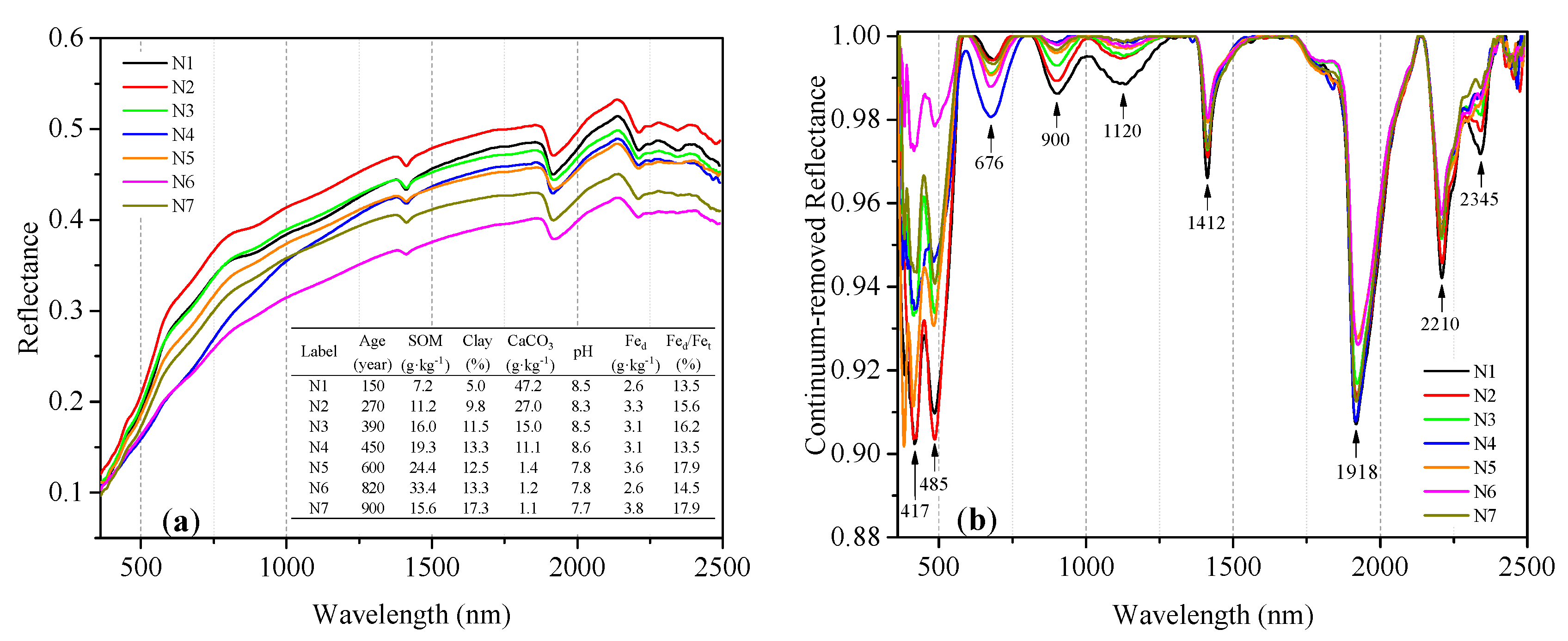
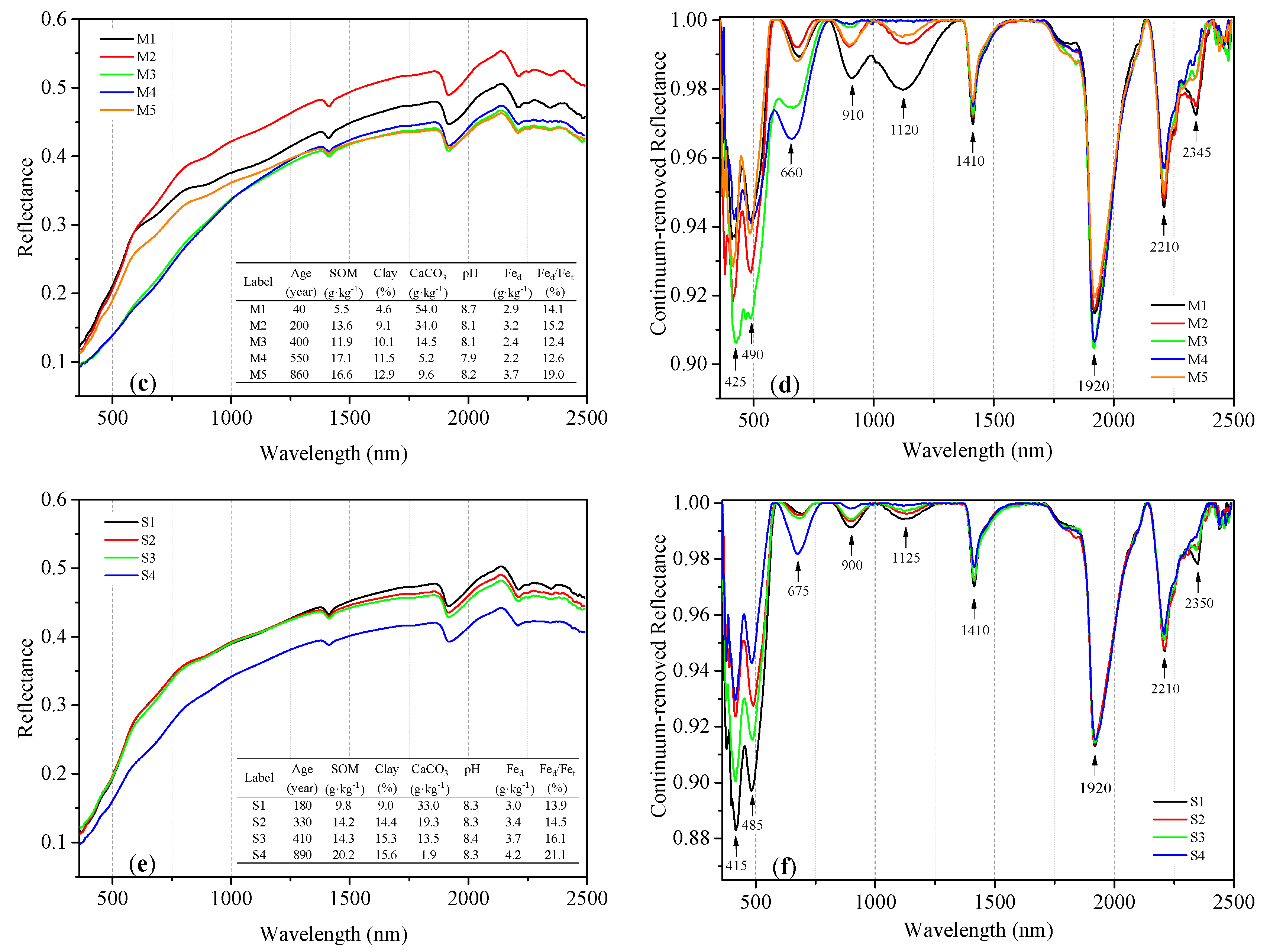
In order to describe the changes in the soil spectroscopy clearly, these profiles were divided into three groups, i.e., north line, middle line and south line, and each group is perpendicular to historical coastlines (Figure 2a). The original and continuum-removed spectral curves of topsoil were plotted in Figure 7. In the range of 350–1300 nm, the original reflectance density increased rapidly and the curves were convex with some broad absorption features by electronic processes of iron (Figure 7a,c,e). In the range, 1300–2500 nm, the original reflectance curves were almost parallel with some sharp absorption features by vibrational processes. The absorption features were more prominent after transformation by the continuum removal algorithm [38] (Figure 7b,d,f).
SOM, an important soil component, has a significant effect on soil reflectance. Generally, reflectance intensity decreases due to strong absorption of SOM and increases considerably following SOM removal [24]. In this study, the original reflectance intensity in the whole wavelength decreased with soil age (Figure 7a,c,e). This difference in intensity was mainly attributable to SOM changes, i.e., overall changes in reflectance intensity demonstrated the process of SOM accumulation with age. The reflectance intensities of N6, M4 and S4 were lowest in every group because their contents of SOM are highest in their respective group. Some exceptions existed in every group because the reflectance intensity was affected by other properties such as clay minerals, iron oxide and carbonate. This is also the reason that some spectral curves were similar, although SOM content is different (for example, S1 and S2, M3 and M4).
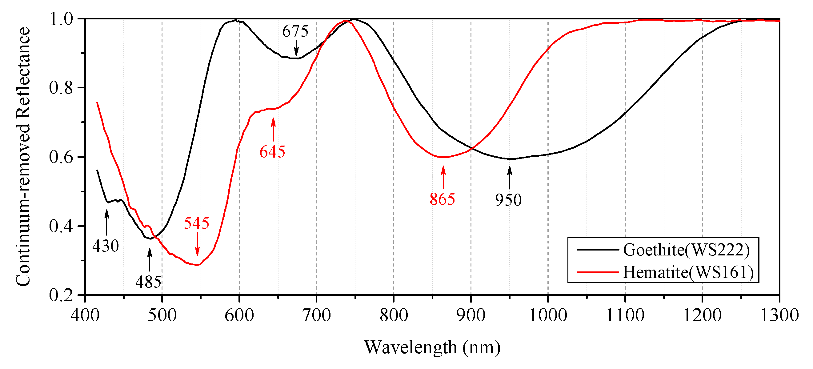
The iron oxides are the most active factor in the visible and near-infrared (VNIR) range because nearly all electric features in this range are produced from various forms of iron [57]. Crystalline iron was responsible for concavities in the 450, 850 and 1100 nm, but amorphous iron only reduced the intensity of reflectance and did not alter the concavities [58]. Goethite and hematite are the most well-known iron oxides and have respective characteristic absorption features (Figure 8). Ben-Dor et al. [25] indicated that the position of the absorption feature of goethite and hematite mixture shifted between the original absorption of the pure mineral absorption and this shift in the Fe absorption features enabled the recognition of hematite and goethite occurrences. In this study, the presence of distinct absorption features near 420, 485–490, 660–670 and 900–910 nm in the spectral curves following continuum-removed spectra indicated the presence of more goethite and little hematite in these soil samples. However, these absorption features of Fe did not present evident changes with soil age.
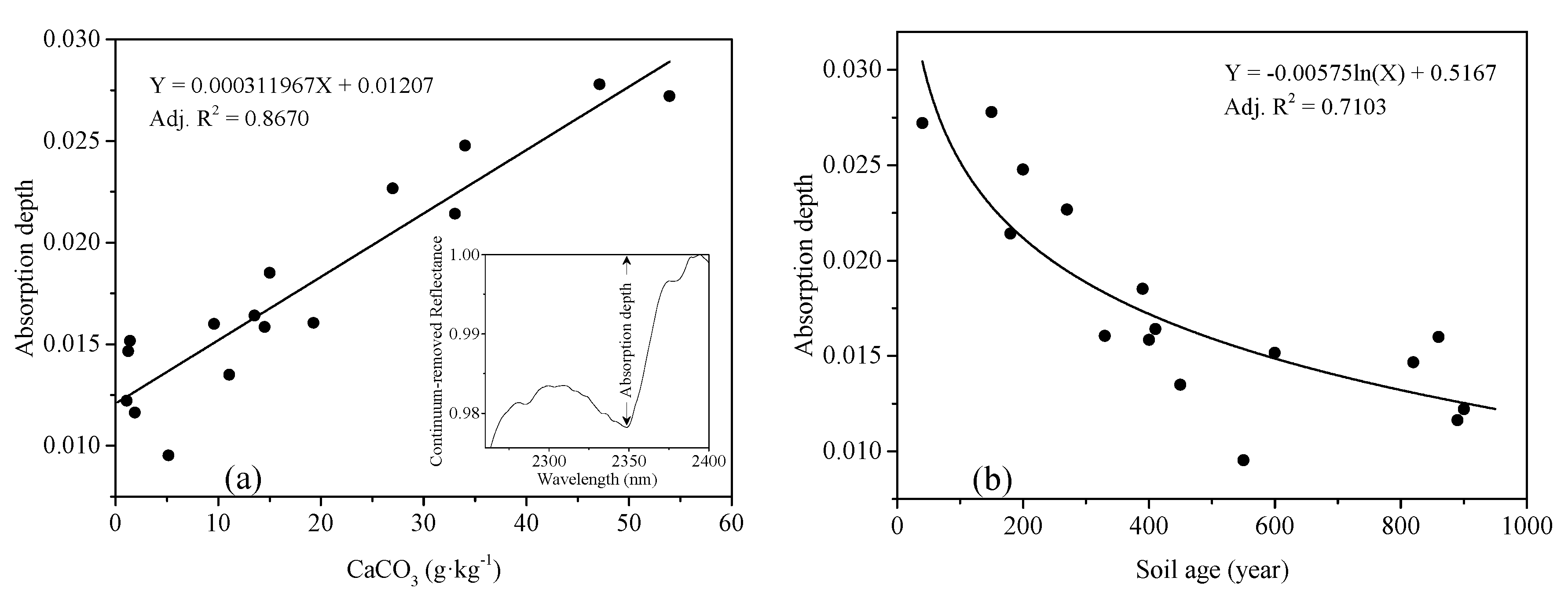
Hunt and Salisbury [59] concluded that five characteristic bands appear near 1900, 2000, 2160, 2350 and 2550 nm for carbonates in the NIR range. The absorption feature of CaCO3 near 2341 nm can be used to estimate carbonate content via continuum-removed reflectance spectroscopy [60,61,62]. In this study, the absorption depth at 2345 nm decreased from younger soil to older soil with a decrease in CaCO3 in every group (Figure 7b,d,f). This absorption depth at 2345 nm was positively correlated with CaCO3, i.e., the absorption depth increased linearly with increasing CaCO3 content (Figure 9a). In addition, the change in the absorption depth at 2345 nm with soil age is distinct and a logarithm function fitted the relationship between the absorption depth and soil age (Adj. R2 = 0.7103) (Figure 9b). Therefore, we can conclude that the spectral feature near 2345 nm can be used to estimate the CaCO3 content and to reveal the soil CaCO3 leaching process in this area.
The obvious absorption features near 1412, 1918, 2210, 2345 and 2445 nm and the two shoulders near 1465 and 2095 nm in these CR curves (Figure 7b,d,f) suggested that the clay mineral in these soil samples is mainly illite. Montmorillonite has absorptions near 1412, 1918, 2210 and the two shoulders, but the absorption depth at 2210 nm is near half of that at 1918 nm (Figure 10). Therefore, montmorillonite is also present in these samples.
3.4. Soil Property Predictions
The PLSR results for the soil properties of the calibration and prediction with smoothed spectra are shown in Table 3. Good and excellent calibrations and prediction ( ≥ 0.80, ≥ 0.80 and RPD ≥ 2.30) were obtained for SOM, CaCO3, and clay. The pH, crystalline Fe and Fed/Fet produced an acceptable result ( ≥ 0.37, ≥ 0.31 and RPD ≥ 1.23).
Complex SOM components complicate the assignment of absorption features to specific functional groups [63,64], although Viscarra Rossel and Behrens [35] concluded that SOC is related to wavelengths that represent absorptions due to organic molecules and proteins. SOM is the most frequently studied soil property via reflectance spectroscopy and the prediction results were superior [20], even at a large scale [65]. In this study, the SOM model provided the best results among six properties (RPD = 3.04).
The CaCO3-leaching process exhibited an inverse trend with SOM accumulation (Figure 5c and Figure 6c), producing a negative correlation between CaCO3 and SOM (Table 2). This correlation and the absorption features of carbonate (2345 nm) may render it possible to predict CaCO3 levels in the soils studied.
The fact that clay is primarily composed of phyllosilicate minerals with special features and the correlation between clay and iron oxides (Table 2) might have contributed to the clay prediction via reflectance spectroscopy [35,63,66]. The pH value, a chemical property, is spectrally featureless, thus its correlation with clay, CaCO3 and SOM (Table 2) was an important prediction mechanism [67]. The diagnostic absorption features can be used to calibrate the content of Fed in soil [68,69,70], which makes it possible to predict Fed.
3.5. Soil Age Calibration Using Spectra From Multiple Depths
In this study area, the absolute soil age is indicative of the development degree of the soil profile. Eight partial least squares regressions were constructed with soil age data as the response variable and spectral data as the predictor variable. The predictor variables were multi-depth soil spectral curves after continuum-removal transformation from the topsoil (one layer) to the entire profile (eight layers), respectively.
Soil chronosequence reflectance spectroscopy can be used to predict soil ages (Table 4). In general, all the models achieved fair or good results (RPD > 1.57). The number of principal components increased with the soil layer number. The calibration results () decreased slightly and increased remarkably with the soil layer number. Otherwise, the prediction results began to decrease after they reached the best result (RPD = 1.85). That is to say that more principal components extracted from more soil layers did not produce better prediction results. The topsoil regression results (0–5 cm) were acceptable because topsoil properties, such as SOM, clay, and CaCO3, changed with soil age (Figure 6a–c). Obtaining the chemical and physical properties of more layers provided more information on pedogenic processes than those of the topsoil (0–5 cm). Therefore, better results should be obtained when additional layer spectral curves are used to calibrate the soil age. Although the two- or three-layer spectra did not produce better calibration and prediction results than topsoil as we supposed, the prediction results for four layers (0–30 cm) were best. The possible reason is that four-layer soil contains more pedogenic information than topsoil and the pseudo multi-depth spectra, joined by four-layer spectra, includes enough information about the difference between soil profiles of different degrees of development.
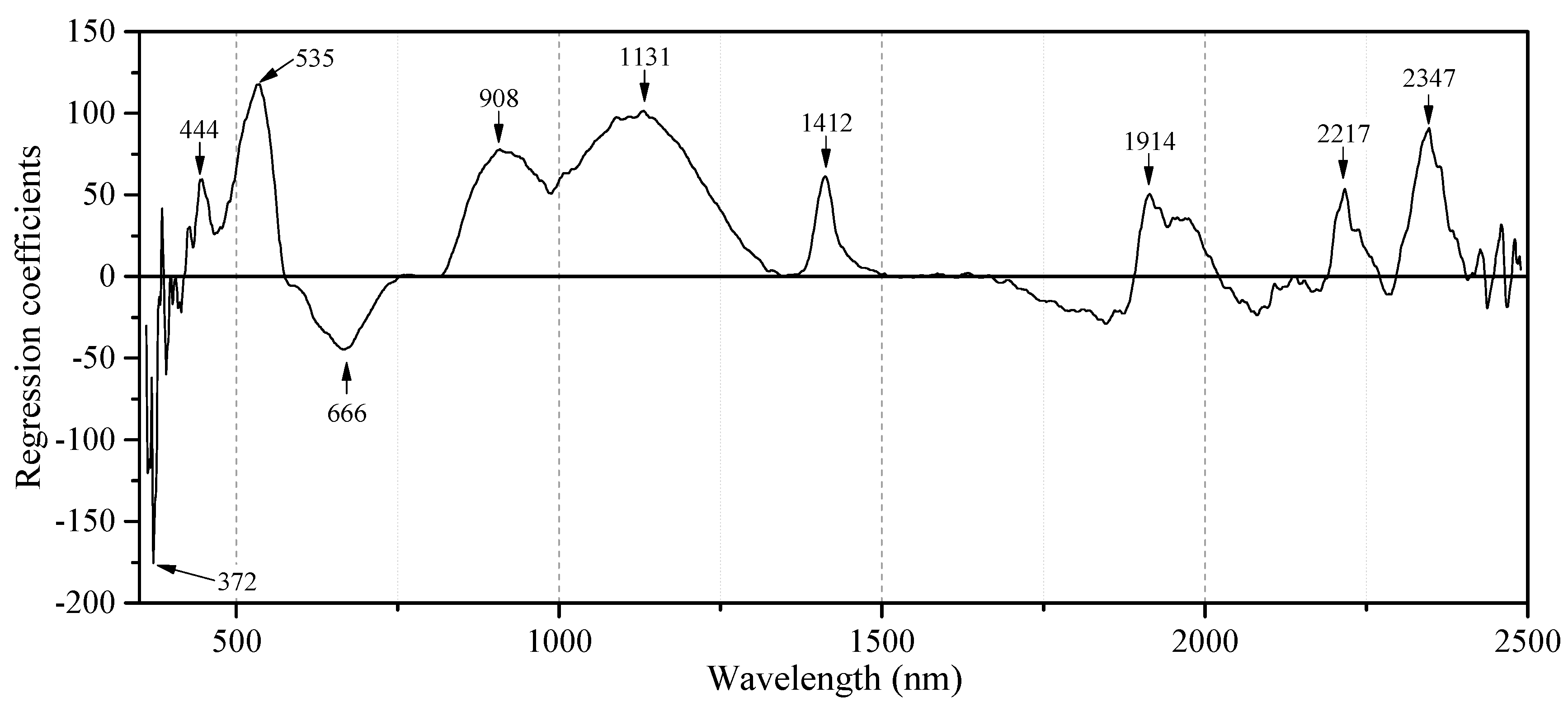
The regression coefficients can show the importance of the specific wavelength. These important wavelengths (Figure 11) included all the absorption features in the continuum-removed spectra in Figure 7. These absorption features are attributed to Fe (372, 444, 535, 666, 908 and 1131 nm), clay minerals (1412, 1914 and 2217 nm) and CaCO3 (2347 nm). This suggested that these soil properties, producing these absorption features, were very important in the calibration and prediction of profile age.
The correlation coefficients were calculated to analyze which soil properties were correlated with the two latent variables in the topsoil model (Table 5). These two latent variables explained 68% and 12% of the spectroscopy information, respectively. The 1st latent variable is positively correlated with SOM and clay and negatively correlated with CaCO3. The correlation coefficients between the second latent variable and clay and CaCO3 were significant. Although it is very difficult to assign the absorption features to SOM, SOM is one of the most important properties in the calibration and prediction of profile age. We can conclude that these three soil properties, SOM, clay and CaCO3, changed with soil age and primarily resulted in the observed changes in the spectra. Thus, the changing soil properties with time act as a bridge and make it possible to analyze soil age or pedogenic processes with spectroscopy.
4. Discussion
4.1. Reflectance Spectroscopy and Soil Genesis
Soil visible and near-infrared (VNIR) diffuse reflectance can provide rich information on soil physical and chemical properties, which implies the possibility of using soil spectroscopy to aid in the analysis of soil genesis. Our results showed that pedogenic processes, such as SOM accumulation and CaCO3 leaching, can be evaluated, and iron oxides and clay minerals can be identified by soil spectroscopy. The application of soil spectroscopy in soil genesis is mainly divided into the following aspects: firstly, the soil weathering degree or weathering indices can be estimated using spectral reflectance [24,71]. Furthermore, Crouvi et al. [72] found that it is possible to map alluvial ages by measuring spectral parameters of three independent chromophores, namely, iron, clay, and carbonates. Secondly, pedogenetic processes, such as organic carbon accumulation, oxide iron variation, and soil rubification process, were identified with soil spectral reflectance [26,28]. Thirdly, soil genetic horizons were distinguished or recognized, and horizon boundaries were defined using soil spectroscopy [73,74,75]. Fajardo et al. [74] indicated that soil spectroscopy offers more information than the traditional description and avoids observer bias when describing a soil core. In addition, soil classes were identified or allocated with surface or profile spectral reflectance [76,77,78,79,80,81]. Since the use of soil spectral reflectance applied to soil science studies has seen exponential growth in the past decades, a new term “spectral pedology” was defined by Demattê and Terra [28].
4.2. Combination of Horizontal Spectroscopy
The study object of soil genesis should be the entire soil profile, not only topsoil or a certain horizon. Therefore, a critical issue when using this new methodology to characterize the entire soil profile is how to combine the spectroscopy of soil horizons for individual profiles [78]. At present, there are four methods to integrate spectral curves for the soil profile. Viscarra Rossel and Webster [73] averaged the spectra for topsoil and subsoil to represent the spectra of a profile. This simple average method may weaken some spectral features of a certain genetic horizon. Vasques et al. [41] constructed a pseudo multi-depth spectrum for profiles by combining the spectra for three depth layers sequentially. This method effectively retains the spectral information for every horizon, but it can be used only when the number of spectral curves in each profile is the same. Thirdly, Ogen et al. [75] used hyper-depth spectral data to classify soils and distinguish soil horizons, where the X-axis presents the wavelength in nm, the y-axis is the depth in cm, and the color scale displays the reflectance value. This method translated the spectral curves in a profile into a spectral surface and retained all the information contained in soil spectroscopy. However, Fajardo et al. [74] found that the depth interval should be ≤2 cm in order to efficiently capture the soil depth changes in a soil core. Therefore, this spectral surface can be used to classify soil classes, but a smaller sampling interval is needed to distinguish the genetic horizon. The last method is to integrate the spectra of a genetic horizon by depth-weighted averaging [78], similar to the method of Viscarra Rossel and Webster [73]. The above methods serve as efficient tools for integrating spectra of legacy soil samples. For the future profile study, Ben-Dor et al. [82] noted that imaging spectroscopy (IS) technology can provide high spectral and spatial resolution data and has the ability to track chemical and physical properties that can serve as tracers to monitor soil genesis and formation.
4.3. Limitation of Research
This work attempted to estimate the profile age in a chronosequence with combined spectral data and obtained a good performance. In this study, the pedogenic properties, such as SOM, clay, and CaCO3, which change with time and are spectrally active, act as the bridge between the profile age or pedogenic processes and spectra. However, this result only suggested the feasibility of this study area and more study in this direction is still required for other chronosequences. It is possible that other properties, such as clay minerals and iron oxides, would be important for spectral analysis and age prediction in a chronosequence of tens of thousands or millions of years.
5. Conclusions
Changing soil properties in a chronosequence that are produced through different weathering levels and pedogenic processes can be reflected through spectral behaviors. These properties serve as a bridge linking soil spectroscopy and weathering levels/pedogenic processes. This study, conducted using a coastal soil chronosequence developed on fairly uniform calcareous marine sediments, demonstrated that profile spectroscopy can detect property changes in a chronosequence and be further used to calibrate soil age.
In this millennium chronosequence, soil pedogenic processes, such as SOM accumulation, CaCO3 leaching and clay migration were detectible. Fed and Fed/Fet did not show remarkable sequential changes with soil age. These three soil properties changing with soil age, SOM, clay and CaCO3, primarily resulted in the observed changes in the spectra. Therefore, these pedogenic processes can be reflected through the reflectance intensity and absorption features of soil spectroscopy. These soil properties, some of which are featureless, can be calibrated through soil reflectance spectroscopy. The pseudo multi-depth spectral curve of a soil profile, a method used to integrate reflectance spectroscopy data for various depths, provided more information on pedogenic processes and produced better soil age calibration and prediction than a spectral curve of topsoil. However, more profiles are needed in the future to further prove this conclusion, and this idea and method can be used in other regions and calibration models according to local soil samples.
Therefore, soil spectroscopy for chronosequence study not only serves as a new technique for pedogenesis research but also represents a new application of spectroscopy techniques. Further studies on how spectroscopy can be applied to chronosequences of other time scales are needed, e.g., a chronosequence of millions of years. The other properties, such as clay minerals and iron oxides, may be important properties for spectral analysis and age prediction in the thousands or millions of years chronosequence.
Author Contributions
Conceptualization, G.Z.; formal analysis, C.J.; investigation, G.S.; writing—original draft preparation, G.Z. and C.J.; writing—review and editing, D.R., X.X. and X.C.; visualization, C.J.; supervision, G.Z.; project administration, G.Z.; funding acquisition, G.Z.
Funding
This research was funded by the National Natural Science Foundation of China (41201215 and 41877004) and the China Scholarship Council (201808320124).
Acknowledgments
We are grateful to Yuguo Zhao and Jingchen Zheng for their assistance during the field sampling work. We thank Changqiao Hong, Junfeng Xiong, Minmin Huang, Yuting Tao, Yongwei Gan, Jiangjie Jia, and Cheng Lv for the sample processing and spectral measurements. We thank all the reviewers for their excellent comments and suggestions to improve the paper.
Conflicts of Interest
The authors declare no conflict of interest.
References
- Jenny, H. Factors of Soil Formation: A System of Quantitative Pedology, 1st ed.; McGraw-Hill: New York, NY, USA, 1941. [Google Scholar]
- Stevens, P.R.; Walker, T.W. The chronosequence concept and soil formation. Q. Rev. Biol. 1970, 45, 333–350. [Google Scholar] [CrossRef]
- Yaalon, D.H. Climate, time and soil development. In Pedogenesis and Soil Taxonomy: I. Concepts and Interactions, 1st ed.; Wilding, L.P., Smeck, N.E., Hall, G.F., Eds.; Elsevier: Amsterdam, The Netherlands, 1983; pp. 223–251. [Google Scholar]
- Jenny, H. The Soil Resource: Origin and Behaviour, 1st ed; Springer: New York, NY, USA, 1980. [Google Scholar]
- Huggett, R.J. Soil chronosequences, soil development, and soil evolution: A critical review. Catena 1998, 32, 155–172. [Google Scholar] [CrossRef]
- Huang, L.M.; Thompson, A.; Zhang, G.L.; Chen, L.M.; Han, G.Z.; Gong, Z.T. The use of chronosequences in studies of paddy soil evolution: A review. Geoderma 2015, 237–238, 199–210. [Google Scholar] [CrossRef]
- Fu, Q.L.; Ding, N.F.; Liu, C.; Lin, Y.C.; Guo, B. Soil development under different cropping systems in a reclaimed coastal soil chronosequence. Geoderma 2014, 230–231, 50–57. [Google Scholar] [CrossRef]
- Vilmundardóttir, O.K.; Gísladóttir, G.; Lal, R. Soil carbon accretion along an age chronosequence formed by the retreat of the Skaftafellsjökull glacier, SE-Iceland. Geomorphology 2015, 228, 124–133. [Google Scholar] [CrossRef]
- Schwertmann, U. The effect of pedogenic environments on iron oxide minerals. In Advances in Soil Science, 1st ed.; Stewart, B.A., Ed.; Springer: New York, NY, USA, 1985; pp. 171–200. [Google Scholar]
- Huang, W.S.; Jien, S.H.; Tsai, H.; Hseu, Z.Y.; Huang, S.T. Soil evolution in a tropical climate: An example from a chronosequence on marine terraces in Taiwan. Catena 2016, 139, 61–72. [Google Scholar] [CrossRef]
- He, Y.; Li, D.C.; Velde, B.; Yang, Y.F.; Huang, C.M.; Gong, Z.T.; Zhang, G.L. Clay minerals in a soil chronosequence derived from basalt on Hainan Island, China and its implication for pedogenesis. Geoderma 2008, 148, 206–212. [Google Scholar] [CrossRef]
- Torrent, J.; Nettleton, W.D. A simple textural index for assessing chemical weathering in soils. Soil Sci. Soc. Am. J. 1979, 43, 373–377. [Google Scholar] [CrossRef]
- Vidic, N.J.; Lobnlk, F. Rates of soil development of the chronosequence in the Ljubljana Basin, Slovenia. Geoderma 1997, 76, 35–64. [Google Scholar] [CrossRef]
- Scarciglia, F.; Pelle, T.; Pulice, I.; Robustelli, G. A comparison of quaternary soil chronosequences from the ionian and tyrrhenian coasts of calabria, southern italy: Rates of soil development and geomorphic dynamics. Quatern. Int. 2015, 376, 146–162. [Google Scholar] [CrossRef]
- Merritts, D.J.; Chadwick, O.A.; Hendricks, D.M. Rates and processes of soil evolution on uplifted marine terraces, northern California. Geoderma 1991, 51, 241–275. [Google Scholar] [CrossRef]
- Schaetzl, R.J.; Anderson, S. Soils: Genesis and Geomorphology, 1st ed.; Cambridge University Press: New York, NY, USA, 2005. [Google Scholar]
- Viscarra Rossel, R.A.; Walvoort, D.J.J.; McBratney, A.B.; Janik, L.J.; Skjemstad, J.O. Visible, near infrared, mid infrared or combined diffuse reflectance spectroscopy for simultaneous assessment of various soil properties. Geoderma 2006, 131, 59–75. [Google Scholar] [CrossRef]
- Bowers, S.A.; Hanks, R.J. Reflectance of radiant energy from soils. Soil Sci. 1965, 100, 130–138. [Google Scholar] [CrossRef]
- Condit, H.R. The spectral reflectance of American soils. Photogramm. Eng. 1970, 36, 955–966. [Google Scholar]
- Stenberg, B.; Viscarra Rossel, R.A.; Mouazen, A.M.; Wetterlind, J.; Donald, L.S. Visible and near infrared spectroscopy in soil science. Adv. Agron. 2010, 107, 163–215. [Google Scholar] [CrossRef]
- Viscarra Rossel, R.A.; Lobsey, C.R.; Sharman, C.; Flick, P.; McLachlan, G. Novel soil profile sensing to monitor organic C stocks and condition. Environ. Sci. Technol. 2017, 51, 5630–5641. [Google Scholar] [CrossRef]
- Demattê, J.A.M.; Fongaro, C.T.; Rizzo, R.; Safanelli, J.L. Geospatial Soil Sensing System (GEOS3): A powerful data mining procedure to retrieve soil spectral reflectance from satellite images. Remote Sens. Environ. 2018, 212, 161–175. [Google Scholar] [CrossRef]
- Peng, J.; Biswas, A.; Jiang, Q.S.; Zhao, R.Y.; Hu, J.; Hu, B.F.; Shi, Z. Estimating soil salinity from remote sensing and terrain data in southern Xinjiang Province, China. Geoderma 2019, 337, 1309–1319. [Google Scholar] [CrossRef]
- Demattê, J.A.M.; Garcia, G.J. Alteration of soil properties through a weathering sequence as evaluated by spectral reflectance. Soil Sci. Soc. Am. J. 1999, 63, 327–342. [Google Scholar] [CrossRef]
- Ben-Dor, E.; Levin, N.; Singer, A.; Karnieli, A.; Braun, O.; Kidron, G.J. Quantitative mapping of the soil rubification process on sand dunes using an airborne hyperspectral sensor. Geoderma 2006, 131, 1–21. [Google Scholar] [CrossRef]
- Demattê, J.A.M.; Horák-Terra, I.; Beirigo, R.M.; Terra, F.S.; Marques, K.P.P.; Fongaro, C.T.; Silva, A.C.; Vidal-Torrado, P. Genesis and properties of wetland soils by VIS-NIR-SWIR as a technique for environmental monitoring. J. Environ. Manage. 2017, 197, 50–62. [Google Scholar] [CrossRef]
- Terra, F.S.; Demattê, J.A.M.; Viscarra Rossel, R.A. Proximal spectral sensing in pedological assessments: Vis–NIR spectra for soil classification based on weathering and pedogenesis. Geoderma 2018, 318, 123–136. [Google Scholar] [CrossRef]
- Demattê, J.A.M.; Terra, F.D.S. Spectral pedology: A new perspective on evaluation of soils along pedogenetic alterations. Geoderma 2014, 217–218, 190–200. [Google Scholar] [CrossRef]
- Zheng, G.H.; Jiao, C.X.; Zhou, S.L.; Shang, G. Analysis of soil chronosequence studies using reflectance spectroscopy. Int. J. Remote Sens. 2016, 37, 1881–1901. [Google Scholar] [CrossRef]
- Awiti, A.O.; Walsh, M.G.; Shepherd, W.K.; Kinyamario, J. Soil condition classification using infrared spectroscopy: A proposition for assessment of soil condition along a tropical forest-cropland chronosequence. Geoderma 2008, 143, 73–84. [Google Scholar] [CrossRef]
- Chen, L.M.; Zhang, G.L.; Effland, W.R. Soil characteristic response times and pedogenic thresholds during the 1000-year evolution of a paddy soil chronosequence. Soil Sci. Soc. Am. J. 2011, 75, 1807–1820. [Google Scholar] [CrossRef]
- Cui, J.; Liu, C.; Li, Z.L.; Wang, L.; Chen, X.F.; Ye, Z.Z.; Fang, C.M. Long-term changes in topsoil chemical properties under centuries of cultivation after reclamation of coastal wetlands in the Yangtze Estuary, China. Soil Till Res. 2012, 123, 50–60. [Google Scholar] [CrossRef]
- Zhang, R.S. Land-forming history of the Huanghe River delta and coastal plain of north Jiangsu. Acta Geogr. Sin. 1984, 39, 173–184. [Google Scholar]
- Lu, R.K. Chemical Analysis of Agricultural Soil, 1st ed.; China Agricultural Science and Technology Press: Beijing, China, 1999. [Google Scholar]
- Viscarra Rossel, R.A.; Behrens, T. Using data mining to model and interpret soil diffuse reflectance spectra. Geoderma 2010, 158, 46–54. [Google Scholar] [CrossRef]
- Wold, S.; Martens, H.; Wold, H. The multivariate calibration method in chemistry solved by the PLS method. In Lecture Notes in Mathematics; Kågström, B., Ruhe, A., Eds.; Springer: Heidelberg, German, 1983; pp. 286–293. [Google Scholar] [CrossRef]
- Dangal, S.R.S.; Sanderman, J.; Wills, S.; Ramirez-Lopez, L. Accurate and precise prediction of soil properties from a large mid-infrared spectral library. Soil Syst. 2019, 3, 11. [Google Scholar] [CrossRef]
- Clark, R.N.; Roush, T.L. Reflectance spectroscopy: Quantitative analysis techniques for remote sensing applications. J. Geophys. Res. 1984, 89, 6329–6340. [Google Scholar] [CrossRef]
- Viscarra Rossel, R.A.; Cattle, S.R.; Ortega, S.R.; Fouad, Y. In situ measurements of soil colour, mineral composition and clay content by vis-NIR spectroscopy. Geoderma 2009, 150, 253–266. [Google Scholar] [CrossRef]
- Savitzky, A.; Golay, M.J.E. Smoothing and differentiation of data by simplified least squares procedures. Anal. Chem. 1964, 36, 1627–1639. [Google Scholar] [CrossRef]
- Vasques, G.M.; Demattê, J.A.M.; Viscarra Rossel, R.A.; Ramírez-López, L.; Terra, F.S. Soil classification using visible/near-infrared diffuse reflectance spectra from multiple depths. Geoderma 2014, 223–225, 73–78. [Google Scholar] [CrossRef]
- Minasny, B.; Stockmann, U.; Hartemink, A.E.; McBratney, A.B. Measuring and modelling soil depth functions. In Digital Soil Morphometrics; Hartemink, E.A., Minasny, B., Eds.; Springer: Cham, Switzerland, 2016; pp. 225–240. [Google Scholar] [CrossRef]
- Brauer, T.; Grootes, P.M.; Nadeau, M.J.; Andersen, N. Downward carbon transport in a 2000-year rice paddy soil chronosequence traced by radiocarbon measurements. Nucl. Inst. Methods Phys. Res. B 2012, 294, 584–587. [Google Scholar] [CrossRef]
- VandenBygaart, A.J.; Protz, R. Soil genesis on a chronosequence, Pinery Provincial Park, Ontario. Can. J. Soil Sci. 1995, 75, 63–72. [Google Scholar] [CrossRef] [Green Version]
- Zhao, Y.G.; Liu, X.F.; Wang, Z.L.; Zhao, S.W. Soil organic carbon fractions and sequestration across a 150-yr secondary forest chronosequence on the Loess Plateau, China. Catena 2015, 133, 303–308. [Google Scholar] [CrossRef]
- Bockheim, J.G.; Marshall, J.G.; Kelsey, H.M. Soil-forming processes and rates on uplifted marine terraces in southwestern Oregon, USA. Geoderma 1996, 73, 39–62. [Google Scholar] [CrossRef]
- Burkins, D.L.; Blum, J.D.; Brown, K.; Reynolds, R.C.; Erel, Y. Chemistry and mineralogy of a granitic, glacial soil chronosequence, Sierra Nevada Mountains, California. Chem. Geol. 1999, 162, 1–14. [Google Scholar] [CrossRef]
- He, Y.R.; Huang, C.M.; Xu, X.M.; Wang, Y.Q.; He, X.B. Micromorphological features of Paleo-Stagnic-Anthrosols at archaeological site of Sanxingdui, China. J. Mountain Sci. 2008, 5, 358–366. [Google Scholar] [CrossRef]
- Bockheim, J.G. Solution and use of chronofunctions in studying soil development. Geoderma 1980, 24, 71–85. [Google Scholar] [CrossRef]
- Wissing, L.; Kolbl, A.; Vogelsang, V.; Fu, J.R.; Cao, Z.H.; Kogel-Knabner, I. Organic carbon accumulation in a 2000-year chronosequence of paddy soil evolution. Catena 2011, 87, 376–385. [Google Scholar] [CrossRef]
- Badía, D.; Martí, C.; Casanova, J.; Gillot, T.; Cuchí, J.A.; Palacio, J.; Andrés, R. A Quaternary soil chronosequence study on the terraces of the Alcanadre River (semiarid Ebro Basin, NE Spain). Geoderma 2015, 241–242, 158–167. [Google Scholar] [CrossRef]
- Muhs, D.R. Intrinsic thresholds in soil systems. Phys. Geogr. 1984, 5, 99–110. [Google Scholar] [CrossRef]
- Torrent, J.; Schwertmann, U.; Schulze, D.G. Iron oxide mineralogy of some soils of two river terrace sequences in Spain. Geoderma 1980, 23, 191–208. [Google Scholar] [CrossRef]
- Stoner, E.R.; Baumgardner, M.F. Characteristic variations in reflectance of surface soils. Soil Sci. Soc. Am. J. 1981, 45, 1161–1165. [Google Scholar] [CrossRef]
- Ben-Dor, E. Quantitative remote sensing of soil properties. Adv. Agron. 2002, 75, 173–243. [Google Scholar] [CrossRef]
- Demattê, J.A.M.; Campos, R.C.; Alves, M.C.; Fiorio, P.R.; Nanni, M.R. Visible-NIR reflectance: A new approach on soil evaluation. Geoderma 2004, 121, 95–112. [Google Scholar] [CrossRef]
- Hunt, G.R.; Salisbury, J.W. Visible and near-infrared spectra of minerals and rocks: I Silicate minerals. Mod. Geol. 1970, 1, 283–300. [Google Scholar]
- Demattê, J.A.M.; Nanni, M.R.; Formaggio, A.R.; Epiphanio, J.C.N. Spectral reflectance for the mineralogical evaluation of Brazilian low clay activity soils. Int. J. Remote Sens. 2007, 28, 4537–4559. [Google Scholar] [CrossRef]
- Hunt, G.R.; Salisbury, J.W. Visible and near infrared spectra of minerals and rocks: II Carbonates. Mod. Geol. 1971, 2, 23–30. [Google Scholar]
- Lagacherie, P.; Baret, F.; Feret, J.; Netto, J.M.; Robbez-Masson, J.M. Estimation of soil clay and calcium carbonate using laboratory, field and airborne hyperspectral measurements. Remote Sens. Environ. 2008, 112, 825–835. [Google Scholar] [CrossRef]
- Gomez, C.; Lagacherie, P.; Coulouma, G. Continuum removal versus PLSR method for clay and calcium carbonate content estimation from laboratory and airborne hyperspectral measurements. Geoderma 2008, 148, 141–148. [Google Scholar] [CrossRef]
- Hong, C.Q.; Zheng, G.H.; Chen, C.C. Estimation of CaCO3 content in coastal soil of North Jiangsu with reflectance spectroscopy. Acta Pedol. Sin. 2016, 53, 1120–1129. [Google Scholar] [CrossRef]
- Ben-Dor, E.; Banin, A. Near-infrared analysis as a rapid method to simultaneously evaluate several soil properties. Soil Sci. Soc. Am. J. 1995, 59, 364–372. [Google Scholar] [CrossRef]
- Chang, C.W.; Laird, D.A. Near-infrared reflectance spectroscopic analysis of soil C and N. Soil Sci. 2002, 167, 110–116. [Google Scholar] [CrossRef]
- Stevens, A.; Nocita, M.; Tóth, G.; Montanarella, L.; Wesemael, B. Prediction of soil organic carbon at the European scale by visible and near infrared reflectance spectroscopy. PloS ONE 2013, 8, 1–13. [Google Scholar] [CrossRef]
- Jaconi, A.; Vos, C.; Don, A. Near infrared spectroscopy as an easy and precise method to estimate soil texture. Geoderma 2019, 337, 906–913. [Google Scholar] [CrossRef]
- Ben-Dor, E.; Banin, A. Visible and near-infrared (0.4-1.1 um) analysis of arid and semiarid soils. Remote Sens. Environ. 1994, 48, 261–274. [Google Scholar] [CrossRef]
- Bartholomeus, H.; Epema, G.; Schaepman, M. Determining iron content in Mediterranean soils in partly vegetated areas, using spectral reflectance and imaging spectroscopy. Int. J. Appl. Earth. Obs. 2007, 9, 194–203. [Google Scholar] [CrossRef] [Green Version]
- Ben-Dor, E.; Heller, D.; Chudnovsky, A. A novel method of classifying soil profiles in the field using optical means. Soil Sci. Soc. Am. J. 2008, 72, 1113–1123. [Google Scholar] [CrossRef]
- Richter, N.; Jarmer, T.; Chabrillat, S.; Oyonarte, C.; Hostert, P.; Kaufmann, H. Free iron oxide determination in mediterranean soils using diffuse reflectance spectroscopy. Soil Sci. Soc. Am. J. 2009, 73, 72–81. [Google Scholar] [CrossRef]
- Mohanty, B.; Gupta, A.; Das, B.S. Estimation of weathering indices using spectral reflectance over visible to mid-infrared region. Geoderma 2016, 266, 111–119. [Google Scholar] [CrossRef]
- Crouvi, O.; Ben-Dor, E.; Beyth, M.; Avigad, D.; Amit, R. Quantitative mapping of arid alluvial fan surfaces using field spectrometer and hyperspectral remote sensing. Remote Sens. Environ. 2006, 104, 103–117. [Google Scholar] [CrossRef]
- Viscarra Rossel, R.A.; Webster, R. Discrimination of Australian soil horizons and classes from their visible–near infrared spectra. Eur. J. Soil Sci. 2011, 62, 637–647. [Google Scholar] [CrossRef]
- Fajardo, M.; McBratney, A.; Whelan, B. Fuzzy clustering of Vis-NIR spectra for the objective recognition of soil morphological horizons in soil profiles. Geoderma 2016, 263, 244–253. [Google Scholar] [CrossRef]
- Ogen, Y.; Goldshleger, N.; Ben-Dor, E. 3D spectral analysis in the VNIR-SWIR spectral region as a tool for soil classification. Geoderma 2017, 302, 100–110. [Google Scholar] [CrossRef]
- Zhang, X.K.; Liu, H.J.; Zhang, X.L.; Yu, S.N.; Dou, X.; Xie, Y.H.; Wang, N. Allocate soil individuals to soil classes with topsoil spectral characteristics and decision trees. Geoderma 2018, 320, 12–22. [Google Scholar] [CrossRef]
- Teng, H.; Viscarra Rossel, R.A.; Shi, Z.; Behrens, T. Updating a national soil classification with spectroscopic predictions and digital soil mapping. Catena 2018, 164, 125–134. [Google Scholar] [CrossRef]
- Xie, X.L.; Li, A.B. Identification of soil profile classes using depth-weighted visible–near-infrared spectral reflectance. Geoderma 2018, 325, 90–101. [Google Scholar] [CrossRef]
- Wang, X.; Zhang, X.K.; Li, H.X.; Zhang, X.L.; Liu, H.J.; Dou, X.; Yu, Z.Y. The minimum level for soil allocation using topsoil reflectance spectra: Genus or species? Catena 2019, 174, 36–47. [Google Scholar] [CrossRef]
- Zeng, R.; Rossiter, D.G.; Yang, F.; Li, D.C.; Zhao, Y.G.; Zhang, G.L. How accurately can soil classes be allocated based on spectrally predicted physio-chemical properties? Geoderma 2017, 303, 78–84. [Google Scholar] [CrossRef]
- Zeng, R.; Rossiter, D.G.; Zhang, G.L. How compatible are numerical classifications based on whole-profile vis–NIR spectra and the Chinese Soil Taxonomy? Eur. J. Soil Sci. 2019, 70, 54–65. [Google Scholar] [CrossRef]
- Ben-Dor, E.; Chabrillat, S.; Demattê, J.A.M.; Taylor, G.R.; Hill, J.; Whiting, M.L.; Sommer, S. Using imaging spectroscopy to study soil properties. Remote Sens. Environ. 2009, 113, 38–55. [Google Scholar] [CrossRef]
Figure 1.
Coastline changes in Jiangsu Province, China [33].
Figure 1.
Coastline changes in Jiangsu Province, China [33].

Figure 2.
Locations of soil profiles and sampling depth in a profile: (a) sixteen sampling sites, which, generally, ran perpendicular to the coastlines; The soil ages were estimated based on the historical coastlines [33]; (b) eight samples were collected from every profiles according to the following intervals: 0–5, 5–10, 10–20, 20–30, 30–40, 40–60, 60–80 and 80–100 cm.

Figure 3.
Optical setup of the spectrometer.

Figure 4.
Pseudo multi-depth curves of smoothed and continuum-removed spectra for partial profiles. The pseudo multi-depth curve was created by joining the spectra from the eight depth intervals of a profile in sequence, which represents the spectra of the whole profile from topsoil to bottom soil.
Figure 4.
Pseudo multi-depth curves of smoothed and continuum-removed spectra for partial profiles. The pseudo multi-depth curve was created by joining the spectra from the eight depth intervals of a profile in sequence, which represents the spectra of the whole profile from topsoil to bottom soil.

Figure 5.
Depth distribution of soil properties depending on the age of soil profiles: (a) soil organic matter (SOM); (b) clay; (c) CaCO3; (d) pH; (e) Fed; (f) Fed/Fet.
Figure 5.
Depth distribution of soil properties depending on the age of soil profiles: (a) soil organic matter (SOM); (b) clay; (c) CaCO3; (d) pH; (e) Fed; (f) Fed/Fet.

Figure 6.
Changes in six soil properties with time in topsoil (0–5 cm) samples: (a) SOM; (b) clay; (c) CaCO3; (d) pH; (e) Fed; (f) Fed/Fet.
Figure 6.
Changes in six soil properties with time in topsoil (0–5 cm) samples: (a) SOM; (b) clay; (c) CaCO3; (d) pH; (e) Fed; (f) Fed/Fet.

Figure 7.
Original and continuum-removed spectra of topsoil samples (0–5 cm): (a), (c), (e): original spectra of topsoil samples for north line, middle line and south line, respectively; (b), (d), (f): continuum-removed spectra of topsoil samples for north line, middle line and south line, respectively. The overall changes in the reflectance intensity of original spectra primarily showed SOM accumulation with age. The changes in the absorption depth at 2341 nm revealed the CaCO3 leaching process with age. The absorption features around 420, 485, 670 and 900 nm in continuum-removed spectra showed the difference in goethite content.


Figure 8.
Continuum-removed spectra of hematite and goethite (the United States Geological Survey (USGS) mineral spectral library). Absorption features around 430, 485, 675, and 950 nm by Goethite and Absorption features around 545, 645, and 865 nm by Hematite.
Figure 8.
Continuum-removed spectra of hematite and goethite (the United States Geological Survey (USGS) mineral spectral library). Absorption features around 430, 485, 675, and 950 nm by Goethite and Absorption features around 545, 645, and 865 nm by Hematite.

Figure 9.
Changes in the absorption depth at 2345 nm with CaCO3 and time. The absorption depth at 2345 nm increases linearly with CaCO3 content (a) and decreases logarithmically with soil age (b).
Figure 9.
Changes in the absorption depth at 2345 nm with CaCO3 and time. The absorption depth at 2345 nm increases linearly with CaCO3 content (a) and decreases logarithmically with soil age (b).

Figure 10.
Continuum-removed spectra of illite and montmorillonite (USGS Mineral spectral library). These two clay minerals have absorptions near 1410, 1918, 2210 and two absorption shoulders near 1465 and 2095 nm.
Figure 10.
Continuum-removed spectra of illite and montmorillonite (USGS Mineral spectral library). These two clay minerals have absorptions near 1410, 1918, 2210 and two absorption shoulders near 1465 and 2095 nm.

Figure 11.
Regression coefficients of topsoil model.


Table 1.
Basic statistics for six soil properties.
| Soil Property | Min | Max | Mean | SD | CV (%) | Skew | Kurt |
|---|---|---|---|---|---|---|---|
| SOM | 1.4 | 33.4 | 7.1 | 6.2 | 86.9 | 1.5 | 2.5 |
| Clay | 1.9 | 18.3 | 7.7 | 4.0 | 51.3 | 0.7 | −0.3 |
| CaCO3 | 0.9 | 63.8 | 30.8 | 16.8 | 54.4 | 0.0 | −1.0 |
| pH | 6.4 | 9.2 | 8.5 | 0.4 | 5.1 | −1.7 | 5.3 |
| Fed | 1.8 | 6.6 | 3.3 | 0.7 | 20.5 | 0.9 | 3.7 |
| Fed/Fet | 7.8 | 26.8 | 15.0 | 3.3 | 21.7 | 0.8 | 2.0 |
Note: Min: minimum; Max: maximum; SD: standard deviation; CV: coefficient of variation; Skew: skewness; Kurt: kurtosis; soil organic matter (SOM): g kg−1; Clay: %; CaCO3: g kg−1; Fed: g kg−1; Fed/Fet: %; Hereinafter inclusive.
Table 2.
Correlation coefficients of six soil properties.
| SOM | Clay | CaCO3 | pH | Fed | Fed/Fet | |
|---|---|---|---|---|---|---|
| SOM | 1.00 | 0.75 ** | −0.64 ** | −0.48 ** | −0.08 | −0.03 |
| Clay | 1.00 | −0.76 ** | −0.41 ** | 0.20 * | 0.21 * | |
| CaCO3 | 1.00 | 0.39 ** | −0.28 ** | −0.33 ** | ||
| pH | 1.00 | 0.09 | 0.10 | |||
| Fed | 1.00 | 0.89 ** | ||||
| Fed/Fet | 1.00 |
Note: ** Significant correlation at the 0.01 level; * Significant correlation at the 0.05 level.
Table 3.
Calibration and prediction of the soil properties.
| Soil Property | LVs Number | Calibration (n = 102) | Cross Validation | Prediction (n = 26) | ||||
|---|---|---|---|---|---|---|---|---|
| RMSEC | RMSECV | RMSEP | RPD | |||||
| SOM | 9 | 1.76 | 0.92 | 2.22 | 0.88 | 1.98 | 0.89 | 3.04 |
| Clay | 9 | 1.35 | 0.89 | 1.74 | 0.82 | 1.62 | 0.81 | 2.33 |
| CaCO3 | 10 | 4.40 | 0.93 | 5.40 | 0.90 | 7.13 | 0.83 | 2.42 |
| pH | 3 | 0.31 | 0.38 | 0.34 | 0.31 | 0.42 | 0.37 | 1.28 |
| Fed | 3 | 0.49 | 0.48 | 0.52 | 0.43 | 0.52 | 0.34 | 1.26 |
| Fed/Fet | 3 | 2.61 | 0.37 | 2.75 | 0.31 | 2.56 | 0.31 | 1.23 |
Note: LVs is latent variables, RMSEC is root mean square error for calibration, RMSECV is root mean square error for cross validation, RMSEP is root mean square error for prediction, is coefficient of determination for calibration, is coefficient of determination for cross validation, is coefficient of determination for prediction, and RPD is residual prediction deviation. Hereinafter inclusive.
Table 4.
Calibration and predication of the profile age using multi-depth spectroscopy.
| Layer Number | Depth | LVs Number | Calibration (n = 10) | Cross Validation | Prediction (n = 6) | ||||
|---|---|---|---|---|---|---|---|---|---|
| RMSEC | RMSECV | RMSEP | RPD | ||||||
| 1 | 0–5 cm | 2 | 131.11 | 0.80 | 188.88 | 0.66 | 138.72 | 0.62 | 1.79 |
| 2 | 0–10 cm | 2 | 137.59 | 0.77 | 198.75 | 0.62 | 157.58 | 0.51 | 1.57 |
| 3 | 0–20 cm | 2 | 141.37 | 0.76 | 206.70 | 0.59 | 155.19 | 0.53 | 1.60 |
| 4 | 0–30 cm | 2 | 133.98 | 0.79 | 201.96 | 0.61 | 133.63 | 0.65 | 1.85 |
| 5 | 0–40 cm | 3 | 99.76 | 0.88 | 167.47 | 0.73 | 140.78 | 0.61 | 1.76 |
| 6 | 0–60 cm | 4 | 80.94 | 0.92 | 177.19 | 0.70 | 145.15 | 0.59 | 1.71 |
| 7 | 0–80 cm | 4 | 78.10 | 0.93 | 187.05 | 0.66 | 148.85 | 0.57 | 1.66 |
| 8 | 0–100 cm | 4 | 72.38 | 0.94 | 201.58 | 0.61 | 154.29 | 0.53 | 1.61 |
Note: Conventions are shown in Table 3.
Table 5.
Correlation coefficients of latent variables and soil properties.
| SOM | Clay | CaCO3 | pH | Fed | Fed/Fet | |
|---|---|---|---|---|---|---|
| LV-1 (68%) | 0.78 ** | 0.52 * | −0.62 * | −0.41 | −0.14 | 0.33 |
| LV-2 (12%) | 0.46 | 0.66 ** | −0.71 ** | −0.37 | 0.39 | 0.35 |
Note: ** significant at the 0.01 level (two-tailed); * significant at the 0.05 level (two-tailed); LV-1: the first latent variable; LV-2: the second latent variable.
© 2019 by the authors. Licensee MDPI, Basel, Switzerland. This article is an open access article distributed under the terms and conditions of the Creative Commons Attribution (CC BY) license (http://creativecommons.org/licenses/by/4.0/).
Share and Cite
MDPI and ACS Style
Zheng, G.; Ryu, D.; Jiao, C.; Xie, X.; Cui, X.; Shang, G. Visible and Near-Infrared Reflectance Spectroscopy Analysis of a Coastal Soil Chronosequence. Remote Sens. 2019, 11, 2336. https://doi.org/10.3390/rs11202336
AMA Style
Zheng G, Ryu D, Jiao C, Xie X, Cui X, Shang G. Visible and Near-Infrared Reflectance Spectroscopy Analysis of a Coastal Soil Chronosequence. Remote Sensing. 2019; 11(20):2336. https://doi.org/10.3390/rs11202336
Chicago/Turabian StyleZheng, Guanghui, Dongryeol Ryu, Caixia Jiao, Xianli Xie, Xuefeng Cui, and Gang Shang. 2019. "Visible and Near-Infrared Reflectance Spectroscopy Analysis of a Coastal Soil Chronosequence" Remote Sensing 11, no. 20: 2336. https://doi.org/10.3390/rs11202336
Note that from the first issue of 2016, this journal uses article numbers instead of page numbers. See further details here.