A GIS-Based Water Balance Approach Using a LiDAR-Derived DEM Captures Fine-Scale Vegetation Patterns

Department of Geography, Ohio University, Athens, OH 45701, USA
Remote Sens. 2019, 11(20), 2385; https://doi.org/10.3390/rs11202385
Submission received: 22 July 2019
/
Revised: 13 October 2019
/
Accepted: 13 October 2019
/
Published: 15 October 2019
(This article belongs to the Special Issue Applications of RS and GIS Integration in Natural Resources and Environmental Science)
Abstract
:Topography exerts strong control on microclimate, resulting in distinctive vegetation patterns in areas of moderate to high relief. Using the Thornthwaite approach to account for hydrologic cycle components, a GIS-based Water Balance Toolset is presented as a means to address fine-scale species–site relationships. For each pixel within a study area, the toolset assesses inter-annual variations in moisture demand (governed by temperature and radiation) and availability (precipitation, soil storage). These in turn enable computation of climatic water deficit, the amount by which available moisture fails to meet demand. Summer deficit computed by the model correlates highly with the Standardized Precipitation–Evapotranspiration Index (SPEI) for drought at several sites across the eastern U.S. Yet the strength of the approach is its ability to model fine-scale patterns. For a 25-ha study site in central Indiana, individual tree locations were linked to summer deficit under different historical conditions: using average monthly climatic variables for 1998–2017, and for the drought year of 2012. In addition, future baseline and drought-year projections were modeled based on downscaled GCM data for 2071–2100. Although small deficits are observed under average conditions (historical or future), strong patterns linked to topography emerge during drought years. The modeled moisture patterns capture vegetation distributions described for the region, with beech and maple preferentially occurring in low-deficit settings, and oak and hickory dominating more xeric positions. End-of-century projections suggest severe deficit, which should favor oak and hickory over more mesic species. Pockets of smaller deficit persist on the landscape, but only when a fine-resolution Light Detection and Ranging (LiDAR)-derived Digital Elevation Model (DEM) is used; a coarse-resolution DEM masks fine-scale variability and compresses the range of observed values. Identification of mesic habitat microrefugia has important implications for retreating species under altered climate. Using readily available data to evaluate fine-scale patterns of moisture demand and availability, the Water Balance Toolset provides a useful approach to explore species–environment linkages.
1. Introduction
Variation in available energy and moisture generate pattern in the abundance, growth, and mortality of plant species, and these patterns manifest across all spatial scales [1]. For example, in North America, deciduous forest occurs in locations with a lengthy growing season defined by temperature, and abundant precipitation that meets the seasonal timing of moisture demand throughout the year [2]. At finer spatial scales, other factors may assume increasing importance, but available moisture and energy continue to influence the distribution of plant species. In upland forested landscapes, topography can exert significant control over temperature and moisture conditions, through its influence on drainage and radiation load. As a result, distinctive vegetation patterns often emerge in areas of moderate to high relief. Slopes with southerly aspects experience higher moisture demand in the northern hemisphere midlatitudes, since they receive more direct insolation. Despite occupying a range of habitats within the eastern deciduous forest, species such as white oak, black oak, and pignut hickory often occur in higher abundance on south-facing aspects, whereas “mesophytes” (species associated with equable moisture conditions) such as beech and sugar maple, are more frequent on north-facing aspects [3,4,5,6,7]. Since these topographic patterns in vegetation are driven by microclimatic variation, an understanding of their potential response to altered climate is of especial interest. At a regional scale, altered patterns of tree species dominance are anticipated with climate change within the next century [8]; less focus has been given to potential fine-scale shifts in species distributions. In southeastern Ohio, shifts in topographic site affinities for individual species have been observed over the past two centuries, with climate change a possible contributing factor [9].
A number of drought indices have been developed that incorporate temperature and precipitation data, and can be used to assess climate change scenarios and the resulting vegetation response. For example, the Palmer Drought Severity Index (PDSI) [10] and the Standardized Precipitation–Evapotranspiration Index (SPEI) [11] both directly assess moisture demand and availability of a place. However, these indices do not produce a continuous surface of moisture relationships, and therefore do not capture topographic variation. With the development of Geographic Information Systems and the availability of Digital Elevation Models (DEMs), a number of topography-based indices have been developed that enable an assessment of moisture patterns across a landscape; two notable examples are the Topographic Wetness Index (TWI) (or Topographic Convergence Index, TCI) [12] and the Integrated Moisture Index (IMI) [13]. These indices focus on drainage to characterize moisture patterns (e.g., TWI: local slope and contributing upslope area, IMI: flow accumulation, curvature); the IMI also incorporates radiation (via “hillshade”) and optionally, soil water-holding capacity. The IMI is scaled 0–100 (xeric–hydric), while the TWI is a relative index, with larger numbers indicating pixels contributing more runoff. Both indices have been linked to spatial variation in ecological attributes e.g., [14,15]. However, both moisture indices are static, in that they do not incorporate precipitation. This limits their applicability to link changes in moisture conditions to ecological attributes over time (e.g., growth rates, mortality), or to explore altered moisture patterns under climate change scenarios.
In contrast, a topographically based water-balance approach that incorporates moisture demand and availability can explicitly account for moisture patterns both spatially and temporally. In a water balance approach, moisture demand is typically defined for a uniform vegetated surface that experiences no lack of water [16]. This moisture demand, or potential evapotranspiration, is expressed as an amount of water, and is especially dependent on temperature and radiation. Depending on the amount of precipitation and soil storage, water may be limiting at the site, and actual evapotranspiration may be less than potential evapotranspiration. The climatic water deficit is the difference between potential and actual evapotranspiration—the demand not met by available water; deficit is therefore a measure of drought stress experienced by plants [17]. A water balance approach simultaneously assesses available energy and moisture at a site. Interactive effects between moisture demand and availability are an important consideration for exploring climatic warming scenarios, and have explained counter-intuitive responses observed in mountainous areas, with vegetation distributions shifting downslope instead of upslope [18,19].
In this paper, a water-balance approach is presented that integrates remotely sensed elevation data, ancillary soils and climatic data, and GIS-based geoprocessing to produce a high-resolution assessment of moisture demand and stress across a landscape. First, the ability of the model to capture a drought signal is assessed. For a number of sites across the eastern U.S., similarity between the SPEI drought index and the model’s average estimates of summer moisture stress will be evaluated. Whereas a single SPEI value is computed for each location, the water balance model produces a continuous surface of moisture relations, by modelling radiation load across a DEM. Therefore, a second goal of the study is a comparison between two elevation grids of the study area: fine resolution LiDAR (Light Detection and Ranging) and coarse resolution SRTM (NASA Shuttle Radar Topography Mission). This application on a study site in central Indiana demonstrates the tool’s utility in quantifying vegetation-site relationships under current climate conditions. Finally, its potential for modeling future scenarios is also demonstrated by simulating the water balance using a climate projection for 2071–2100.
2. Materials and Methods
2.1. Model Overview
A water balance (or water budget) approach assesses inter-annual variations in moisture relationships. The Water Balance Toolset presented here employs the Thornthwaite approach [16] to account for components of the hydrologic cycle for a specific location; all components are represented as amounts of water. An initial computation is potential evapotranspiration, representing moisture demand; it is the expected evaporative water loss from a vegetated surface in which water is not a limiting factor. The FAO recommended the Penman–Monteith equation [20] as the standard method for estimating evapotranspiration from a well-watered reference surface, since it incorporates physical and physiological factors governing the evapotranspiration process [21]. Since all required input data (air temperature, relative humidity, solar radiation, wind speed, soil heat flux) are not readily available in many locations, numerous empirical methods have been developed to compute evapotranspiration using more readily available climatic input data. For this application, a radiation-based method was sought, since a primary motivation was to examine topographic variation in moisture demand; topography exerts strong control over radiation load within the landscape [22]. The Water Balance Toolset uses the Turc equation [23] for computing potential evapotranspiration, which the American Society of Civil Engineers ranked second behind Penman–Monteith in its ability to predict evapotranspiration at lysimeter sites in different climates [24]. The Turc method requires only monthly temperature and radiation:
where PET is monthly potential evapotranspiration (mm), T is average monthly temperature (°C), and R is total monthly solar radiation received at the earth’s surface on a horizontal plane (cal cm−2). If average monthly temperature ≤ 0 °C, then PET = 0 mm. If monthly relative humidity is <50% (i.e., in non-humid climates), an adjustment factor using relative humidity can be implemented [24]:
where RH is average monthly relative humidity (%). As temperature and radiation increase, so too does the demand for moisture. Temperature does not vary pixel-by-pixel in the Water Balance Toolset; a single monthly value can be used for the entire study area, or different values can be used within a gridded framework within the study area. In contrast, since it employs Solar Radiation analysis tools in ArcGIS, the Toolset does compute radiation load for each pixel of the DEM. This in turn allows PET to be computed for each pixel.
In many areas, water may become a limiting factor during the year, such that actual evapotranspiration is less than potential evapotranspiration. Water deficit is this difference, and is related to the magnitude and length of moisture stress experienced by plants [17]. Deficit can be due to inadequate precipitation relative to demand, and/or low soil water-holding capacity. In contrast, precipitation in excess of demand represents surplus; after recharging soil storage, surplus leaves a site through runoff or subsurface flow. The amount of storage for a particular site, its available water capacity (AWC), is dependent on the depth, structure, and texture of the soil.
Compared to an early application with a GIS-based water balance approach [25], the Water Balance Toolset described here is fully automated, contains numerous improvements, and is more user-friendly. Data needs to run the model are few: a digital elevation model, soil available water capacity, and monthly temperature, precipitation, and radiation; in non-humid climates, monthly relative humidity should also be included.
2.2. Running the Model
The Water Balance Toolset consists of a suite of ArcGIS Toolboxes that generate all monthly water balance grids for a study site. It can be run for a single year, or any number of consecutive years (provided climate and radiation data are available). All tools include a simple user interface for selecting input data. Users can run individual tools independently, or run an automated tool that sequentially executes the different steps. The Water Balance Toolset is compatible with ArcGIS v. 10.2 and later, and is available along with a User Manual in Supplementary Materials. Both are also available from the author’s web page (https://people.ohio.edu/dyer/).
Users can provide all input grids, but the Water Balance Toolset provides the option for automatic acquisition of input data, geared to U.S. study sites. These include a 1/3 arc-second DEM from the U.S. Geological Survey’s National Map (https://viewer.nationalmap.gov/basic/), soil available water capacity from Natural Resource Conservation Service’s Web Soil Survey (https://websoilsurvey.sc.egov.usda.gov/), monthly mean temperature and precipitation from PRISM Climate Group (http://www.prism.oregonstate.edu/), and global horizontal irradiance (and relative humidity) from the National Solar Radiation Database (NSRDB) (https://maps.nrel.gov/nsrdb-viewer/). Both PRISM and NSRDB data are provided at 4 km resolution. If the study area overlaps multiple PRISM cells, a weighted average is computed. For NSRDB, the value of the grid point closest to the study area centroid is used. (If the study area spans >1° of latitude, it should be subdivided.) Soil AWC is determined for the top 100 cm, since in temperate deciduous forests, 95% of roots occur within this depth [26,27]. At this depth, there is also likely to be little topographic control on soil moisture patterns [1,28,29]. User Manual instructions are provided for altering default values of the input data (e.g., 1/9 arc-second DEM, soil AWC from upper 50 cm). Automated routines also enable the user to input tabular data (monthly climate or radiation). All input grids are clipped, projected, and aligned to the study area boundary. The resolution of the DEM defines the resolution of all other grids.
In the present study, results are compared using both a fine-resolution LiDAR DEM, and a coarse-resolution SRTM DEM. Each DEM is a representation of the study area’s topography, and its spatial resolution controls the “grain” of analysis in all subsequent steps. Slope and aspect are important controls on radiation load, and a finer-resolution DEM will be more representative of actual topography. For a given study area however, a finer-resolution DEM also increases processing time. Thus, there is the familiar “grain vs. extent” trade-off that users will need to make.
The Water Balance Toolset relies on the Solar Radiation tools in ArcGIS to compute monthly values of total radiation for each pixel in a DEM using the Standard Overcast Sky model, based on slope, aspect, topographic shading, latitude, and time of year. The user must specify two atmospheric parameters: the diffuse proportion of global radiation, and transmissivity (the proportion of solar radiation at the top of the atmosphere (averaged over all wavelengths) reaching the earth’s surface with the sun at zenith). Since additional factors may affect radiation at a site, the Water Balance Toolset adopts the approach of adjusting the two values to best approximate an established radiation value. Since these values are usually reported for flat-plate collectors (“Global Horizontal Irradiance”), the Solar Radiation Tool is executed for a flat site, utilizing all possible combinations of values (0.1–0.9) for diffuse proportion and transmissivity (“transmittivity” in ArcGIS Solar Radiation). For each month, these radiation estimates are compared to the established radiation value, measured or estimated for the site. The combination of diffuse proportion and transmissivity values that produce a monthly radiation value that most closely matches the established radiation value (usually with <2% error) are then used to generate monthly radiation grids for the entire DEM. Units are converted from Wh m−2 to cal cm−2 by multiplying by 0.08598.
Once monthly radiation grids are created, potential evapotranspiration grids are computed according to the Turc method (Equation (1)), using previously created monthly temperature grids. The Water Balance Toolset then computes soil storage by comparing moisture demand (potential evapotranspiration) with moisture availability (precipitation, soil storage). Soil moisture utilization occurs when precipitation is less than demand (i.e., precipitation—potential evapotranspiration is negative), but the percentage of moisture demand that plants can extract is assumed to decrease linearly as storage is reduced [16] (p. 12, Curve C):
where SMU is soil moisture utilization, P is precipitation, PET is potential evapotranspiration, St is soil storage, and AWC is available water capacity; all units are in mm. At each time step, storage is reduced by the amount of soil moisture utilization. To model the decreasing availability of soil moisture over the course of the month, the storage routine executes with a daily time step by dividing monthly values of precipitation and potential evapotranspiration by the number of days in the month. Final output for monthly storage represents the last day of the month. When (P—PET) is positive, the excess precipitation replenishes storage to field capacity. When storage is full, excess precipitation becomes surplus (runoff or subsurface flow).
2.3. Study Area and Application of the Model
The focus of this study is a Forest Global Earth Observatory (ForestGEO) site in central Indiana, USA. The 25-ha plot (39.2359° N, 86.2181° W) in Brown County is situated within Indiana University’s Lilly–Dickey Woods Teaching and Research Preserve. ForestGEO is a global network of research sites for studying long-term forest dynamics (https://forestgeo.si.edu/). Climatically, Lilly–Dickey Woods is situated at the northern limit of the Humid Subtropical zone, characterized by a pronounced seasonal pattern in temperature, with precipitation relatively evenly distributed throughout the year under normal conditions. Surface soil texture on the plot is primarily channery silt loam, with some silt loam; there is minimal variation in soil water-holding capacity as mapped across the plot [30]. Topography in this unglaciated region is hilly, with local relief on the order of 30–50 m. The study area is mature second-growth forest, with earliest air photos from 1939 revealing a closed canopy. Maxwell and Harley [31] sought the oldest trees in Lilly–Dickey Woods as part of a regional dendroclimatological study, and noted earliest establishment dates in the 1860s.
Lilly–Dickey Woods is situated in the Hills Section along the periphery of Braun’s [32] Western Mesophytic forest region, a region she characterized as transitional between the species-diverse Mixed Mesophytic region to the east, and the drier Oak–Hickory region to the west. Braun notes strong microclimatic variation in the vegetation of the Hills Section, with mesophytic vegetation in the ravines and northerly slopes; higher proportions of beech and sugar maple reflect the section’s transitional nature to the adjacent Beech–Maple region to the immediate north. In contrast, drier ridges and southerly slopes are characterized by oak or oak–hickory dominance, reflecting the section’s transitional nature to the Oak–Hickory region to the immediate west. Homoya et al. [33] report this same topographic control on vegetation patterns in this deeply dissected region, with chestnut oak a dominant species of the uplands, and beech, northern red oak, sugar maple, and white ash common in the ravines.
The strong topographic control on vegetation in Lilly–Dickey Woods provides an excellent opportunity to explore water-balance relationships. In accordance with ForestGEO protocols, every tree ≥1 cm diameter at breast height (DBH, 1.35 m) in the 500 m × 500 m plot was mapped and identified to species in 2012. The detailed data set “ties trees to pixels,” enabling an examination of the links between water balance and species distribution. In this study I focus on live trees ≥30 cm DBH (n = 3137), which occupy a dominant position in the forest canopy. For trees with multiple trunks, the DBH of the largest was used to assign its size-class.
At the time when the analysis was performed, NSRDB radiation data for the Lilly–Dickey Woods site were available 1998–2017. I downloaded average monthly global horizontal radiation values for this time period [34], as well as PRISM average monthly temperature and precipitation [35]. Soil AWC was obtained from NRCS, and a LiDAR-derived DEM (1.5 m resolution) downloaded from Indiana University’s Indiana Spatial Data Portal (https://gis.iu.edu/datasetInfo/statewide/in_2011.php) as a county mosaic in ERDAS IMAGINE format; data were acquired in 2011 as part of a statewide mapping project using U.S. Geological Survey-compliant LiDAR data at 1.5 meter nominal pulse spacing. I ran the Water Balance Toolset using the 1998–2017 average values to establish “baseline” conditions. I made the assumption that deficit during the growing season would be the water balance variable most strongly influencing tree species distributions. In a dendroclimatological study in southern Indiana, Maxwell and Harley [31] found summer drought (June–August (JJA) PDSI) to be the climatic variable most strongly correlated to growth. (PDSI is a relative dryness index based on a water balance approach, typically using the Thornthwaite method of estimating potential evapotranspiration.) Summer drought has also been linked to species-specific mortality patterns, and summer moisture levels influence species-specific recruitment patterns in the eastern deciduous forest [36,37]. During the period 1998–2018, the lowest growing-season PDSI occurred in 2012 (lowest value since 1988, 12th lowest value since 1895; see Figure 1) [38]. I therefore ran the Water Balance Toolset for 2012, to compare species distribution patterns with summer deficit during an extremely dry year. To examine the influence of DEM resolution on the 2012 water balance run, analysis was repeated with a 27.3 m resolution SRTM 1 arc-second DEM [https://earthexplorer.usgs.gov/].
Hamlet et al. [39] present statewide estimates of climate change for Indiana, based upon statistically downscaled simulations from an ensemble of 10 global climate models; the 10 GCMs were selected to capture the range of results from a larger pool of 31 models. For each GCM, their Hybrid Delta downscaling approach produces daily time series of temperature and precipitation with the same day-to-day variability as gridded station observations (but shifted according to the GCM’s simulation of future climate relative to a 1971–2000 baseline). Daily temperature and precipitation values were used to derive monthly means for each GCM. A single monthly average for each GCM was then determined for three time periods, and for two Representative Concentration Pathways [40]. To assess alteration in water balance patterns due to climate change, I applied the results of their RCP8.5 projection for the 2080s (i.e., average of 2071–2100). As of 2019, observed global greenhouse forcing has been closely tracking the RCP8.5 trajectory [41]. After computing an ensemble average, projected changes relative to their 1971–2000 baseline for monthly precipitation (%) and temperature (°C) were applied to my baseline values for 1998–2017 (Figure 1). I similarly applied projected changes to my baseline radiation values, using statistically downscaled values [42] averaged for five of the 10 GCMs used by Hamlet et al. [39]. Although not intended to suggest probable conditions, these same change estimates were also applied to my 2012 values, to model the water balance under a future drought condition.
As a means to evaluate deficit calculations by the Water Balance Toolset as an indicator of drought, comparisons were made with an established drought index, the SPEI, which incorporates both precipitation and potential evapotranspiration. The SPEI overcomes two main limitations of the PDSI: its fixed time scale (9–12 months), and the long-term and variable impacts antecedent conditions play in computing index values [11]. The SPEI compares monthly moisture demand vs. supply, and is based on a normalized probability distribution with a mean of zero and standard deviation of one; zero indicates normal conditions with negative values representing increasing drought. Four sites were selected from throughout the eastern deciduous forest for which to compare SPEI vs. deficit: Indianapolis IN (48 km NNW from Lilly–Dickey Woods), Athens GA, St. Louis MO, and Worcester MA. These sites all had radiation data (collected at their airports) available 1961–2017 from NSRDB, so this was used as the time period of comparison. The SPEI package (v. 1.7) is available in the R statistical environment [43], and includes functions for computing potential evapotranspiration using the Penman–Monteith, the Hargreaves, or the Thornthwaite methods. Required data were not readily available to implement the Penman–Monteith method. Since the American Society of Civil Engineers found it to be superior to the Thornthwaite method in estimating monthly evapotranspiration [24], the Hargreaves method was selected [44]:
where RA is extraterrestrial radiation expressed in equivalent evaporation (mm d−1) estimated from the site’s latitude, and TMax and TMin represent maximum and minimum monthly temperatures (°C), respectively. Temperature and monthly precipitation (mm) data were downloaded from the PRISM Climate Group, and SPEI was computed for each site using a three-month interval (e.g., June, July, and August values would be used to compute August SPEI). The “point-based” SPEI values were then compared to deficit grids created by the Water Balance Toolset. Study areas measuring 1 km2 were established in close proximity to each of the four SPEI sites, in a natural (non-built) setting. The Water Balance Toolset was run as described in Section 2.2 using automatic acquisition of input data (1/3 arc-second DEM, ~9.3 m resolution). Monthly deficit grids for June, July, and August were summed, and a single grid average computed. Pearson product-moment correlation was performed in SAS (v. 9.4) for each of the four study areas to assess correspondence between the three-month SPEI value for August, and the average grid value of summer deficit (sum of June–August).
3. Results
3.1. Relationship to SPEI
For the period 1961–2017, JJA Deficit computed by the Water Balance Toolset was highly correlated with August SPEI using a three-month interval, across the four sites: Athens GA, r = 0.88; Indianapolis IN, r = 0.84; Worcester MA, r = 0.76, St. Louis MO, r = 0.89 (p < 0.0001 for all values). As expected, the Water Balance Toolset was able to capture the drought signal indicated by SPEI. Yet the strength of the Water Balance approach is its ability to model fine-scale variation in moisture stress within a landscape.
3.2. Water Balance at Lilly-Dicky Woods, 1998–2017
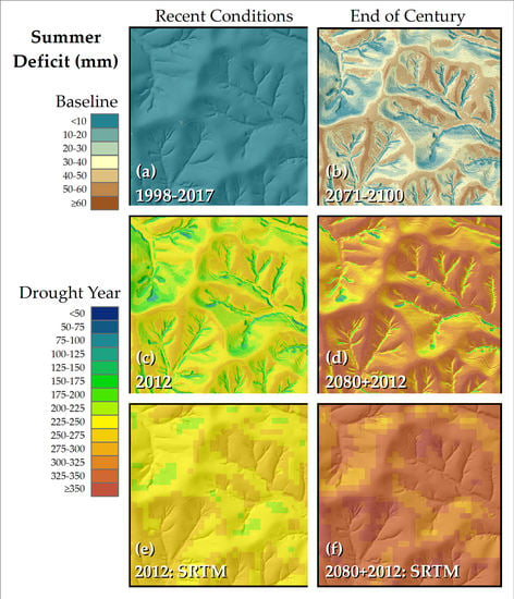
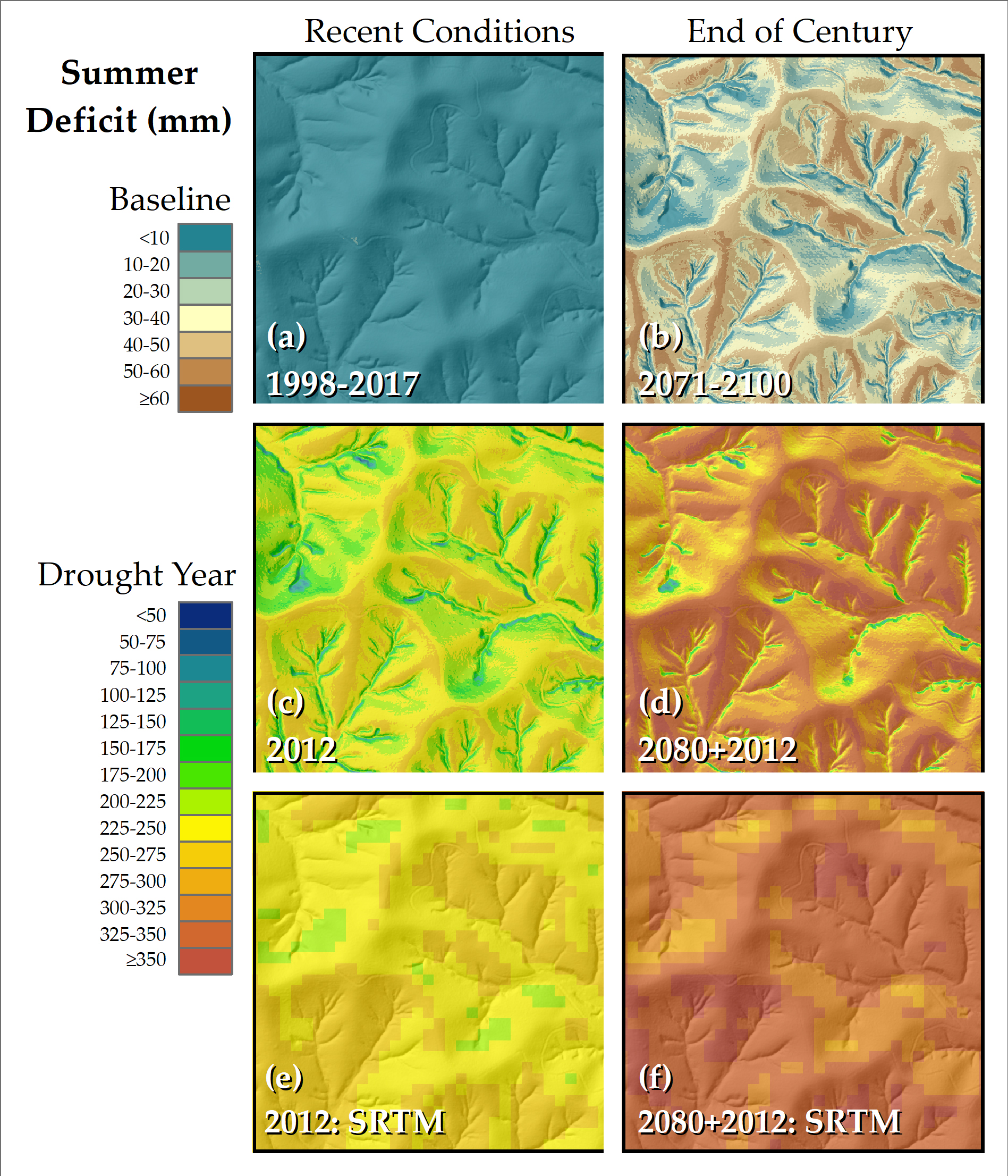
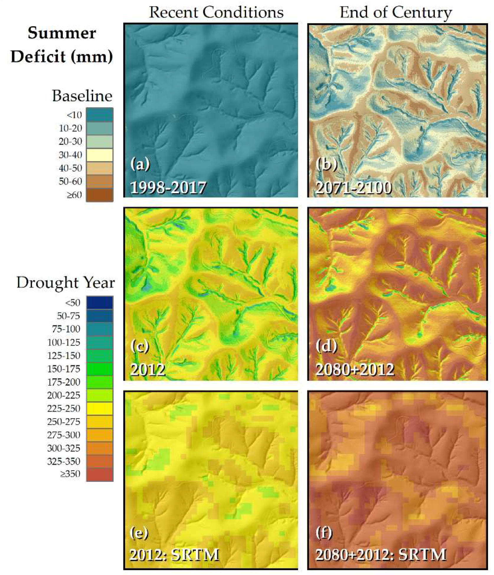
When using average monthly values of temperature, precipitation, and radiation, relatively small summer (JJA) deficit is observed across the study area for the 1998–2017 baseline (Figure 2a; Table 1). Summer deficit represents 1.2% of demand (potential evapotranspiration). With the small summer deficit, average annual surplus is 511 mm, representing 39.4% of annual precipitation. JJA deficits increase significantly in the 2012 drought year (representing 56.5% of demand; Table 1), and a pronounced topographic pattern is evident (Figure 2c). Compared to the LiDAR DEM, mean JJA deficit in 2012 is similar using the SRTM DEM, but the range of values captured across the landscape is greatly reduced (Table 1). Obviously, the coarse-resolution SRTM DEM is unable to capture fine-scale topographic variation (Figure 2e).
Table 2 presents a tally of species comprising ≥1% of all trees ≥30 cm DBH (n = 3137) at Lilly–Dickey Woods. Tallies are presented for canopy (≥30 cm DBH) and subcanopy trees (10–19 cm DBH, n = 3476). Whereas oaks and hickory comprise 73% of trees in the larger size class, their representation decreases in the smaller size class, as does the early successional tulip poplar. In contrast, maples and beech comprise 89% of stems in the smaller size class, but only 20% of stems in the larger size class.
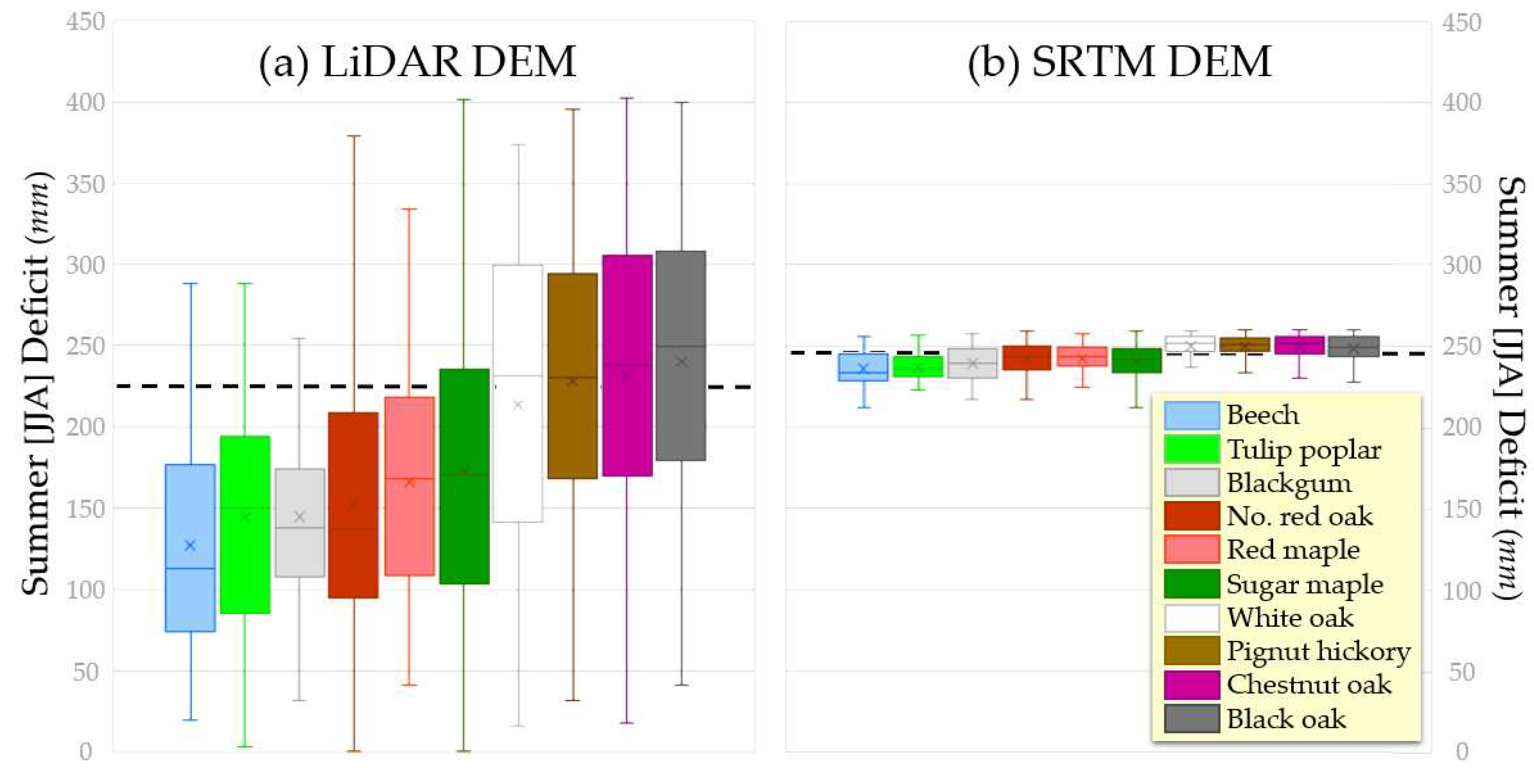
Tree locations were plotted over the water balance grids, and the value of 2012 JJA deficit was extracted for each tree ≥30 cm DBH in the 25-ha forest dynamics plot; the distributions for the most abundant species are presented as box and whisker plots (Figure 3a). Using the LiDAR-derived DEM, individual species evince wide ecological amplitude (i.e., they occur on sites across a range of values), but do segregate according to summer deficit. Notably, beech, tulip poplar, blackgum, northern red oak, red maple, and sugar maple preferentially occur on the more mesic sites, whereas white oak, pignut hickory, chestnut oak, and black oak occur on sites experiencing greater moisture stress. Using the SRTM DEM, the segregation of mesic and more xeric species also emerges, though the range of deficit values is greatly compressed (Figure 3b).
3.3. Water Balance under an RCP8.5 2080s Scenario
Extremely high deficit values were not observed with the 2080s (2071–2100 average) projection (Figure 2b, Table 1), as was also the case with the 1998–2017 baseline scenario. Yet the mean deficit value for the 2080s projection exceeded the maximum value observed under the 1998–2017 baseline. Summer deficit represents 7.6% of demand, and the higher summer deficit under the 2080s projection reduced annual surplus, both in terms of total amount (461 mm) and as a percentage of annual precipitation (32.6%). When the projected changes were applied to 2012 monthly values, extreme deficit conditions are observed (Figure 2d). Summer deficit represents 66.3% of demand, and the mean value is higher than the maximum value observed under the previous scenarios (Table 1). As with the actual 2012 simulation, pockets of more mesic settings are maintained on the landscape using a fine-resolution DEM, but not the SRTM-derived DEM (Figure 2d,f).
4. Discussion
Deficit computed by the Water Balance Toolset correlates highly with the SPEI drought index at a range of sites across the eastern deciduous forest, and demonstrates that the water balance approach is able to capture the drought signal of a site. The correspondence is not surprising, since both measures evaluate the relationship between precipitation (supply) and potential evapotranspiration (demand). A water balance approach additionally accounts for the availability of soil storage, and a previous application demonstrated its ability to capture seasonal patterns recorded by soil moisture probes in North Carolina and Ohio [25]. In contrast to a standard drought index that calculates a single value for a study site, the Water Balance Toolset captures inter-landscape variation, and quantifies both moisture demand and deficit in millimeters of water.
At Lilly–Dickey Woods, a hilly site with moderate relief, the Water Balance Toolset was used to simulate the significant drought year of 2012, since extreme climatic events are likely more critical in defining environmental gradients compared to average conditions [45]. Topographically controlled gradients in moisture conditions were evident: exposed ridges and slopes, with their higher radiation loads, experienced the largest deficits; smaller deficits occurred in more sheltered locations. Trees in the largest size class, which likely established in the 19th century, segregate along these moisture stress gradients. Drought-adapted oak and hickory species preferentially occur on high-deficit sites, while mesic species such as maple and beech are more prominent on low-deficit sites. Thus, water balance modeling was able to capture inter-landscape distribution patterns described for this region: beech and maple dominate the canopy in ravines and on north-facing slopes, while oak and hickory are canopy dominants on ridges and south-facing slopes [3,32,33]. Changes in patterns of abundance along environmental gradients affirms the importance of fine-scale habitat variability in maintaining species diversity under changing climatic conditions.
Outside of the 1998–2017 baseline period, more intense droughts of longer duration have been recorded in the region in the 1930s and 1950s [46], and in the 1880s as inferred from tree-ring reconstructions [31]; these events may have influenced the species distribution of present-day canopy trees at Lilly–Dickey Woods. In contrast, the late 20th century has witnessed a trend of increased moisture availability, and is among the wettest periods in the eastern U.S. in the last 500 years [47,48]; wetter climatic conditions may explain the changing pattern observed in trees that established in the 20th century at Lilly–Dickey Woods. In the smaller size-class, mesic species have expanded into the high-deficit sites, and drought-tolerant species have experienced an overall decline. A similar topographic shift has been reported in neighboring Ohio [9]. There, drought-tolerant species were formerly more abundant across the landscape c. 1800, but now preferentially occur in more restricted topographic settings such as ridges. Mesic species, in contrast, expanded from slopes and valleys into a wider range of topographic settings. Edaphic characteristics also played a role in the observed shifts in Ohio, and individualistic responses may challenge predictions of vegetation response to future climate change. Yet the Ohio and Indiana findings suggest that regional climate change may have altered competitive relationships, such that patterns of abundance have shifted within the landscape. A similar response could be expected with future climate change.
Water-balance projections for Lilly-Dicky Woods derived from the RCP8.5 scenario indicate a dramatic increase in both total deficit, and deficit as a percentage of demand by the end of this century (Table 1). These conditions would favor drought-tolerant species such as oak and hickory, over mesic species such as beech and maple that have been increasing in importance over the 20th century. Water-balance modeling using the LiDAR-based DEM indicated the persistence of more mesic habitat, even under significant drought conditions (Figure 2d). Although reduced in extent, mesic habitat is projected to persist under extreme drought conditions modeled for late century. This is not the case when using the coarse-resolution SRTM DEM (Figure 2f). Mean deficit values were similar with the two DEMs, but the variability about the mean is greatly reduced with SRTM (Table 1); this observation is explained by the fact that the area covered by a single pixel in the SRTM is comprised of over 300 pixels with the LiDAR DEM. If fine-scale pattern is critical for the analysis, a high-resolution DEM is recommended.
The Water Balance Toolset provides a fine-resolution assessment of moisture demand and moisture availability, though users should be aware of certain limitations. For example, to account for availability, the Water Balance Toolset relies on precipitation inputs, and soil available water capacity. Proximity to surface water bodies is not addressed, nor is moisture augmentation from upslope drainage. As the soil dries, its hydraulic conductivity decreases, and topographic control on subsurface drainage is less evident [49,50,51]. During much of the growing season, soil moisture is likely to be below field capacity, and upslope augmentation likely is not a significant influence. If soil moisture is at field capacity, then plants are not experiencing moisture deficit, regardless of upslope augmentation. Since the focus has been on summer conditions, the model also did not account for monthly precipitation carryover as snowpack; a storage detention routine should be implemented if important for the application. To model demand (potential evapotranspiration), the Water Balance Toolset considers temperature and radiation using a monthly time step. Since diurnal variations in temperature are not considered, maximum demand occurs on southern exposures (in the northern hemisphere), since that is where maximum insolation occurs (and modeled potential evapotranspiration is symmetrical about the north–south axis). Yet typically, higher potential evapotranspiration is associated with more westerly aspects because temperatures and vapor pressure deficits are higher in the afternoon when these aspects are receiving the most direct radiation. However, an approach to adjust potential evapotranspiration based on diurnal temperature patterns had minimal influence on summer values for Lilly–Dickey Woods. (The adjustment method is presented on the author’s web page, https://people.ohio.edu/dyer/.)
5. Conclusions
Because it simultaneously incorporates solar energy, available moisture, and their interaction throughout the year, the water balance has utility for a range of ecological applications. Water balance variables have explained broad-scale patterns in species richness [52], decomposition rates [53], and net primary productivity [54]; they have also been used to delineate vegetation associations at global to regional scales [2,17,55]. Available moisture and energy also influence the distribution of tree species at finer scales of analysis, though other variables may assume increasing importance. Since topography influences radiation load and drainage patterns, it results in distinctive vegetation assemblages in upland forest communities. Despite probable individualistic responses to altered conditions, vegetation responses to future climate change are likely to manifest along topographic gradients.
At a central Indiana study site, regional climate projections suggest that within the next 50 years, conditions may favor drought-tolerant species, and curtail mesic species within the landscape. By utilizing downscaled GCM data and fine-resolution LiDAR-derived DEM, the water balance model suggested pockets of mesic habitat may persist in the landscape, even with drought conditions under the harsh RCP8.5 scenario (Figure 2d). This result affirms the critical role for topography in creating microclimates that are distinct from the regional climate, which can serve as microrefugia for species in retreat from the deleterious effects of altered climate [56]. These sites may also serve as stepping stones as species migrate to newly defined ranges [57]. The identification of potential microrefugia is a critical priority for species diversity and conservation efforts in the coming decades [58]. In recent years, high-resolution gridded datasets of climate, soils, and radiation have become increasingly available. The water balance approach presented here highlights the potential for incorporation of fine-scale digital elevation models into regional analyses of moisture relations. The LiDAR-derived DEM employed at Lilly–Dickey Woods enabled the modeling of potential evapotranspiration at 1.5-meter resolution; assessing moisture demand and availability at an “individual tree scale” permits a fine-scale analysis of vegetation response to environmental gradients under different climatic conditions.
Topographic gradients produce varied microclimates, creating habitat diversity within the landscape. Habitat diversity in turn is linked to species richness; indeed, topographic diversity serves as a key element of The Nature Conservancy’s efforts to identify species-diverse areas using abiotic surrogates [59]. This paper presents a GIS-based tool to identify areas with distinctive topoclimates [56], by computing a monthly water balance for all pixels within a study area. The tool requires minimal inputs (monthly temperature, precipitation, and radiation, soil available water capacity, and a digital elevation model), and requires only a basic proficiency with ArcGIS. By incorporating climatic variables, the model enables an assessment of changing conditions, including the interactive effects between moisture demand (temperature, radiation) and availability (precipitation, soil storage). Units of all output grids are expressed as amounts of water (mm), which facilitate ecological interpretation and enable comparisons among sites. Mean deficit computed by the Water Balance Toolset at four sites across the eastern deciduous forest correlated highly with an established drought index, though the strength of the Toolset is its ability to model fine-scale variation within a landscape. Because of its ability to capture fine-scale variation in moisture relationships, the Water Balance Toolset can be useful in exploring species–environment linkages.
Supplementary Materials
The following are available online at https://www.mdpi.com/2072-4292/11/20/2385/s1, Water Balance Toolset for ArcGIS, User Manual.
Funding
This research received funding from the National Park Service, Task Agreement P16AC01753, and the CTFS—ForestGEO Research Grants Program.
Acknowledgments
I very much appreciate the support I received from other researchers: Rich Phillips and Dan Johnson provided tree-survey and ancillary data for Lilly–Dickey Woods, and Scott Robeson provided monthly change estimates for downscaled GCM data. Steve Porter performed the Python coding to automate the Water Balance tool.
Conflicts of Interest
I declare no conflict of interest. The funders had no role in the design of the study; in the collection, analyses, or interpretation of data; in the writing of the manuscript, or in the decision to publish the results.
References
- Lookingbill, T.; Urban, D. An empirical approach towards improved spatial estimates of soil moisture for vegetation analysis. Landsc. Ecol. 2004, 19, 417–433. [Google Scholar] [CrossRef]
- Stephenson, N.L. Climatic Control of Vegetation Distribution: The Role of the Water Balance. Am. Nat. 1990, 135, 649–670. [Google Scholar] [CrossRef]
- Potzger, J.E. Topography and Forest Types in a Central Indiana Region. Am. Midl. Nat. 1935, 16, 212–229. [Google Scholar] [CrossRef]
- Cantlon, J.E. Vegetation and Microclimates on North and South Slopes of Cushetunk Mountain, New Jersey. Ecol. Monogr. 1953, 23, 241–270. [Google Scholar] [CrossRef]
- McCarthy, B.C.; Small, C.J.; Rubino, D.L. Composition, structure and dynamics of Dysart Woods, an old-growth mixed mesophytic forest of southeastern Ohio. For. Ecol. Manag. 2001, 140, 193–213. [Google Scholar] [CrossRef]
- Wolfe, J.N.; Wareham, R.T.; Schofield, H.T. Microclimates and Macroclimate of Neatoma, A Small Valley in Central Ohio; Ohio Biology Survey; The Ohio State University: Columbus, OH, USA, 1949; p. 267. [Google Scholar]
- Hutchins, R.B.; Blevins, R.L.; Hill, J.D.; White, E.H. The influence of soils and microclimate on vegetation of forested slopes in eastern kentucky. Soil Sci. 1976, 121, 234–241. [Google Scholar] [CrossRef]
- Iverson, L.R.; Peters, M.P.; Prasad, A.M.; Matthews, S.N. Analysis of Climate Change Impacts on Tree Species of the Eastern US: Results of DISTRIB-II Modeling. Forests 2019, 10, 302. [Google Scholar] [CrossRef]
- Dyer, J.M.; Hutchinson, T.F. Topography and soils-based mapping reveals fine-scale compositional shifts over two centuries within a central Appalachian landscape. For. Ecol. Manag. 2019, 433, 33–42. [Google Scholar] [CrossRef]
- Palmer, W.C. Meteorological Drought; U.S. Department of Commerce Weather Bureau: Washington, DC, USA, 1965.
- Vicente-Serrano, S.M.; Beguería, S.; López-Moreno, J.I. A Multiscalar Drought Index Sensitive to Global Warming: The Standardized Precipitation Evapotranspiration Index. J. Clim. 2010, 23, 1696–1718. [Google Scholar] [CrossRef] [Green Version]
- Beven, K.J.; Kirkby, M.J. A physically based, variable contributing area model of basin hydrology. Hydrol. Sci. Bull. 1979, 24, 43–69. [Google Scholar] [CrossRef]
- Iverson, L.R.; Dale, M.E.; Scott, C.T.; Prasad, A. A Gis-derived integrated moisture index to predict forest composition and productivity of Ohio forests (U.S.A.). Landsc. Ecol. 1997, 12, 331–348. [Google Scholar] [CrossRef]
- Iverson, L.R.; Peters, M.P.; Bartig, J.L.; Rebbeck, J.; Hutchinson, T.F.; Matthews, S.N.; Stout, S. Spatial modeling and inventories for prioritizing investment into oak-hickory restoration. For. Ecol. Manag. 2018, 424, 355–366. [Google Scholar] [CrossRef]
- Mohamedou, C.; Korhonen, L.; Eerikäinen, K.; Tokola, T. Using LiDAR-modified topographic wetness index, terrain attributes with leaf area index to improve a single-tree growth model in south-eastern Finland. Forestry 2019, 92, 253–263. [Google Scholar] [CrossRef]
- Mather, J.R. The Climatic Water Budget in Environmental Analysis; D.C. Heath and Company: Lexington, MA, USA, 1978; p. 239. [Google Scholar]
- Stephenson, N.L. Actual evapotranspiration and deficit: Biologically meaningful correlates of vegetation distribution across spatial scales. J. Biogeogr. 1998, 25, 855–870. [Google Scholar] [CrossRef]
- Crimmins, S.M.; Dobrowski, S.Z.; Greenberg, J.; Abatzoglou, J.T.; Mynsberge, A.R. Changes in Climatic Water Balance Drive Downhill Shifts in Plant Species’ Optimum Elevations. Science 2011, 331, 324–327. [Google Scholar] [CrossRef]
- Harsch, M.A.; HilleRisLambers, J. Climate Warming and Seasonal Precipitation Change Interact to Limit Species Distribution Shifts across Western North America. PLoS ONE 2016, 11, e0159184. [Google Scholar] [CrossRef]
- Monteith, J.L. Evaporation and environment. In The State and Movement of Water in Living Organisms, Proceedings of the 19th Symposium of the Society for Experimental Biology; Fogg, G.E., Ed.; Cambridge University Press: New York, NY, USA, 1965; pp. 205–234. [Google Scholar]
- Allen, R.G.; Pereira, L.S.; Raes, D.; Smith, M. Crop Evapotranspiration—Guidelines for Computing Crop Water Requirements; FAO Irrigation and Drainage Paper 56; Food and Agricultural Organization of the United Nations: Rome, Italy, 1998; p. 326. [Google Scholar]
- Fua, H.; Tajchmana, S.J.; Kochenderferb, J.N. Topography and radiation exchange of a mountainous watershed. J. Appl. Meteorol. 1995, 34, 890–901. [Google Scholar] [CrossRef]
- Turc, L. Evaluation des besoins en eau d’irrigation, évapotranspiration potentielle, formule climatique simplifie et mise a jour. Ann. Agron. 1961, 12, 13–49. [Google Scholar]
- American Society of Civil Engineers. Evapotranspiration and Irrigation Water Requirements; American Society of Civil Engineers: New York, NY, USA, 1990; p. 332. [Google Scholar]
- Dyer, J.M. Assessing topographic patterns in moisture use and stress using a water balance approach. Landsc. Ecol. 2009, 24, 391–403. [Google Scholar] [CrossRef]
- Gale, M.R.; Grigal, D.F. Vertical root distributions of northern tree species in relation to successional status. Can. J. For. Res. 1987, 17, 829–834. [Google Scholar] [CrossRef]
- Jackson, R.B.; Canadell, J.; Ehleringer, J.R.; Mooney, H.A.; Sala, O.E.; Schulze, E.D. A global analysis of root distributions for terrestrial biomes. Oecologia 1996, 108, 389–411. [Google Scholar] [CrossRef] [PubMed]
- Yeakley, J.A.; Swank, W.T.; Swift, L.W.; Hornberger, G.M.; Shugart, H.H. Soil moisture gradients and controls on a southern Appalachian hillslope from drought through recharge. Hydrol. Earth Syst. Sci. 1998, 2, 41–49. [Google Scholar] [CrossRef] [Green Version]
- Florinsky, I.; Eilers, R.; Manning, G.; Fuller, L.; Florinsky, I. Prediction of soil properties by digital terrain modelling. Environ. Model. Softw. 2002, 17, 295–311. [Google Scholar] [CrossRef]
- Soil Survey Staff, Natural Resources Conservation Service, United States Department of Agriculture. Web Soil Survey. Available online: https://websoilsurvey.sc.egov.usda.gov/ (accessed on 20 March 2018).
- Maxwell, J.T.; Harley, G.L. Increased tree-ring network density reveals more precise estimations of sub-regional hydroclimate variability and climate dynamics in the Midwest, USA. Clim. Dyn. 2017, 49, 1479–1493. [Google Scholar] [CrossRef]
- Braun, E.L. Deciduous Forests of Eastern North America; Blakiston: Philadelphia, PA, USA, 1950; p. 596. [Google Scholar]
- Homoya, M.A.; Abrell, D.B.; Aldrich, J.A.; Post, T.W. The natural regions of Indiana. Proc. Indiana Acad. Sci. 1985, 94, 245–268. [Google Scholar]
- Sengupta, M.; Xie, Y.; Lopez, A.; Habte, A.; Maclaurin, G.; Shelby, J. The National Solar Radiation Data Base (NSRDB). Renew. Sustain. Energy Rev. 2018, 89, 51–60. [Google Scholar] [CrossRef]
- Daly, C.; Halbleib, M.; Smith, J.I.; Gibson, W.P.; Doggett, M.K.; Taylor, G.H.; Curtis, J.; Pasteris, P.P. Physiographically sensitive mapping of climatological temperature and precipitation across the conterminous United States. Int. J. Clim. 2008, 28, 2031–2064. [Google Scholar] [CrossRef]
- Jackson, S.T.; Betancourt, J.L.; Booth, R.K.; Gray, S.T. Ecology and the ratchet of events: Climate variability, niche dimensions, and species distributions. Proc. Natl. Acad. Sci. USA 2009, 106, 19685–19692. [Google Scholar] [CrossRef] [Green Version]
- Berdanier, A.B.; Clark, J.S. Multiyear drought-induced morbidity preceding tree death in southeastern U.S. forests. Ecol. Appl. 2016, 26, 17–23. [Google Scholar] [CrossRef]
- Climate at A Glance: Divisional Time Series. Available online: https://www.ncdc.noaa.gov/cag/ (accessed on 25 March 2017).
- Hamlet, A.F.; Byun, K.; Robeson, S.M.; Widhalm, M.; Baldwin, M. Impacts of climate change on the state of Indiana: Ensemble future projections based on statistical downscaling. Clim. Chang. 2019, 1–15. [Google Scholar] [CrossRef]
- Van Vuuren, D.P.; Edmonds, J.; Kainuma, M.; Riahi, K.; Thomson, A.; Hibbard, K.; Hurtt, G.C.; Kram, T.; Krey, V.; Lamarque, J.F.; et al. The representative concentration pathways: An overview. Clim. Chang. 2011, 109, 5–31. [Google Scholar] [CrossRef]
- Sanford, T.; Frumhoff, P.C.; Luers, A.; Gulledge, J. The climate policy narrative for a dangerously warming world. Nat. Clim. Chang. 2014, 4, 164–166. [Google Scholar] [CrossRef]
- Design Your Own CSV File of MACA Point Data. Available online: https://climate.nkn.uidaho.edu/MACA/ (accessed on 13 March 2019).
- SPEI: Calculation of the Standardised Precipitation–Evapotranspiration Index. Available online: https://CRAN.R-project.org/package=SPEI (accessed on 17 August 2019).
- Hargreaves, G.H. Defining and Using Reference Evapotranspiration. J. Irrig. Drain. Eng. 1994, 120, 1132–1139. [Google Scholar] [CrossRef]
- Hawthorne, S.; Miniat, C.F. Topography may mitigate drought effects on vegetation along a hillslope gradient. Ecohydrology 2018, 11, e1825. [Google Scholar] [CrossRef]
- Maxwell, J.T.; Harley, G.L.; Robeson, S.M. On the declining relationship between tree growth and climate in the Midwest United States: The fading drought signal. Clim. Chang. 2016, 138, 127–142. [Google Scholar] [CrossRef]
- Roque-Malo, S.; Kumar, P. Patterns of change in high frequency precipitation variability over North America. Sci. Rep. 2017, 7, 10853. [Google Scholar] [CrossRef]
- Pederson, N.; D’Amato, A.W.; Dyer, J.M.; Foster, D.R.; Goldblum, D.; Hart, J.L.; Hessl, A.E.; Iverson, L.R.; Jackson, S.T.; Martin-Benito, D.; et al. Climate remains an important driver of post-European vegetation change in the eastern United States. Glob. Chang. Biol. 2015, 21, 2105–2110. [Google Scholar] [CrossRef]
- Grayson, R.B.; Western, A.W.; Blöschl, G. Scaling of Soil Moisture: A Hydrologic Perspective. Annu. Rev. Earth Planet. Sci. 2002, 30, 149–180. [Google Scholar] [Green Version]
- Chamran, F.; Gessler, P.E.; Chadwick, O.A. Spatially Explicit Treatment of Soil-Water Dynamics along a Semiarid Catena. Soil Sci. Soc. Am. J. 2002, 66, 1571–1583. [Google Scholar] [CrossRef]
- Park, S.; Van De Giesen, N. Soil–landscape delineation to define spatial sampling domains for hillslope hydrology. J. Hydrol. 2004, 295, 28–46. [Google Scholar] [CrossRef]
- Currie, D.J. Energy and Large-Scale Patterns of Animal-and Plant-Species Richness. Am. Nat. 1991, 137, 27–49. [Google Scholar] [CrossRef]
- Dyer, M.L.; Meentemeyer, V.; Borg, B. Apparent controls of mass loss rate of leaf litter on a regional scale: Litter quality versus climate. Scand. J. For. Res. 1990, 5, 311–323. [Google Scholar] [CrossRef]
- Rosenzweig, M.L. Net Primary Productivity of Terrestrial Communities: Prediction from Climatological Data. Am. Nat. 1968, 102, 67–74. [Google Scholar] [CrossRef]
- Hogg, E.H. (Ted) Climate and the southern limit of the western Canadian boreal forest. Can. J. For. Res. 1994, 24, 1835–1845. [Google Scholar] [CrossRef]
- Dobrowski, S.Z. A climatic basis for microrefugia: The influence of terrain on climate. Glob. Chang. Biol. 2011, 17, 1022–1035. [Google Scholar] [CrossRef]
- Hannah, L.; Flint, L.; Syphard, A.D.; Moritz, M.A.; Buckley, L.B.; McCullough, I.M. Fine-grain modeling of species’ response to climate change: Holdouts, stepping-stones, and microrefugia. Trends Ecol. Evol. 2014, 29, 390–397. [Google Scholar] [CrossRef]
- Keppel, G.; Mokany, K.; Wardell-Johnson, G.W.; Phillips, B.L.; Welbergen, J.A.; Reside, A.E. The capacity of refugia for conservation planning under climate change. Front. Ecol. Environ. 2015, 13, 106–112. [Google Scholar] [CrossRef]
- Beier, P.; Sutcliffe, P.; Hjort, J.; Faith, D.P.; Pressey, R.L.; Albuquerque, F. A review of selection-based tests of abiotic surrogates for species representation. Conserv. Biol. 2015, 29, 668–679. [Google Scholar] [CrossRef] [Green Version]
Figure 1.
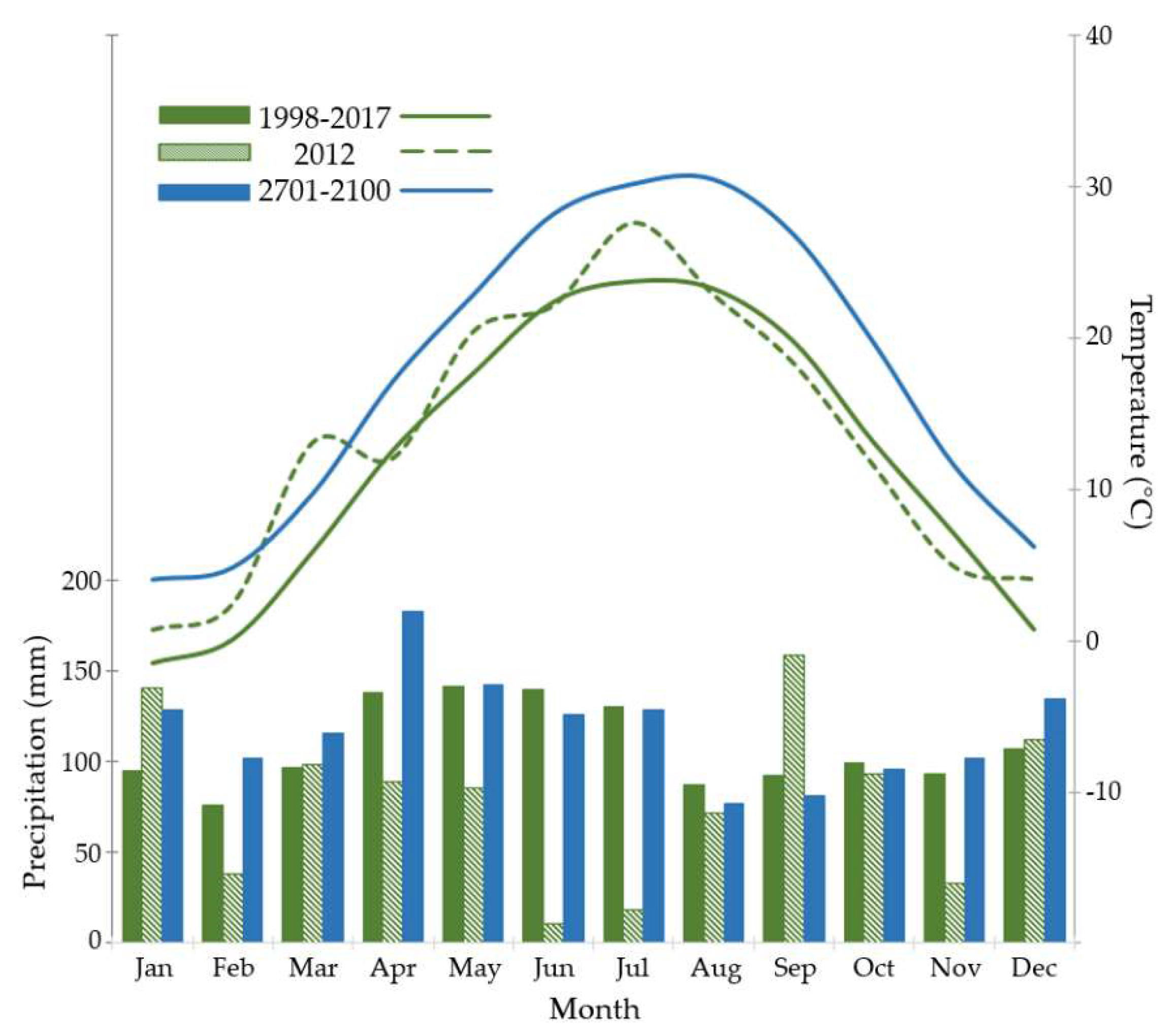
Climate diagram for Lilly–Dickey Woods. Bars represent precipitation and lines represent temperature, for average conditions observed 1998–2017, the drought year 2012, and projected for 2071–2100. Annual precipitation was 949 mm in 2012, but averaged 1296 mm during 1998–2017; average annual precipitation was projected to increase to 1416 mm during 2071–2100. Recent climate data from PRISM data sets, which were projected for future conditions [39] as described in text.
Figure 1.
Climate diagram for Lilly–Dickey Woods. Bars represent precipitation and lines represent temperature, for average conditions observed 1998–2017, the drought year 2012, and projected for 2071–2100. Annual precipitation was 949 mm in 2012, but averaged 1296 mm during 1998–2017; average annual precipitation was projected to increase to 1416 mm during 2071–2100. Recent climate data from PRISM data sets, which were projected for future conditions [39] as described in text.

Figure 2.
Modeled summer (JJA) water deficit for Lilly–Dickey Woods. Depicted area measures 900 m × 900 m, centered on the 25-ha ForestGEO plot. Left panels represent simulations of recent observed climatic conditions, right panels are comparable simulations for end-of-21st century climatic projections derived from the RCP8.5 radiative forcing scenario: (a) baseline conditions using average monthly values, 1998–2017; (b) baseline conditions with projected changes for 2071–2100 (“2080”); (c) drought year 2012; (d) projected future changes applied to 2012 values; (e) same historical simulation as (c) using NASA Shuttle Radar Topography Mission (SRTM) Digital Elevation Model (DEM); (f) same scenario as (d) using SRTM DEM. Light Detection and Ranging (LiDAR)-derived DEM used for (a–d); its hillshade projected over all images.

Figure 3.
Box and whisker plots illustrating distribution of trees ≥30 cm DBH at Lilly–Dickey Woods with respect to summer 2012 water deficit, computed using (a) LiDAR-derived DEM, and (b) SRTM DEM. Dashed line represents average deficit value for the grid (Figure 2c,e). The top and bottom of each box represents the upper and lower quartiles, X represents the mean, and the horizontal line the median.


Table 1.
Descriptive statistics for summer [JJA] water deficit, precipitation (P), and potential evapotranspiration (PET) (units = mm), for water balance simulations depicted in Figure 2. The first three simulations utilize recent observed climatic conditions, the last three are based upon end-of-21st century climatic projections derived from the RCP8.5 radiative forcing scenario.
| Figure 2 Grid | Mean Deficit | Standard Deviation | Min | Max | P | Mean PET | Deficit as Percentage of PET | |
|---|---|---|---|---|---|---|---|---|
| 1998–2017 | (a) | 4 | 3 | 0 | 10 | 357 | 373 | 1.2 |
| 2012 | (c) | 226 | 27 | 63 | 266 | 100 | 400 | 56.5 |
| 2012: SRTM | (e) | 246 | 11 | 205 | 261 | 100 | 421 | 58.3 |
| 2071–2100 (2080) | (b) | 33 | 13 | 0 | 54 | 332 | 429 | 7.6 |
| 2080 + 2012 | (d) | 305 | 39 | 63 | 356 | 91 | 461 | 66.3 |
| 2080 + 2012: SRTM | (f) | 333 | 15 | 274 | 354 | 91 | 484 | 68.7 |
Table 2.
Dominant canopy trees (≥1% of all trees ≥30 cm) on Lilly–Dickey Woods forest dynamics plot. Tally and percentages by size class (≥30 cm diameter at breast height (DBH), n = 3137, and 10–19 cm DBH, n = 3476).
Table 2.
Dominant canopy trees (≥1% of all trees ≥30 cm) on Lilly–Dickey Woods forest dynamics plot. Tally and percentages by size class (≥30 cm diameter at breast height (DBH), n = 3137, and 10–19 cm DBH, n = 3476).
| Species | Common Name | ≥30 cm DBH | 10–19 cm DBH | ||
|---|---|---|---|---|---|
| n | Percent | n | Percent | ||
| Acer rubrum | Red maple | 39 | 1.2 | 318 | 9.1 |
| Acer saccharum | Sugar maple | 519 | 16.5 | 2160 | 62.1 |
| Carya glabra | Pignut hickory | 155 | 4.9 | 67 | 1.9 |
| Fagus grandifolia | American beech | 70 | 2.2 | 610 | 17.5 |
| Liriodendron tulipifera | Tulip poplar | 35 | 1.1 | 4 | 0.1 |
| Nyssa sylvatica | Blackgum | 43 | 1.4 | 72 | 2.1 |
| Quercus alba | White oak | 194 | 6.2 | 20 | 0.6 |
| Quercus montana | Chestnut oak | 1551 | 49.4 | 79 | 2.3 |
| Quercus rubra | Northern red oak | 176 | 5.6 | 1 | <0.1 |
| Quercus velutina | Black oak | 202 | 6.4 | 2 | 0.1 |
© 2019 by the author. Licensee MDPI, Basel, Switzerland. This article is an open access article distributed under the terms and conditions of the Creative Commons Attribution (CC BY) license (http://creativecommons.org/licenses/by/4.0/).
Share and Cite
MDPI and ACS Style
Dyer, J.M. A GIS-Based Water Balance Approach Using a LiDAR-Derived DEM Captures Fine-Scale Vegetation Patterns. Remote Sens. 2019, 11, 2385. https://doi.org/10.3390/rs11202385
AMA Style
Dyer JM. A GIS-Based Water Balance Approach Using a LiDAR-Derived DEM Captures Fine-Scale Vegetation Patterns. Remote Sensing. 2019; 11(20):2385. https://doi.org/10.3390/rs11202385
Chicago/Turabian StyleDyer, James M. 2019. "A GIS-Based Water Balance Approach Using a LiDAR-Derived DEM Captures Fine-Scale Vegetation Patterns" Remote Sensing 11, no. 20: 2385. https://doi.org/10.3390/rs11202385
Note that from the first issue of 2016, this journal uses article numbers instead of page numbers. See further details here.