Frost Damage Assessment in Wheat Using Spectral Mixture Analysis

Abstract

Frost damage to broadacre crops can cause up to an 85% loss in productivity. Although growers have few options for crop protection from frost, a rapid method for assessing frost-induced sterility would allow for timely management decisions (e.g., cutting for hay and altering marketing strategies). Spectral mixture analysis (SMA) has shown success in mapping landscape components and was used with hyperspectral data collected on the canopy, heads, and leaves of wheat at different sites to determine if this could quantify frost damage. Spectral libraries were assembled from canopy components collected from local field sites to generate spectral libraries for SMA from which a series of fraction sets was derived. The frost (Fr) fraction was then used to estimate final yield as a means of measuring frost damage. The best-fitting Fr fractions to yield were derived from the same data set as the source Fr spectra, and these ranged over R² = 0.58–0.75 at the canopy scale. It was clear that spectral signatures need to be collected at scale to assess frost damage. While Fr fractions were able to estimate yield there was no “universal” endmember set from which a Fr fraction could be derived. The normalized difference vegetation index (NDVI) was not able to estimate frost damage consistently. Future work requires determining whether there is a “universal” set of endmembers and a minimum set of targeted wavebands that could lead to multispectral instruments for frost assessment for use in ground and aerial sensors.

1. Introduction

Frost damage in broadacre crop production has been found to cause significant economic losses in cereals, oilseeds, and pulses [1,2,3]. Losses in productivity of up to 85% have been reported after post-head-emergence frost in both the U.S. and Australia [4,5,6]. In Australia in particular, frost damage is estimated to cost the agriculture sector between $120 and $700 million annually [7]. Additional economic losses can be incurred when adopting inappropriate risk minimization strategies for avoiding frost damage.

Radiation frosts occur on clear nights when energy loss by longwave radiation to space is greater from the upper layers of the crop compared with that occurring at the soil surface, causing a net chilling of the canopy [8]. Under climate change scenarios it is expected that the impact of radiation frost may increase in the short term due to both drier atmospheric conditions from greater incidence of clear nights and more rapid development of crops inducing earlier flowering when the frost risk is higher [9]. Moreover, frost severity is spatially variable across regions and position in the landscape, which translates to frost damage in crops being highly variable at both the inter- and intra-field scales.

Damage to wheat from frost has been observed at all stages of growth, from seedlings through to maturity, although the greatest potential damage to crops such as wheat is during ear emergence and early anthesis [10,11]. During these stages, frost can result in the death of anthers and embryos [12], causing the sterility of florets and whole spikelets [13,14]. Visible symptoms may include bleaching of the awns, or anthers which become pale yellow or white and shriveled, and over time, grain will not form in frosted florets. Frost damage during grain filling is also difficult to assess, with damage generally thought to occur on the attachment between the grain and the ear [15]. However, damage to the supporting stem or grain will result in discolored grains, which may be shrunken, water soaked, or hollow. Frost during grain filling may also result in the death of partially filled grains. Together these impacts can manifest as reduced grain weight and/or small, shriveled, shrunken, and blistered appearances [12]. Frost occurring during the reproductive phase causes a largely nonrecoverable reduction in grain set and yield potential due to the death of anthers and embryos [12].

Limited research using remote sensing methods has shown some success in detecting plant and crop damage. The authors of [16] quantified visual frost damage in oats using a classified digital camera, and in [17] the authors found that leaves from wheat plants that had been subjected to frost exhibited changes in reflectance in the ranges 500–680 nm and 730–740 nm. The authors of [18] demonstrated that for potted wheat seedlings, frost exposure caused decreases in both total reflectance (400–1000 nm) and in the green and near-infrared regions, as well as an increase in the red and a concomitant shift in the red-edge toward longer wavelengths. For wheat, the spectral indices photochemical reflectance index (PRI) and normalized difference vegetation index (NDVI) showed significant relationships with cold load [19].

While not a solution to minimizing frost damage, a rapid and early detection method for assessing frost-induced sterility within a field would allow for timely management decisions, including cutting for hay, reducing inputs, altering grain marketing strategies, and, in general, more informed harvesting logistics [20]. Temperature measurements can be used as a guide to determine whether crops should be assessed for post-head-emergence frost damage, which could be followed up with spectral assessments. However, the identification of specific areas within a field that have been impacted currently requires visual examination for differences in tone or color, vegetation limpness, or stunted grain formation. Inspection of individual frost-affected plants may reveal bleached, shriveled, or dwarfed florets; pale green or white rings around the peduncle; a crimped, cracked, and/or blistered peduncle base; and darkening of damaged areas. These visual clues provide an important step towards empirically measuring and detecting frost damage in broadacre wheat cropping systems. However, there is generally large spatial variation in temperature within a canopy, both vertically and horizontally [21], which may result in damage that cannot be identified when visually scanning vast areas.

For several decades, remote sensing techniques have been used to examine a range of crop characteristics, with some studies more specifically showing the potential use of both vegetation indices and florescence measures for detecting canopy-level frost damage [19,20]. While these two studies provide the foundation on which a body of evidence can be built, further research is required to identify the most appropriate remote sensing techniques for characterizing the spectral response of wheat to frost.

Other techniques based on hyperspectral data might be able to quantify frost damage despite the complexity of factors that appear in assessing frost damage, including the plant component, growth stage, degree of damage, and, potentially, the variety [22]. In vegetation studies, hyperspectral data have been shown to be useful for quantifying a range of biotic and abiotic stresses, including crop nitrogen [23], pests [24,25], nutrient deficiencies [26], and air pollution [27]. To derive useful information from hyperspectral data, appropriate analysis techniques need to be applied. One of these, spectral mixture analysis (SMA), is a physical modelling technique used to quantify the proportion of material within a scene [28] and has become widely used ([29] and references therein) to map subpixel fractions. Because canopies are mixes of many components (leaves of various colors, stems, soils, flowers, fruiting parts, etc.) and each of these has its own spectra, canopy spectra are, by their nature, mixtures of these spectral components. Isolating a particular spectral “signal” from this mixture requires measuring the various spectral components (called endmembers, EMs) in the scene and using spectral unmixing techniques to isolate and quantify the component of interest—in this case, frost damage.

Given this complexity of plant and canopy response to frost, it was proposed that hyperspectral data collected from wheat canopies could provide information to capture a frost “signal”. Combined with spectral mixture analysis, this paper reports a meta-analysis of data collected across three site-years in Australia between 2006 and 2016 to determine if frost damage could be quantified in wheat canopies. Selecting data across sites and years provided an opportunity to test whether the technique could be broadly applied. To guide this analysis, we considered the following questions:

• Can a core or “fixed” set of endmembers (EMs) be identified that can be used to unmix a range of data sets collected from different sites and times, allowing for assessment of frost damage?
• Can frost fractions derived from spectral mixture analysis be used to map frost damage in wheat using yield as a measure of frost damage?

2. Materials and Methods

This research utilized a meta-analysis methodology [30], across three site-years from 2006, 2015, and 2016, to examine the spectral response of frost in wheat canopies and plant components across different varieties in Australian wheat-growing regions. Hyperspectral reflectance data were acquired with frost observations to indicate the presence of frost damage. The data were compiled to develop spectral libraries providing a spectral reference for each site. The spectral libraries were then used in a meta-analysis of all data sets using SMA to assess frost damage in the canopy, wheat heads, and leaves. The frost trials, spectrometer measurements, spectral library development, and subsequent SMA are described below. Using multiple data sets at different locations and times allowed for assessing the complexity of frost and potential differences in the frost “signal”.

2.1. Field Experiments

As noted above, data were collected across three trials in Australia’s southern wheat-growing regions. In the first trial, wheat (Triticum aestivum L., cv. Chara) was sown at the Agriculture Victoria Plant Breeding Centre located near Horsham, Victoria, Australia (−36.741°, 142.104°) in 2006 (PBC2006). To measure yield, plants were cut at ground level (0.4 m²) at maturity from directly under the sensor view. These were dried at 40 °C, threshed, and the grain weighed [31].

As a result of systematic visual examinations [32,33], frost damage was identified in several research plots on 24 October 2006 at anthesis (DC65, [34]). Minimum air temperatures were recorded at 1.2 m and were −1.7, −0.5, and −1.4 °C on 10, 16, and 22 October, respectively. Spectral data were acquired from plots and identified as frost (Fr) or non-frost (NFr) damaged. Frost damage was assessed visually with white heads or portions [35,36] indicating damage. The sensor was positioned 1.5 m above the canopy, resulting in a diameter of approximately 0.7 m at the top of the canopy. NFr plots were considered reference plots but not “controls” in a statistical sense [37], as they were open to the environment but did not exhibit frost damage. The spectral information from non-frosted areas was excluded from the SMA as it was used as reference EMs.

The second trial formed part of a larger research project conducted at Kewell, Victoria (−36.500°, 142.367°) in 2015 (Kewell), [20], which was also sown to wheat (Triticum aestivum L., cv. Wallup). Frost was observed following two natural frost events between heading and anthesis. Minimum air temperatures at 1.2 m (recorded at five-minute intervals) were −1.5 and −2.18 °C for 23 and 29 September, respectively. Spectral measurements were collected across a transect ranging from no visible signs of frost damage to significant frost damage. Spectral data were collected just past anthesis at growth stage DC71–75 on 13 October 2015. Three spectra were collected at each of 31 locations along the transect, with measurements averaged to represent the mean spectrum at each transect point. For the purposes of selecting representative spectral signatures of frosted and non-frosted plants, the median of the three spectra at the beginning of the transect was calculated to represent non-frosted plants (NFr) and the median of the last three spectra was calculated to reflect frosted plants (Fr). At maturity, plant samples were cut from each sensor measurement location (1 m²) at ground level, dried at 40 °C, and threshed for grain to assess yield [20].

Finally, an experiment was conducted in plots sown to wheat (Triticum aestivum L., cv. Yitpi) at the Agriculture Victoria Plant Breeding Centre located near Horsham, Victoria, Australia −36.745°, 142.115°) in 2016 (PBC2016, PBC2016Heads, PBC2016Leaves) [19] with the objective of imposing frost using custom-built chambers on plots sown to wheat. Frost was imposed in two experiments at heading (DC55, ‘H’) and anthesis (DC65, ‘A’) on 24 October and 3 November 2016, respectively. Spectral data were collected on these dates and on 11 November 2016 (DC71–75) after the frost treatments were imposed. Control plots which were open air, where no imposed frosts were applied, were not exposed to any natural frost events in this season; thus, they were considered true controls, unlike those in the Kewell and PBC2006 data sets. The spectra from the control plots were used to develop the NFr EMs but excluded from the yield regression analysis. The canopy-level measurements were collected at 40 cm above the canopy (24 October and 3 November) and 15 cm above the canopy on 11 November, while heads and leaves (collected on 3 November 2016) were measured using a leaf clamp with an internal light source connected to the spectrometer. There were three target data sets derived from this site-year: PBC2016 (canopy), PBC2016Heads, and PBC2016Leaves. At maturity, plants were hand-harvested from 0.24 m² quadrats, and samples were oven-dried at 40 °C then threshed to remove grain for yield assessment [19].

At the heading and anthesis stages, sub-zero temperatures were imposed to test the impact of frost damage on the growth and yield of wheat. The experiment was fully replicated, and the methods are described in detail in [19]. At the two experimental times (‘H’ and ‘A’) different severities and timings of the frost were part of the treatments imposed. In this study, the dataset for the canopy comprised spectral data collected for the ‘H’ experiment on 3 November, 11–13 days after imposed frost, and for the ‘A’ experiment on 11 November, 9–11 days after imposed frost. In the ‘H’ experiment, the degree of cold was enough to cause severe damage to the plants and there was no yield, while in the ‘A’ experiment, the cold load imposed induced much less frost damage and yield was measured.

2.2. Reflectance Measurements

All spectra used for the meta-analysis presented here were collected with the same spectrometer (ASD Field Spec Full Range (FR), Malvern PANalytical, Longmont, Colorado) (350–2500 nm), using an unfiltered sensor with a 25° field of view. For each site, spectra were calibrated to reflectance on the day of acquisition with a 99% Spectralon^TM reference panel measured at frequent intervals to account for changes in irradiance. Spectra were collected at the canopy, head, and leaf scales to represent canopy variability as input for mixture analysis. For the 2016 experiment described below, a leaf clamp was used to measure spectra from wheat leaves and heads.

Spectra were resampled to 2 nm intervals for the regions 400–1818 and 1938–2400 nm and were subsequently used in the analysis. Wavelengths below 400 nm were excluded, as were those in the range 1820–1936 nm and greater than 2400 nm, as these are regions where the atmosphere strongly absorbs energy, leading to poor signal strength. In addition, spectra were smoothed using an 8 nm mean window to remove any fine-scale spurious data.

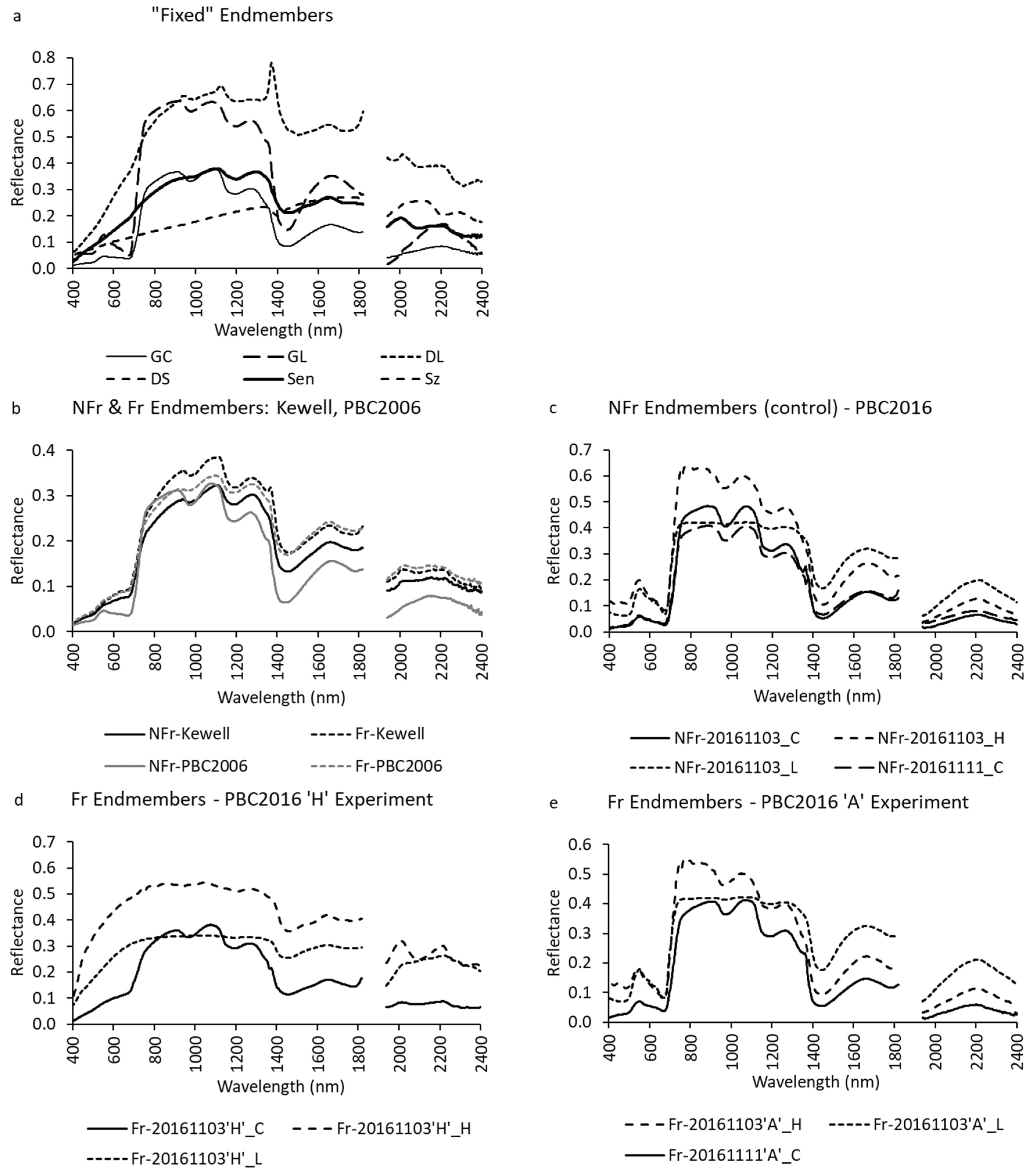
2.3. Spectral Libraries and Endmembers

Endmembers were created from the field-collected spectral data by calculating the median of several reflectance measurements (

Table 1. Libraries, endmembers (EM), EM spectra, and number of spectra used to create each EM for spectral mixture analysis (number in parentheses for first occurrence of EM). All libraries contained the same spectra for senescent canopy (Sen), dead leaf (DL), dry soil (DS) and shade (zero values) (Sz) ¹ (Figure 1a). A single green canopy (GC) or green leaf (GL) spectrum (Figure 1a) was used in a library depending on the scale of measurement. The presence of non-frosted canopy (NFr) and frosted canopy (Fr) EMs varied across libraries as noted (Figure 1b–e). ‘A’ and ‘H’ in names refer to heading and anthesis experiments, respectively. Spectra were derived from the data sets noted (see text for more detail): K = Kewell, P06 = PBC2006, P161103 = PBC2016 3 Nov, P161111 = PBC2016 11 Nov.

Library Number	Library Name	Data Set with EM Spectra, EM Name (no. Spectra to Create EM)
		Kewell 2	PBC2006 3	PBC2016 4
1	Kewell canopy	NFr-K (9), Fr-K (9)	GC (2), Sen (2), DL (2), DS (4)
2	PBC2006 canopy		GC, Sen, DL, DS, NFr-P06 (2), Fr-P06 (2)
3	Kewell leaf	NFr-K, Fr-K	GL (9), Sen, DL, DS
4	PBC2006 leaf		GL, Sen, DL, DS, NFr-P06, Fr-P06
5	PBC2016_’A’ heads		GL, Sen, DL, DS	NFr-P161103_H (20), Fr-P161103′A’_H (5)
6	PBC2016_’A’ leaves		GL, Sen, DL, DS	NFr-P161103_L (20), Fr-P161103′A’_L (5)
7	PBC2016_’A’ canopy		GC, Sen, DL, DS	NFr-P161111_C (20), Fr-P161111′A’_C (5)
8	PBC2016_’H’ canopy		GC, Sen, DL, DS	NFr-P161103_C (12), Fr161103′H’_C (3)
9	PBC2016_’H’ heads		GL, Sen, DL, DS	NFr-P161103_H, Fr-P161103′H’_H
10	PBC2016_’H’ leaves		GL, Sen, DL, DS	NFr-P161103_L, Fr-P161103′H’_L

¹ The shade (Sz) spectrum was all zeros and was included in all libraries and mixture analyses; Figure 1a. ² Kewell: Spectra measured just after heading (DC71–75) on 13 Oct 2015. NFr and Fr collected at either end of a transect from NFr to Fr damaged canopy; Figure 1b. ³ PBC 2006: GC, GL, DL, and DS spectra collected on 26 Oct 2006 (at heading, DC65) and Sen spectra collected on 8 Dec 2006 (harvest, DC90) from the non-frosted plot. Fr (Fr-P06) and NFr (NFr-P06) spectra collected on 24 Oct 2006 from plots with visible frost and nearby non-frost-damaged areas; Figure 1a. ⁴ PBC 2016: The NFr spectra were collected from control plots on 3 Nov (P161103) or 11 Nov (P161111) from heads (H), leaves (L), or canopy (C). Fr spectra were collected from frost-imposed treatments from the heading (‘H’) or anthesis (‘A’) experiments; Figure 1c–e.

) from each target. Seven EMs were selected to build each library as these were considered representative of the relevant canopy components. Ten libraries were assembled to test hypotheses for the ability of the analysis to isolate a frost fraction to estimate yield based on spectra collected at the canopy, head, and leaf scales. The seven EMs, their source data set, and library compositions are presented in Table 1. The seven EM types were green (canopy (GC) or green leaf (GL)), dead leaf (DL), dry soil (DS), senescent canopy (Sen), shade (Sz) (Figure 1a), non-frosted canopy (NFr), and frosted canopy (Fr) (Figure 1b–e). In the case of GC, GL, Sen, DL, DS, and Sz, the same EMs were used across the libraries (Table 1, Figure 1a). The source of the NFr and Fr EMs varied across the data sets. The Fr spectra (see below) were collected from the plot or point with the lowest yield, with the assumption that this represented the maximum impact of frost to the plants. The shade fraction was included in SMA to account for dark components within the spectral signals and was set to zero for all spectral wavebands [38].

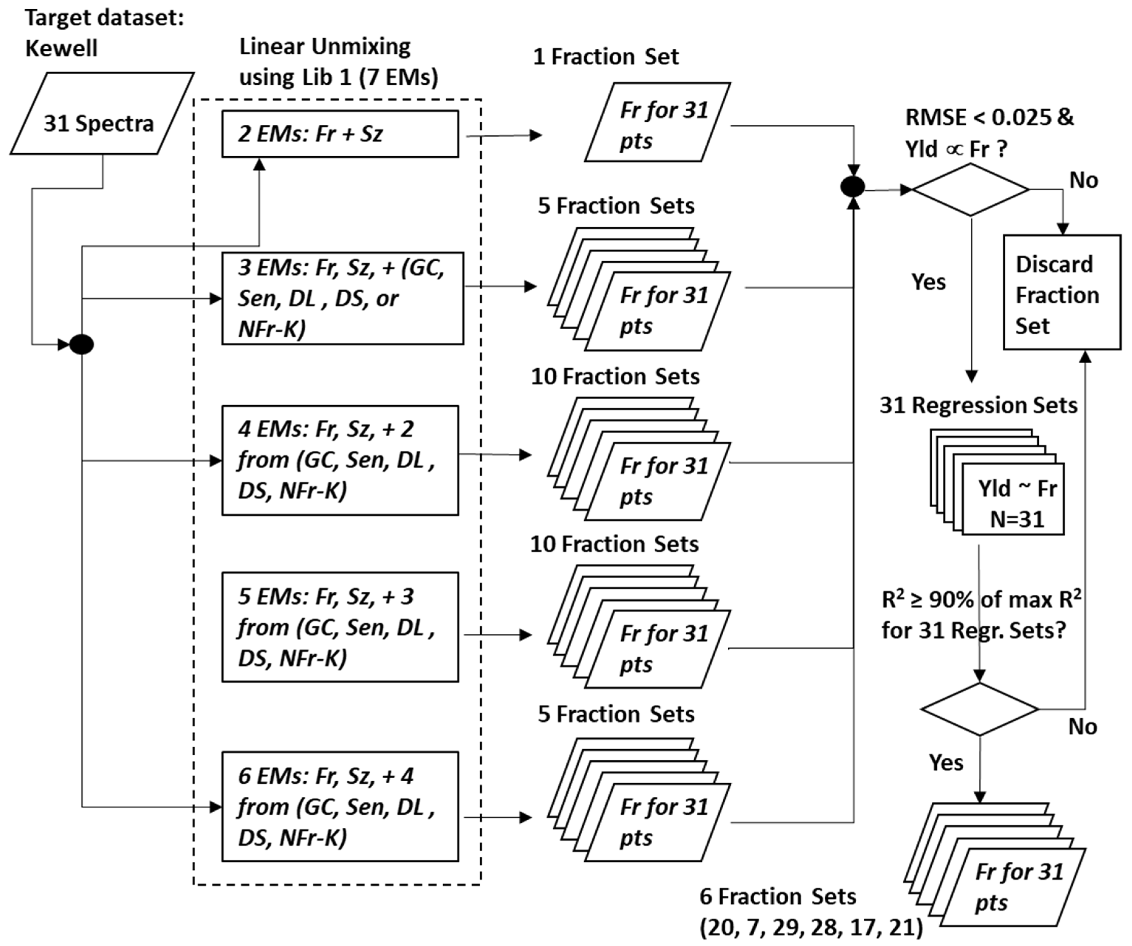
2.4. Spectral Mixture Analysis

The field spectra and EMs were imported as text data into ENVI (ver. 5.5, Harris Geospatial Solutions, Broomfield, CO USA) and saved as pseudo-images such that each “pixel” represented one spectrum. The SMA was run as a constrained model, summing to 1. The libraries that were assembled (Table 1) were used to unmix each of the five data sets using the linear spectral unmixing routine in ENVI. For each library, combinations of three to six fraction sets were run to unmix the data sets, resulting in 31 fraction sets (models) per library. Each fraction set (with an associated root-mean-square error (RMSE)) was saved as an ASCII file and imported into Excel for the selection of sets that met the criteria for the RMSE, fraction sum, and R² fit for yield.

SMA was used to quantify components within the mixed field spectra (pixels) based on the spectral libraries that contained “pure” spectra of the scene components [39] including frost and non-frost. That is, any given pixel can be described in terms of the proportion of the “pure” spectra for frost, and “pure” frosted/non-frosted spectra were used to explain the spectral variation within the three data sets. This was done by selecting reference spectra (EMs) from each data set to which mixed scene spectra were compared using a linear mixture model. A shade component was included to account for dark spectral components [40]. Note that the fraction component of interest (Fr, for example) can be corrected for shade: Fr_cor = Fr/(1 − Sz). This has been proposed as a method to improve the modelling of landscape features [39]; however, this did not improve any of the fits to yield in this study, and the Fr fractions presented are thus not shade corrected.

The RMSE was calculated as a measure of goodness of fit. A good fit of the measured (mixed) pixels to the resulting fraction model is determined by selecting a maximum threshold for the RSME, which, ideally, should be comparable to instrument noise [39]; in this case, it was set to values below 0.025 [38]. The combination of EMs in the selected model is then deemed a good description of the mixed pixel spectrum.

Fraction values that are greater than 1 or are negative are mathematically possible but they indicate EMs that do not represent the EM well or are not as “pure” as the ones in the measured mixed pixels [28]. The selection of EM sets that resulted in good fits of the fractions to the spectral data was determined by the RMSE data output from the mixture analysis and total fractions that summed to 1. To account for rounding errors, the fraction sum range was set at 0.999 to 1.001 and negative values for individual EM fractions were not excluded; this is discussed below.

The EM sets were also constrained to contain a Fr EM as the principal hypothesis was whether the Fr signature could be isolated from the mix of other EMs. Thus, the smallest EM set used for unmixing the target data sets required two EMs (Fr, Sz). The assessment of whether SMA models were able to quantify frost damage was determined by a linear regression using the coefficient of determination (R²) to measured yields at sampling locations across the data sets for the green (GL, GC), Fr, NFr, and Sen EMs. The final criterion for EM model selection was based on the direction of the slope for the R² regression fit to yield. It would be expected that as the Fr fraction increases (more frost damage), the impact on yield should be a negative relationship. If the slope of the relationship was positive, the fraction set was removed from subsequent analysis.

Initial unmixing was conducted with fraction sets without the Sz fraction to assess whether inclusion of this EM improved model fit. It was determined that the fraction sum (sum of all EMs in a set after unmixing) was equal to 1 only if a Sz EM was included in the EM set. Fraction sums that do not sum to unity indicate spectral components missing from the analysis such that the fitting algorithm cannot find a solution that fits the data well. Initial unmixing showed that EM sets that did not include the Sz EM always had lower R² values for the regression relationship of Fr fraction to yield when compared to similar sets with Sz (data not shown).

3. Results

3.1. Analysis Workflow

The analysis workflow is presented in Figure 2 using the Kewell data set as an example, but this applies to all five data sets. The target data set (Kewell) was unmixed for each spectral library, resulting in ten library outputs, one of which is shown for Kewell (Lib 1). From this output, all fraction sets that met the criteria (31) were derived, one for each combination of 2–6 EMs: 1 two-EM fraction set; 5 three-EM fraction sets; 10 four-EM fraction sets; 10 five-EM fraction sets; and 5 six-EM fraction sets. Each of these fraction sets contained a Fr fraction. Each set also contained an RMSE output (see above). If this was greater than 0.025 then the fraction set was removed from further analysis. After this, each Fr fraction was regressed against the yield for that data set (in this example, Kewell), and sets with a positive slope were excluded. The result was Fr fractions within each library and data set that could be used to assess which combination of EMs has the best regressions to yield.

In some analyses (e.g., the Kewell data set), all 31 fraction sets from a library met the selection criteria, while for others only a few or none met the criteria. The purpose of the analysis was not to assess all successful fraction sets but to select ones that had high R² to yield. Consequently, for each data set–library combination, the Fr fraction that had the highest R² to yield was selected as well as those in the top 10% of R² values (

Table 2. Summary of linear spectral mixture analysis of target data sets vs. endmember libraries for those libraries with the best-fitting Fr fraction to yield (within 10% of the highest R²) that met the selection criteria (see text). These top 10% fraction sets are listed in order of the R² value, from maximum to minimum. The mean RMSE, maximum R², and minimum R² of those top 10% fraction sets are listed. See Table 1 for the EMs contained in each library. See Table 3 for the EMs contained in each fraction set. Libraries with the best-fitting Fr fractions to yield (bolded) are presented in Figure 3.

Target Data Set	Library #	Library Name	Fraction RMSE Mean	Max R2	Min R2	Fraction Set #—Ranked by R2, Max to Min
Kewell	1	Kewell canopy	0.0051	0.75	0.69	20, 7, 29, 28, 17, 21
	2	PBC2006 canopy	0.0073	0.71	0.65	21, 29, 26, 31, 27, 23, 17, 28
	3	Kewell leaf	0.0063	0.64	0.57	10, 29, 21, 28, 17, 20, 31
	4	PBC2006 leaf	0.0071	0.70	0.58	27, 26, 31, 28, 23, 29, 13, 19
PBC2006	1	Kewell canopy	0.0063	0.63	0.57	8, 7, 20, 17, 10, 2, 21, 29
	2	PBC2006 canopy	0.0042	0.68	0.62	17, 28, 29, 27, 21, 7, 18, 30, 20, 31, 25, 26, 19, 8, 12, 23, 10, 13
	3	Kewell leaf	0.0151	0.57	0.52	2, 10
	4	PBC2006 leaf	0.0068	0.65	0.58	12, 25, 18, 23, 30, 7, 13, 20, 16, 22, 5, 10, 9, 28
	5	PBC2016′A’ head	0.0124	0.58	0.53	28, 9, 27, 18, 30, 22, 19
	6	PBC2016′A’ leaf	0.0168	0.57	0.52	2, 10
	7	PBC2016′A’ canopy	0.0074	0.58	0.53	9, 19, 13
	8	PBC2016′H’ canopy	0.0092	0.61	0.57	13, 5, 2
	9	PBC2016′H’ head	0.0108	0.61	0.56	19, 9, 2, 18, 28
	10	PBC2016′H’ leaf	0.0189	0.57	0.57	2
PBC2016	1	Kewell canopy	0.0126	0.41	0.41	8
	2	PBC2006 canopy	0.0133	0.36	0.36	13
	4	PBC2006 leaf	0.0127	0.38	0.36	19, 13
	6	PBC2016′A’ leaf	0.0241	0.31	0.31	8
	8	PBC2016′H’ canopy	0.0063	0.58	0.56	9, 19, 13, 8
	9	PBC2016′H’ head	0.0194	0.52	0.52	19
	10	PBC2016′H’ leaf	0.0219	0.35	0.35	8
PBC2016Heads	5	PBC2016′A’ head	0.0223	0.20	0.19	12, 16, 25
	9	PBC2016′H’ head	0.0098	0.18	0.17	25, 16, 12
PBC2016Leaves	6	PBC2016′A’ leaf	0.0175	0.11	0.09	25, 22, 12, 16, 20
	10	PBC2016′H’ leaf	0.0084	0.10	0.10	25

) to assess the similarity in Fr fraction regressions to yield. The 10% value was arbitrary (and another value could be chosen) but it allows comparison of the relatively best-fitting data sets to yield.

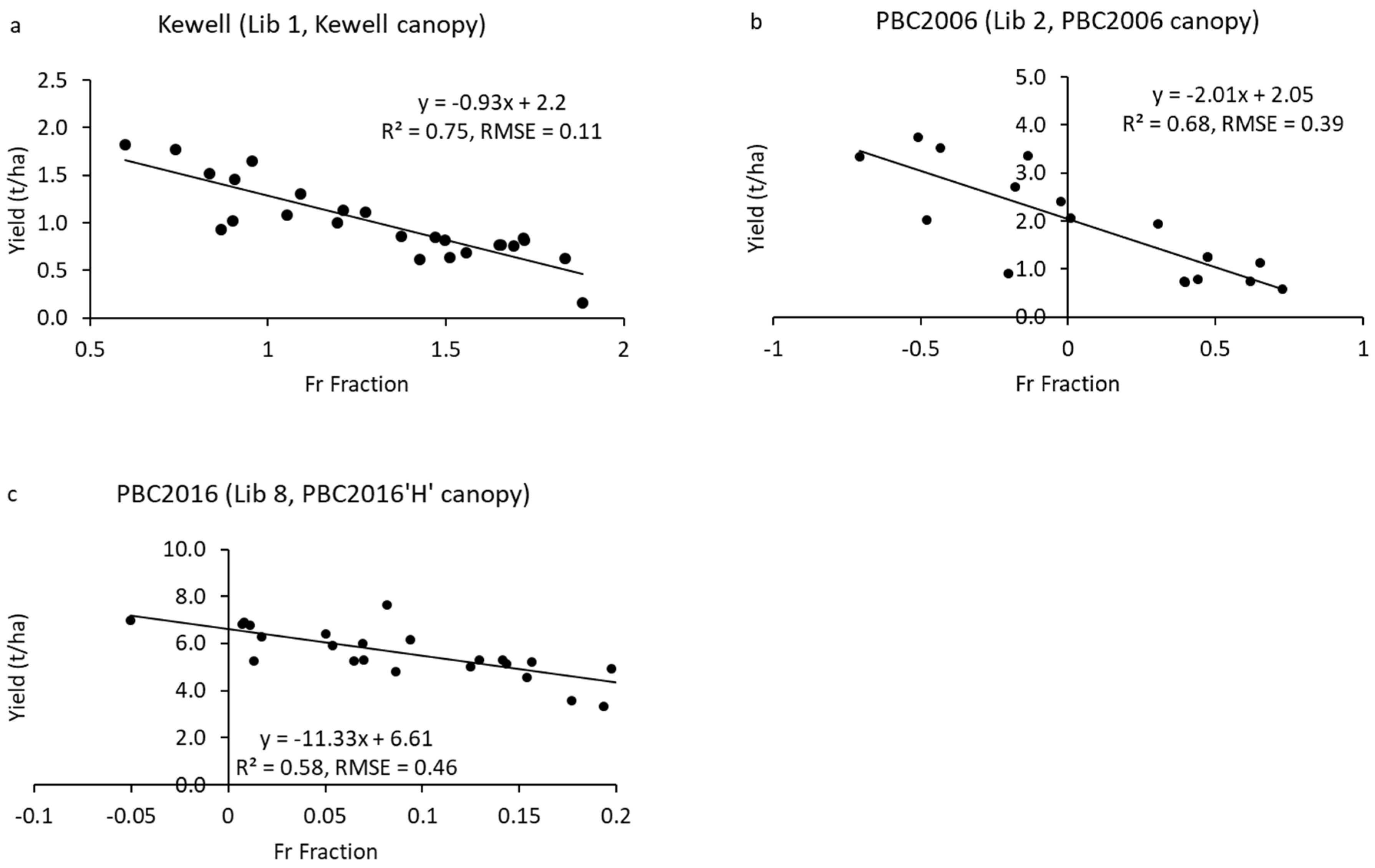
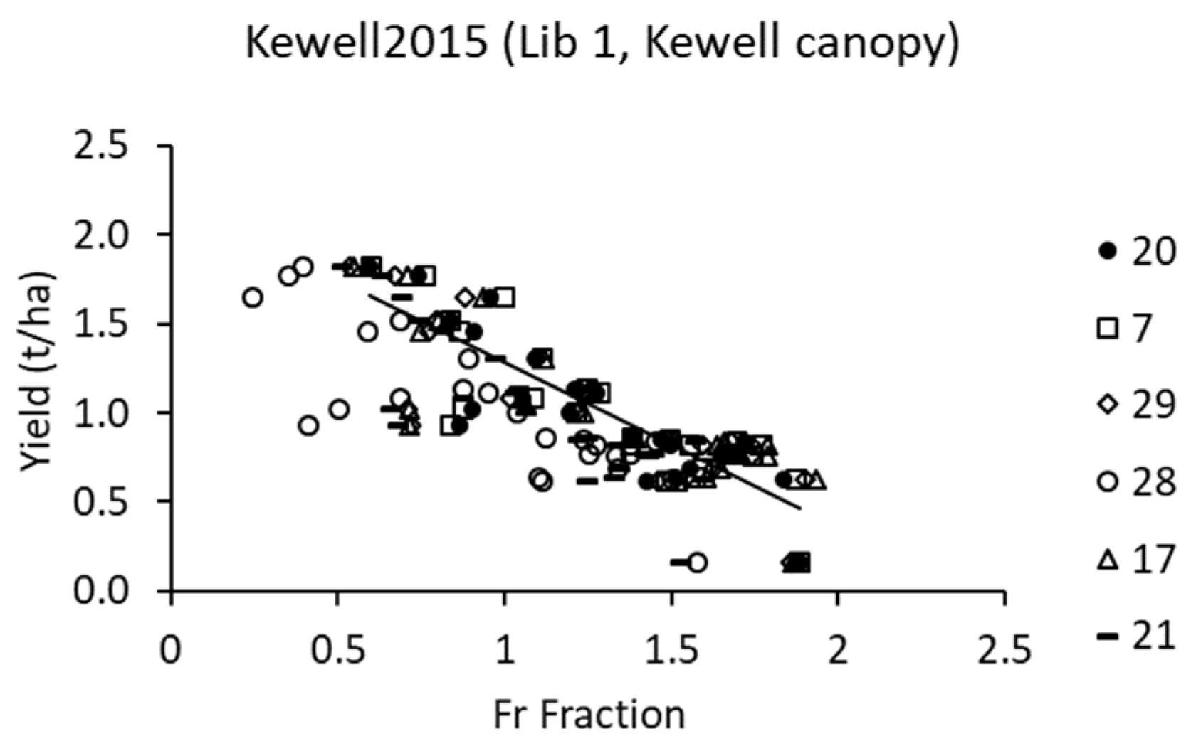
3.2. Deriving Fractions

For the Kewell data set, only Libraries 1, 2, 4, and 7 resulted in any fraction sets that fit the selection criteria (Table 2). For the PBC2006 data set, all the libraries (1–10) met the required criteria. The libraries that contained canopy-scale EMs showed the best fits to the data set (lowest RMSE). For the PBC2016 data set, the Kewell and PBC2006 libraries did not show good R² relationships to yield and neither did the PBC2016 (‘A’ or ‘H’) leaves. The PBC2016′H’ canopy and heads libraries showed Fr fractions with the best fits to the 2016 data set (R² = 0.58 and 0.52, respectively).

For example, the Fr signature from the Kewell data set showed the highest correlation to yield (R² = 0.75) for the “Kewell canopy” library when compared to other libraries used to unmix the data, such as the one containing PBC2006 (canopy) with a maximum R² = 0.71 for the best-fitting fraction set (Table 2). The PBC2006 data set maximum R² was 0.68 (in bold) and for PBC2016, it was 0.58, both with Fr fractions highest for the respective libraries with “canopy”-scale EMs. These also showed the lowest fraction RMSE, indicating the best model fits from the SMA. The respective libraries with “green leaf” EMs also showed low RMSE fits (for the Kewell and PBC2006 data sets) but did not necessarily result in the highest R² values to yield for the Fr fraction, although the PBC2006 was second after the “canopy” EM R² fit. It was similar for the “head” data sets: they met the criteria for unmixing but were not as good as those libraries containing a “canopy” EM. The RMSE values listed in Table 2 are means for the top 10% of fraction sets listed, representing the general mixture model fit of the best fraction sets listed.

The PBC2016 heads and leaves data sets were only fit with libraries with EMs derived from head- and leaf-scale measurements. Although there were fraction sets with Fr fractions that were less than the 0.025 criterion, the R² fits to yield were very low (e.g., data set PBC2016Leaves, Lib 10, RMSE = 0.0084, R² = 0.10).

The best-fitting Fr fraction from each data set (Table 2, in bold) was plotted (Figure 3) to show the relationships to yield, and the RMSE for yield ranged from 0.11 to 0.46 t ha⁻¹. As the Fr fraction increased, the yield decreased. Each of these was selected from a different fraction set resulting from the unmixing of each library. Although there were clear relationships between Fr fractions and yield, the fraction sets from which each Fr fraction originated differed across data sets. If fractions are to be used more universally, the same fraction sets need to be selected across the data sets.

Although there was no single “universal” fraction set that was the best fit across all data sets, the Fr fractions within a given fraction set showed similar fitting parameters to yield. For example, the Kewell data set showed that all the Fr fractions from the top 10% of R² fits to yield (Table 2) fell within a similar data space (Figure 4). The linear parameters (slope, R², and range) are similar, suggesting that the Fr fraction from any of the fraction sets that met the basic selection criteria could be used to estimate yield response and that selecting just the fraction set with the maximum R² fit was not necessary to determine a fraction that fit well to yield. The other data sets showed similar patterns. Thus, the specifics of the Fr fraction linear parameters change but the basic relationships to yield are similar across mixing models.

To discover if there was a library containing a fraction set that has a good R² to yield across the data sets, the top 10% models (Table 2) were compared to determine if there were fraction sets in common across the data sets for the Fr EMs (

Table 3. List of fraction sets and EMs within each set. The top 10% best-fitting models for yield (from Table 2) are listed for these libraries and data sets: K = Kewell data set, Library 1 (Kewell canopy), P06 = PBC2006 data set, Library 2 (PBC2006 canopy), P16 = PBC2016 data set, Library 8 (PBC2016′H’ canopy). Asterisks mark the fraction sets with the best R² fit (i.e., 9, 17, 20) for the particular library (P16, P06, K) to yield (in bold Table 2) and displayed in Figure 3.

Fraction Set Number	EM1	EM2	EM3	EM4	EM5	EM6	Best Fit to Yield
1	Fr	Sz
2	GC/GL	Fr	Sz
3	SDL	Fr	Sz
4	DS	Fr	Sz
5	NFr	Fr	Sz
6	Sen	Fr	Sz
7	GC/GL	DL	Fr	Sz			K, P06
8	GC/GL	DS	Fr	Sz			P06, P16
9	GC/GL	NFr	Fr	Sz			P16*
10	GC/GL	Sen	Fr	Sz			P06
11	DL	DS	Fr	Sz
12	DL	NFr	Fr	Sz			P06
13	DS	NFr	Fr	Sz			P06, P16
14	Sen	DL	Fr	Sz
15	Sen	DS	Fr	Sz
16	Sen	NFr	Fr	Sz
17	GC/GL	DL	DS	Fr	Sz		K, P06*
18	GC/GL	DL	NFr	Fr	Sz		P06
19	GC/GL	DS	NFr	Fr	Sz		P06, P16
20	GC/GL	Sen	DL	Fr	Sz		K*, P06
21	GC/GL	Sen	DS	Fr	Sz		K, P06
22	GC/GL	Sen	NFr	Fr	Sz
23	DL	DS	NFr	Fr	Sz		P06
24	Sen	DL	DS	Fr	Sz
25	Sen	DL	NFr	Fr	Sz		P06
26	Sen	DS	NFr	Fr	Sz		P06
27	GC/GL	Sen	DS	NFr	Fr	Sz	P06
28	GC/GL	DL	DS	NFr	Fr	Sz	K, P06
29	GC/GL	Sen	SDL	DS	Fr	Sz	K, P06
30	GC/GL	Sen	SDL	NFr	Fr	Sz	P06
31	Sen	SDL	DS	NFr	Fr	Sz	P06

). As noted in Table 2, the 2016PBCHeads and 2016PBCLeaves data sets could not be fit with any of the libraries for the Fr fraction, leaving only three data sets to test. Although none of the fraction sets had all three data sets in common, the comparison between the PBC2006 and PBC2016 data sets showed several commonalities, with fraction sets 8, 13, and 19 (Table 2) showing high R² to yield across the site-years. The distinctive feature in these was the inclusion of the dry soil (DS) EM. This spectral signature was acquired at the PBC site, and both these studies were performed at this location on the same soil type. The fraction sets (for Fr EM) in common for the Kewell (K) and PBC2016 data sets (P16) for yield were 7, 17, 20, 21, 28, and 29. This tended to include the dead leaf (DL) or senescent (Sen) EMs but was also mixed with the dry soil (DS). With one exception (K for fraction set 2, Kewell) the best-fitting fraction sets contained 4–6 EMs.

3.3. Multiple Endmember Spectral Mixture Modelling (MESMA)

The multiple endmember spectral mixture modelling (MESMA) approach to allowing EMs to vary for each pixel [38] was tested on the Kewell data using the VIPER plug-in to the ENVI software. The results did not show any improvement of fit to yield, and there were pixels (data points in the pseudo-image) that were not selected because they did not meet all the selection criteria, resulting in few data points for analysis. The MESMA approach is appropriate for larger data sets (such as imagery) and with large libraries for inclusion of a wide range of spectral variability.

3.4. Comparison to NDVI

It is important to know whether there might be a simpler method for mapping frost damage across agricultural fields. The normalized difference vegetation index (NDVI, [41]) is ubiquitous in the agricultural remote sensing community, and it would be tempting to use this index to map frost within a short period after a known frost event. The NDVI was calculated from the spectral data by calculating the mean for the red (670–680 nm) and NIR (850–860 nm) portion of the spectrum for each of the data sets (

Table 4. Coefficient of determination (R²) between normalized difference vegetation index (NDVI) values and yield for the five data sets.

Data Set.	Yield R2
PBC2006	0.55
Kewell	0.03
PBC2016	0.34
PBC2016Heads	0.06
PBC2016Leaves	0.08

). The only data set that showed a moderate response (R² = 0.55) was the PBC2006 data.

4. Discussion

Although yield can be impacted by a range of biophysical factors, such as drought, infestation of pests and weeds, soil type, and landscape position, our results show that, despite these potentially confounding factors, frost fractions derived from SMA can be used to detect frost damage in wheat. While frost fractions were able to estimate yield at the canopy scale, there was no “universal” EM set from which a frost fraction could be derived. All but one of the fraction sets that exhibited “best fit” had a green EM along with the Fr and Sz. Otherwise, a mix of EMs was required for prediction as no unique set of EMs was found to unmix all data sets.

The main factors of green, senescent, dead, frost-affected, soil, and shade are not possible to measure simultaneously. Thus, though it was recognized that there is variation in canopies, particularly across time [42], it was proposed that a simple collection of standardized or “fixed” EMs from a library representing important canopy components might suffice for segregating specific spectral components from a mixed hyperspectral signal [38]. This approach allowed for the isolation of a frost signal or component in the data, confirming that it is feasible that with a set of fixed EMs derived from similar crops (earlier in the season before frost has occurred) or from a reference area within a field (with relatively less frost damage), frost-damaged areas can be isolated. Despite the inability to identify a “universal” set of EMs to unmix spectra across these data sets, it is possible that with data from more sites and further analysis, a generic set of EMs for frost mapping might be established.

The results show promise for unmixing canopy-scale spectra. None of the libraries containing canopy-scale spectra were successful in unmixing the head and leaf data, which is not surprising since heads and leaves would not be expected to contain the complexity of a canopy (including shade, for example). The libraries with head- and leaf-scale EMs were able to unmix the canopy-scale data but the model fits and relationships to yield were not as strong as for those libraries with canopy-scale green EMs, indicating some scale dependencies in application of the EMs to mixed spectra. The importance of collecting measurements at the appropriate scale was identified previously [27,43], but it has not been clear for SMA whether this was an important consideration. The improvement in both model fits (lower RMSE) and relationships to yield (R²) within the canopy-scale EMs could be due to the inclusion of nonlinear mixing effects of light within canopies [29], but this is an issue that is still unresolved. There were acceptable model fits for Fr fractions derived from libraries containing EMs of head and leaf spectra to unmix data sets of head and leaf, but the ability to estimate yield was extremely low. Thus, component-scale EMs (heads and leaves) can be used in canopy mixture models with other EMs to quantify frost damage, but assessing frost damage using the Fr fraction at the plant component scale does not result in good estimates of canopy-scale frost damage. Finally, the best estimate of frost damage used the green canopy-scale EM.

The unmixing process identified fraction sets with 4–6 EMs as the best fitting. This presumably was because the canopies were sufficiently complex and could not be modelled with fewer EMs [44]. In mixture analysis, one criterion for selection is the fraction set with the fewest EMs [38], in which case a four-EM set would be preferred. However, because a set of “fixed” EMs was used, this was not as important a criterion since, effectively, only the NFr and Fr EMs varied across the data sets. Thus, the question about model fit using the RMSE and ability to estimate frost damage was more relevant.

In mixture modelling, the constrained model where the fraction sums are between 0 and 1 is also a selection criterion for good modeling of the data. Negative values are mathematically feasible if the EMs selected are not as “pure” a representation of the scene’s components as those in the target scene or data set as a whole [28]. Because it was expected that the spectral signature (EM) of frost might vary and is not a fixed element in the scene, varying with degree of damage, time after frost event, other environmental conditions, and genetics, EM fractions that were negative or greater than unity were included in the analysis. Knowing the absolute fraction was not as important as the relationship to yield.

The NDVI is a ubiquitous index used to measure many plant and canopy parameters and is most suited to measuring biophysical factors at the canopy scale [31]. Although many others could have been reported, this was chosen as the most likely to be used for the remote sensing of abiotic stress and compared for discussion against the full spectral analysis presented here. Its ability to measure frost damage was compared to the spectral unmixing procedure since it is simple to implement. If the relationship between NDVI and yield, as a correlate of frost impact, was straightforward, it would be a clear choice for frost damage mapping. However, it was found that the NDVI was unable to estimate frost damage to yield when compared with the Fr fraction. This is not unexpected as NDVI measures canopy cover [45].

Further research is needed with a broader range of data from natural field conditions to continue development of the unmixing concept for frost damage assessment. In particular, is there a representative frost signature that could be developed, or a small set of signatures based on a set of conditions determined by crop or field type (e.g., crop variety, days after frost, etc.) that could be useful? The use of multispectral data would simplify the use of remote sensing tools. Thus, a larger data set collected from fields with known frost conditions would allow for the selection of a minimum set of targeted wavebands, potentially leading to simpler instruments for frost assessment for use in unmanned aerial vehicles, aircraft, or satellites. The question of waveband width would also serve to inform the spectral resolution needed for a multispectral system. Waveband position, width, and number required could be assessed by de-convolving the hyperspectral data collected in this study combined with a broader data set, and this would be the next step in research. Importantly, validation experiments to test the ability to predict areas where frost has occurred and map the damage are needed to develop tools for growers to make informed decisions for cutting hay, altering grain marketing strategies, and harvest planning.

5. Conclusions

We showed that it was possible to develop good relationships between frost fractions derived from mixture analysis of hyperspectral data and yield. There were, however, some complexities in terms of being able to derive unique fraction relationships to yield for use across different data sets. It was determined that assessing frost damage at the component scale (e.g., leaf or head) does not result in good estimates of canopy-scale frost damage. Further, the best results for quantifying frost damage were attained with libraries containing canopy-scale spectra. This research highlighted that there is opportunity to move beyond the traditional use of NDVI for the identification of generic stresses to a targeted approach for mapping an abiotic stress. Future work requires more natural frost data from fields to build larger data sets and spectral libraries. Identifying signatures that could uniquely and more universally identify frost is needed if this is to be useful for the autonomous mapping of frost. This will also require field validation of the frost assessment techniques. Identification of a subset of wavebands and widths might allow for the development of simpler sensors or imagers for frost detection. Finally, the power of using hyperspectral data will likely be realized when signatures for multiple stresses are developed for the simultaneous mapping of biotic and abiotic factors that affect crop production.

References

1. Duddu, H.S.N.; Pajic, V.; Noble, S.D.; Tanino, K.K.; Shirtliffe, S.J. Image-Based Rapid Estimation of Frost Damage in Canola (Brassica napus L.). Can. J. Remote Sens. 2018, 44, 169–175. [Google Scholar] [CrossRef]
2. Maqbool, A.; Shafiq, S.; Lake, L. Radiant frost tolerance in pulse crops—A review. Euphytica 2010, 172, 1–12. [Google Scholar] [CrossRef]
3. Martino, D.L.; Abbate, P.E. Frost damage on grain number in wheat at different spike developmental stages and its modelling. Eur. J. Agron. 2019, 103, 13–23. [Google Scholar] [CrossRef]
4. Boer, R.; Campbell, L.; Fletcher, D. Characteristics of frost in a major wheat-growing region of Australia. Aust. J. Agric. Res. 1993, 44, 1731–1743. [Google Scholar] [CrossRef] [Green Version]
5. Mushtaq, S.; An-Vo, D.-A.; Christopher, M.; Zheng, B.; Chenu, K.; Chapman, S.C.; Christopher, J.T.; Stone, R.C.; Frederiks, T.M.; Alam, G.M.M. Economic assessment of wheat breeding options for potential improved levels of post head-emergence frost tolerance. Field Crops Res. 2017, 213, 75–88. [Google Scholar] [CrossRef]
6. Paulsen, G.M.; Heyne, E.G. Grain Production of Winter Wheat after Spring Freeze Injury1. Agron. J. 1983, 75, 705–707. [Google Scholar] [CrossRef]
7. March, T.; Knights, S.; Biddulph, B.; Ogbonnaya, F.; Maccallum, R.; Belford, R.K. The GRDC National Frost Initiative. In Proceedings of the GRDC Updates, Adelaide, Australia, 10 February 2015. [Google Scholar]
8. Marcellos, H.; Single, W. Temperatures in wheat during radiation frost. Aust. J. Exp. Agric. 1975, 15, 818–822. [Google Scholar] [CrossRef]
9. The Intergovernmental Panel on Climate Change; Field, C.B.; Barros, V.; Stocker, T.F.; Dahe, Q. Managing the Risks of Extreme Events and Disasters to Advance Climate Change Adaptation: Special Report of the Intergovernmental Panel on Climate Change; Cambridge University Press: Cambridge, UK, 2012. [Google Scholar]
10. Fuller, M.P.; Fuller, A.M.; Kaniouras, S.; Christophers, J.; Fredericks, T. The freezing characteristics of wheat at ear emergence. Eur. J. Agron. 2007, 26, 435–441. [Google Scholar] [CrossRef]
11. Porter, J.; Gawith, M. Temperatures and the growth and development of wheat: A review. Eur. J. Agron. 1999, 10, 23–36. [Google Scholar] [CrossRef]
12. Cromey, M.G.; Wright, D.S.C.; Boddington, H.J. Effects of frost during grain filling on wheat yield and grain structure. N. Z. J. Crop Hortic. Sci. 1998, 26, 279–290. [Google Scholar] [CrossRef]
13. Al-Issawi, M.; Rihan, H.Z.; El-Sarkassy, N.; Fuller, M.P. Frost Hardiness Expression and Characterisation in Wheat at Ear Emergence. J. Agron. Crop Sci. 2013, 199, 66–74. [Google Scholar] [CrossRef]
14. Marcellos, H.; Single, W. Frost Injury in Wheat Ears After Ear Emergence. Funct. Plant Biol. 1984, 11, 7–15. [Google Scholar] [CrossRef]
15. Frederiks, T.M.; Christopher, J.T.; Sutherland, M.W.; Borrell, A.K. Post-head-emergence frost in wheat and barley: Defining the problem, assessing the damage, and identifying resistance. J. Exp. Bot. 2015, 66, 3487–3498. [Google Scholar] [CrossRef] [PubMed]
16. Macedo-Cruz, A.; Pajares, G.; Santos, M.; Villegas-Romero, I. Digital Image Sensor-Based Assessment of the Status of Oat (Avena sativa L.) Crops after Frost Damage. Sensors 2011, 11, 6015–6036. [Google Scholar] [CrossRef]
17. Flower, K.; Boruss, B.; Nansen, C.; Jones, H.; Thompson, S.; Lacoste, C.; Murphy, M. Proof of Concept: Remote Sensing Frosted-Induced Stress in Wheat Paddocks; Grains Research and Development Corporation: Canberra, Australia, 2014; p. 36. [Google Scholar]
18. Wu, Q.; Zhu, D.; Wang, C.; Ma, Z.; Wang, J. Diagnosis of freezing stress in wheat seedlings using hyperspectral imaging. Biosyst. Eng. 2012, 112, 253–260. [Google Scholar] [CrossRef]
19. Nuttall, J.G.; Perry, E.M.; Delahunty, A.J.; O’Leary, G.J.; Barlow, K.M.; Wallace, A.J. Frost response in wheat and early detection using proximal sensors. J. Agron. Crop Sci. 2019, 205, 220–234. [Google Scholar] [CrossRef]
20. Perry, E.M.; Nuttall, J.G.; Wallace, A.J.; Fitzgerald, G.J. In-field methods for rapid detection of frost damage in Australian dryland wheat during the reproductive and grain-filling phase. Crop Pasture Sci. 2017, 68, 516–526. [Google Scholar] [CrossRef]
21. Stutsel, B. Temperature Dynamics in Wheat (Triticum Aestivum) Canopies during Frost; The University of Western Australia: Perth, Australia, 2019. [Google Scholar]
22. Rebbeck, M.; Knell, G.; Hayman, P.; Lynch, C.; Alexander, B.; Faulkner, M.; Gusta, L.; Duffield, T.; Curtin, S.; Falconer, D. Managing Frost Risk: A Guide for Southern Australian Grains; South Australian Research and Development Institure and Grains Research and Development Corporation: Canberra, Australia, 2007; p. 64. [Google Scholar]
23. Feng, W.; Yao, X.; Zhu, Y.; Tian, Y.C.; Cao, W.X. Monitoring leaf nitrogen status with hyperspectral reflectance in wheat. Eur. J. Agron. 2008, 28, 394–404. [Google Scholar] [CrossRef]
24. Bock, C.H.; Poole, G.H.; Parker, P.E.; Gottwald, T.R. Plant Disease Severity Estimated Visually, by Digital Photography and Image Analysis, and by Hyperspectral Imaging. Crit. Rev. Plant Sci. 2010, 29, 59–107. [Google Scholar] [CrossRef]
25. Fitzgerald, G.J.; Maas, S.J.; Detar, W.R. Spider Mite Detection and Canopy Component Mapping in Cotton Using Hyperspectral Imagery and Spectral Mixture Analysis. Precis. Agric. 2004, 5, 275–289. [Google Scholar] [CrossRef]
26. Masoni, A.; Ercoli, L.; Mariotti, M. Spectral Properties of Leaves Deficient in Iron, Sulfur, Magnesium, and Manganese. Agron. J. 1996, 88, 937–943. [Google Scholar] [CrossRef]
27. Cotrozzi, L.; Townsend, P.A.; Pellegrini, E.; Nali, C.; Couture, J.J. Reflectance spectroscopy: A novel approach to better understand and monitor the impact of air pollution on Mediterranean plants. Environ. Sci. Pollut. Res. 2018, 25, 8249–8267. [Google Scholar] [CrossRef]
28. Adams, J.B.; Gillespie, A.R. Remote Sensing of Landscapes with Spectral Images: A Physical Modeling Approach; Cambridge University Press: Cambridge, UK, 2006. [Google Scholar] [CrossRef]
29. Somers, B.; Asner, G.P.; Tits, L.; Coppin, P. Endmember variability in Spectral Mixture Analysis: A review. Remote Sens. Environ. 2011, 115, 1603–1616. [Google Scholar] [CrossRef]
30. Nakagawa, S.; Santos, E.S.A. Methodological issues and advances in biological meta-analysis. Evol. Ecol. 2012, 26, 1253–1274. [Google Scholar] [CrossRef]
31. Fitzgerald, G.; Rodriguez, D.; O’Leary, G. Measuring and predicting canopy nitrogen nutrition in wheat using a spectral index—The canopy chlorophyll content index (CCCI). Field Crops Res. 2010, 116, 318–324. [Google Scholar] [CrossRef]
32. March, T.; Laws, M.; Eckermann, P.; Reinheimer, J.; Biddulph, B.; Eglinton, J. Frost Tolerance: Identifying Robust Varieties; Grains Research Development Corporation: Adelaide, Australia, 2013. [Google Scholar]
33. Reinheimer, J.L.; Barr, A.R.; Eglinton, J.K. QTL mapping of chromosomal regions conferring reproductive frost tolerance in barley (Hordeum vulgare L.). Theor. Appl. Genet. 2004, 109, 1267–1274. [Google Scholar] [CrossRef]
34. Zadoks, J.C.; Chang, T.T.; Konzak, C.F. A decimal code for the growth stages of cereals. Weed Res. 1974, 14, 415–421. [Google Scholar] [CrossRef]
35. Biddulph, B.; Laws, M.; Eckermann, P.; Maccallam, R.; Leske, B.; March, T.; Eglinton, J. Preliminary ratings of wheat varieties for susceptibility to reproductive frost damage. In Proceedings of the GRDC Updates, Murray Bridge, Australia, 12 February 2015. [Google Scholar]
36. White, C. Cereals—Frost Identification The Back Pocket Guide. In Bulletin 4375; Grains Research and Development Corporation: Canberra, Australia; Government of Western Australia Dept. of Agriculture: Kensington, Australia, 2000; p. 12. [Google Scholar]
37. Stutsel, B.M.; Callow, J.N.; Flower, K.; Biddulph, T.B.; Cohen, B.; Leske, B. An Automated Plot Heater for Field Frost Research in Cereals. Agronomy 2019, 9, 96. [Google Scholar] [CrossRef]
38. Roberts, D.A.; Gardner, M.; Church, R.; Ustin, S.; Scheer, G.; Green, R.O. Mapping Chaparral in the Santa Monica Mountains Using Multiple Endmember Spectral Mixture Models. Remote Sens. Environ. 1998, 65, 267–279. [Google Scholar] [CrossRef]
39. Smith, M.O.; Ustin, S.L.; Adams, J.B.; Gillespie, A.R. Vegetation in deserts: I. A regional measure of abundance from multispectral images. Remote Sens. Environ. 1990, 31, 1–26. [Google Scholar] [CrossRef]
40. Adams, J.B.; Smith, M.O.; Johnson, P.E. Spectral mixture modeling: A new analysis of rock and soil types at the Viking Lander 1 Site. J. Geophys. Res. Solid Earth 1986, 91, 8098–8112. [Google Scholar] [CrossRef]
41. Rouse, J.W., Jr.; Haas, R.H.; Schell, J.A.; Deering, D.W. Monitoring vegetation systems in the Great Plains with ETRS. In Proceedings of the Third Earth Resources Technology Satellite-1 Symposium, Goddard Space Flight Cent., Washington, DC, USA, 10–14 December 1973; pp. 309–317. [Google Scholar]
42. Bateson, C.A.; Asner, G.P.; Wessman, C.A. Endmember bundles: A new approach to incorporating endmember variability into spectral mixture analysis. IEEE Trans. Geosci. Remote Sens. 2000, 38, 1083–1094. [Google Scholar] [CrossRef]
43. Cammarano, D.; Fitzgerald, G.J.; Casa, R.; Basso, B. Assessing the Robustness of Vegetation Indices to Estimate Wheat N in Mediterranean Environments. Remote Sens. 2014, 6, 2827–2844. [Google Scholar] [CrossRef] [Green Version]
44. Fitzgerald, G.J.; Pinter, P.J.; Hunsaker, D.J.; Clarke, T.R. Multiple shadow fractions in spectral mixture analysis of a cotton canopy. Remote Sens. Environ. 2005, 97, 526–539. [Google Scholar] [CrossRef]
45. Fitzgerald, G.J. Characterizing vegetation indices derived from active and passive sensors. Int. J. Remote Sens. 2010, 31, 4335–4348. [Google Scholar] [CrossRef]
Figure 1. (a) Fixed EMs used in all libraries. GC = green canopy, GL = green leaf, DL = dead leaf, DS = dry soil, Sen = senescent leaf, Sz = shade (zero). Derived from the PBC2006 data set. See the text for descriptions. (b) Frost and non-frost EMs for field sites. NFr-Kewell, Fr-Kewell = non-frost and frost at Kewell; NFr-PBC2006, Fr-PBC2006 = non-frost and frost, Plant Breeding Center 2006. (c) Non-frost (control) EMs for the 2016 Plant Breeding Center experiment. NFr = non-frosted, 20161103 and 20161111 = measurement dates, C = wheat canopy, H = wheat heads, L = wheat leaves. (d) Frost EMs for the 2016 Plant Breeding Center experiment. Fr = frost, 20161103′H’ = measurement date, ‘H’ = measurements collected on heading experiment. C = wheat canopy, H = wheat heads, L = wheat leaves. (e) Frost EMs for the 2016 Plant Breeding Center experiment. Fr = frost, 20161103′A’ and 20161111′A’ = measurement dates, ‘A’ = measurements collected on anthesis experiment. C = wheat canopy, H = wheat heads, L = wheat leaves. For all data sets, leaf and head data were collected using a spectrometer leaf clamp.
Remotesensing 11 02476 g001
Figure 2. Workflow for comparison of the 10 spectral libraries across the five target data sets. This figure uses the analysis of the Kewell canopy library (Lib 1) for linear unmixing of the Kewell target data set as one example. The spectral unmixing for each combination of spectral libraries and target data set was performed using two, three, four, five, and six EMs, resulting in 31 fraction sets. After checking that the root-mean-square error (RMSE) met the 0.025 threshold, and that yield was negatively correlated with Fr, all 31 fraction sets for the Kewell data set were used for regression analysis relative to yield. Fraction sets that were within 10% of the highest R2 to yield (6 of 31 in this case) continued to final analysis.
Remotesensing 11 02476 g002
Figure 3. Best-fitting Fr fractions for each of the three data sets for yield for fraction sets (Table 2): (a) 20, (b) 17, (c) 9. See Table 3 for fraction set compositions.
Remotesensing 11 02476 g003
Figure 4. Fr fractions from fraction sets: Kewell data set, Library 1 (Kewell canopy) (Table 2). The legend numbers are the individual fraction sets representing the source of the Fr fraction that fit the yield best (top 10%) as described in Table 2. The line fit is the same as that in Figure 3a. Individual EMs in each fraction set are listed in Table 3.
Remotesensing 11 02476 g004