Combining Measurements of Built-up Area, Nighttime Light, and Travel Time Distance for Detecting Changes in Urban Boundaries: Introducing the BUNTUS Algorithm


Abstract
:
1. Introduction
- R1
- The study is global, so we may only choose globally consistent and available datasets.
- R2
- We wish to study enough cities to establish patterns, so the algorithm must be computationally efficient enough for large-scale use.
- R3
- Changes in urban extent can be small, so the algorithm must work at high resolution, no more than 1 km.
- R4
- The study must be long enough to establish trends. We estimate this requires two decades of data.
2. Review of Existing Methods
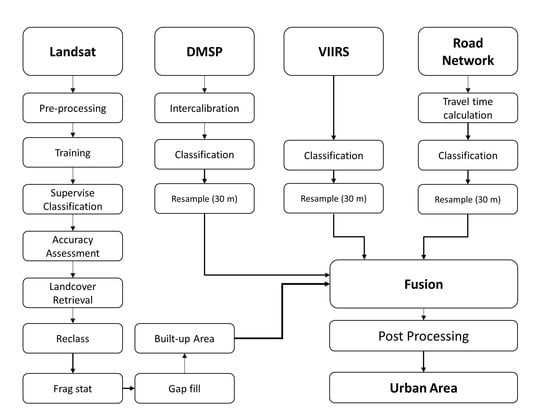
3. Methodology
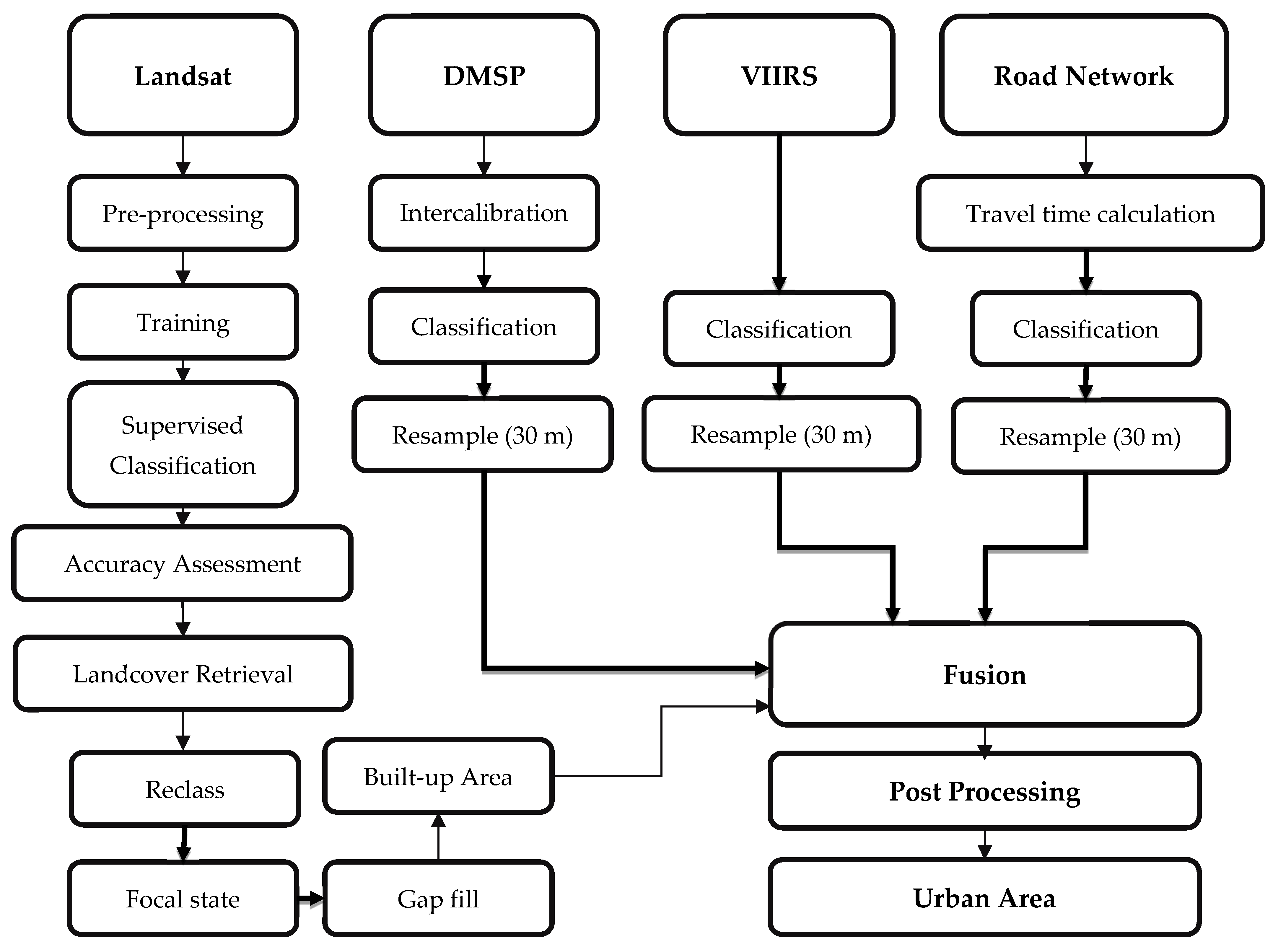
3.1. Case Studies
3.2. Land Cover Classification
- Dealing with the inevitable instabilities arising from different instruments and conditions;
- A lack of trustworthy and independent data points for training the classification;
- The computational demands of classification at this resolution.
3.2.1. Accuracy Assessment
3.2.2. Urban Area Generation
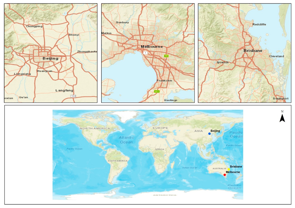
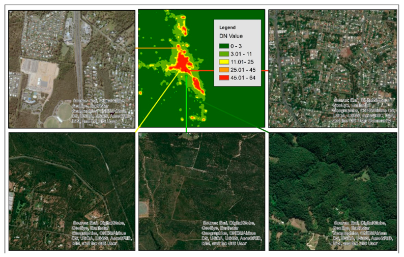
3.3. Nighttime Light Data Processing
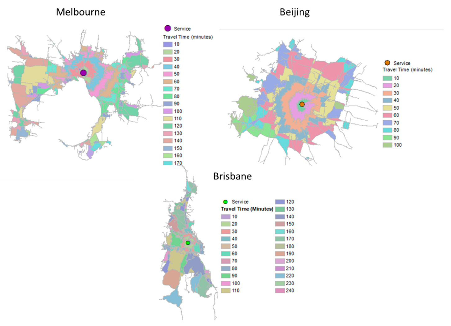
3.4. Travel Distance Raster Creation
3.5. Fusion of Datasets
3.6. Processing Time and Equipment
4. Results
4.1. Validating BUNTUS
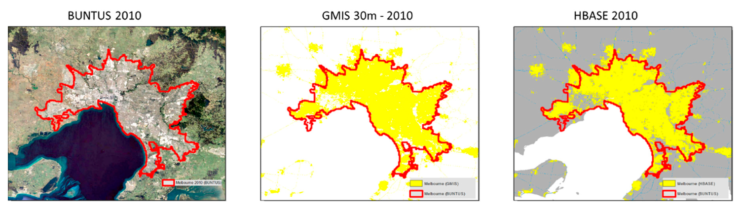
4.2. Comparison
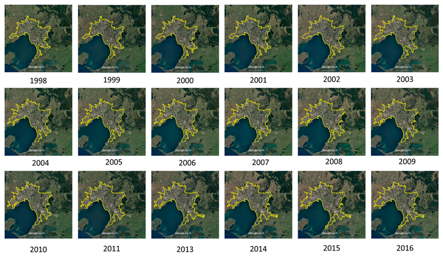
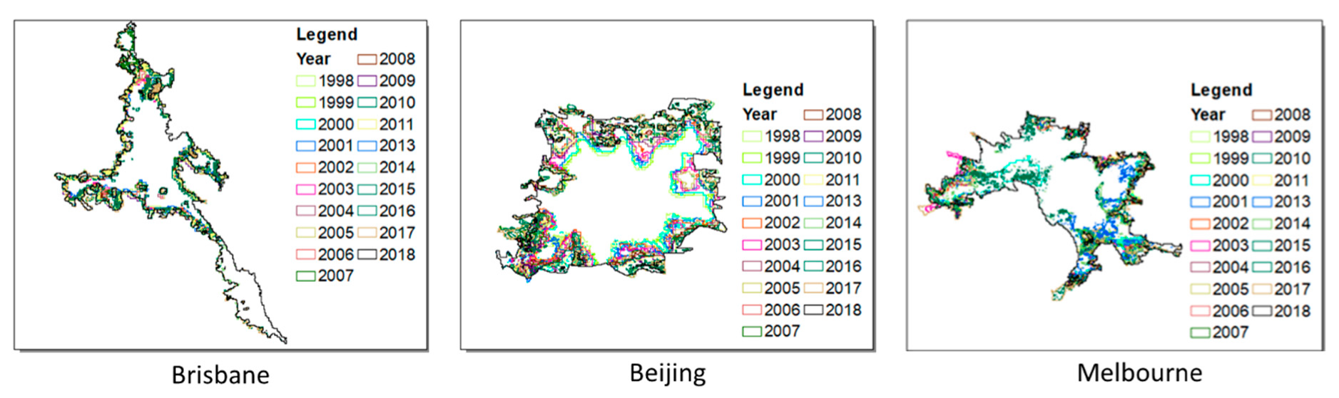
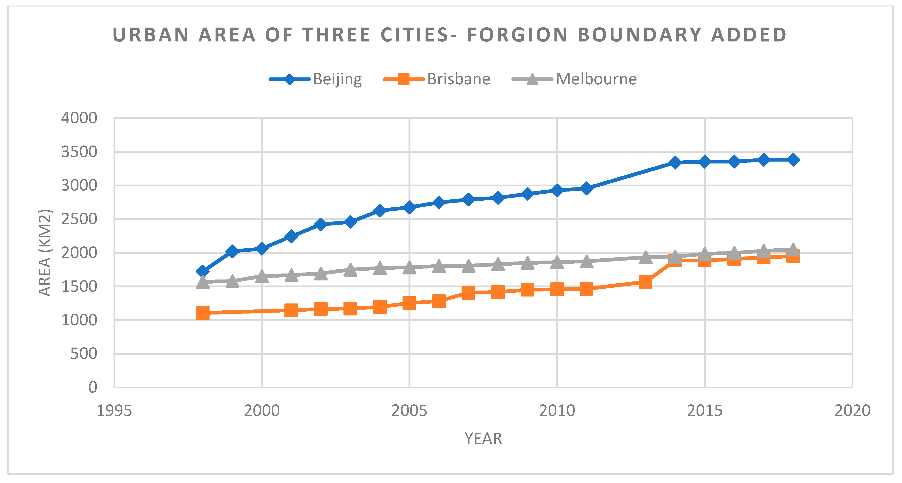
4.3. Urban Expansion
5. Discussion and Limitations
5.1. Discussion
5.2. Limitations
6. Conclusions
7. Future Work
Author Contributions
Funding
Acknowledgments
Conflicts of Interest
References
- United Nations. World Urbanization Prospects 2018—Population Division—United Nations. 2018. Available online: https://esa.un.org/unpd/wup/ (accessed on 13 June 2018).
- Hoornweg, D.; Sugar, L.; Trejos Gómez, C.L. Cities and Climate Change: An Urgent Agenda; World Bank: Washington, DC, USA, 2010. [Google Scholar]
- Bettencourt, L.; West, G. A unified theory of urban living. Nature 2010, 467, 912–913. [Google Scholar] [CrossRef] [PubMed]
- Brown, M.A.; Southworth, F.; Sarzynski, A. The geography of metropolitan carbon footprints. Policy Soc. 2009, 27, 285–304. [Google Scholar] [CrossRef] [Green Version]
- Creutzig, F.; Baiocchi, G.; Bierkandt, R.; Pichler, P.-P.; Seto, K.C. Global typology of urban energy use and potentials for an urbanization mitigation wedge. Proc. Natl. Acad. Sci. USA 2015, 112, 6283–6288. [Google Scholar] [CrossRef] [PubMed] [Green Version]
- Edenhofer, O.; Pichs-Madruga, R.; Sokona, Y.; Farahani, E.; Kadner, S.; Seyboth, K.; Adler, A.; Baum, I.; Brunner, S.; Eickemeier, B.; et al. Summary for policymakers climate change 2014, mitigation of climate change, IPCC 2014. In Climate Change 2014: Contribution of Working Group III to the Fifth Assessment Report of the Intergovernmental Panel on Climate Change; Cambridge University Press: Cambridge, UK; New York, NY, USA, 2014. [Google Scholar]
- Marcotullio, P.J.; Solecki, W. What is a city? An essential definition for sustainability. In Urbanization and Sustainability; Springer: Dordrecht, The Netherlands, 2013; pp. 11–25. [Google Scholar]
- Mcintyre, N.E.; Knowles-Yánez, K.; Hope, D. Urban ecology as an interdisciplinary field: Differences in the use of ‘urban’ between the social and natural sciences. Urban Ecosyst. 2000, 4, 5–24. [Google Scholar] [CrossRef]
- Tabuchi, T. Agglomeration in World Cities. Procedia Soc. Behav. Sci. 2013, 77, 299–307. [Google Scholar] [CrossRef] [Green Version]
- Jaeger, J.A.G.; Bertiller, R.; Schwick, C.; Cavens, D.; Kienast, F. Urban permeation of landscapes and sprawl per capita: New measures of urban sprawl. Ecol. Indic. 2010, 10, 427–441. [Google Scholar] [CrossRef]
- Kasanko, M.; Barredo, J.I.; Lavalle, C.; McCormick, N.; Demicheli, L.; Sagris, V.; Brezger, A. Are European cities becoming dispersed? A comparative analysis of 15 European urban areas. Landsc. Urban Plan. 2006, 77, 111–130. [Google Scholar] [CrossRef]
- Poelmans, L.; van Rompaey, A. Detecting and modelling spatial patterns of urban sprawl in highly fragmented areas: A case study in the Flanders–Brussels region. Landsc. Urban Plan. 2009, 93, 10–19. [Google Scholar] [CrossRef]
- Zhang, Q.; Seto, K.C. Mapping urbanization dynamics at regional and global scales using multi-temporal DMSP/OLS nighttime light data. Remote Sens. Environ. 2011, 115, 2320–2329. [Google Scholar] [CrossRef]
- Schneider, A.; Woodcock, C.E. Compact, Dispersed, Fragmented, Extensive? A Comparison of Urban Growth in Twenty-five Global Cities using Remotely Sensed Data, Pattern Metrics and Census Information. Urban Stud. 2008, 45, 659–692. [Google Scholar] [CrossRef]
- Schwarz, N. Urban form revisited—Selecting indicators for characterising European cities. Landsc. Urban Plan. 2010, 96, 29–47. [Google Scholar] [CrossRef]
- Goldblatt, R.; You, W.; Hanson, G.; Khandelwal, A. Detecting the Boundaries of Urban Areas in India: A Dataset for Pixel-Based Image Classification in Google Earth Engine. Remote Sens. 2016, 8, 634. [Google Scholar] [CrossRef] [Green Version]
- Parés-Ramos, I.K.; Álvarez-Berríos, N.L.; Aide, T.M. Mapping Urbanization Dynamics in Major Cities of Colombia, Ecuador, Perú, and Bolivia Using Night-Time Satellite Imagery. Land 2013, 2, 37–59. [Google Scholar] [CrossRef] [Green Version]
- Small, C.; Pozzi, F.; Elvidge, C.D. Spatial analysis of global urban extent from DMSP-OLS night lights. Remote Sens. Environ. 2005, 96, 277–291. [Google Scholar] [CrossRef]
- Mindali, O.; Raveh, A.; Salomon, I. Urban density and energy consumption: A new look at old statistics. Transp. Res. Part A Policy Pract. 2004, 38, 143–162. [Google Scholar] [CrossRef]
- Niu, Q.; Wang, Y.; Xia, Y.; Wu, H.; Tang, X. Detailed Assessment of the Spatial Distribution of Urban Parks According to Day and Travel Mode Based on Web Mapping API: A Case Study of Main Parks in Wuhan. Int. J. Environ. Res. Public Health 2018, 15, 1725. [Google Scholar] [CrossRef] [Green Version]
- Sun, Y.; Fan, H.; Li, M.; Zipf, A. Identifying the city center using human travel flows generated from location-based social networking data. Environ. Plan. B Plan. Des. 2016, 43, 480–498. [Google Scholar] [CrossRef]
- Xie, F.; Levinson, D. Measuring the Structure of Road Networks. Geogr. Anal. 2007, 39, 336–356. [Google Scholar] [CrossRef]
- Goldewijk, K.K. Estimating global land use change over the past 300 years: The HYDE database. Glob. Biogeochem. Cycles 2001, 15, 417–433. [Google Scholar] [CrossRef]
- De Colstoun, E.C.B.; Huang, C.; Wang, P.; Tilton, J.C.; Tan, B.; Phillips, J.; Niemczura, S.; Ling, P.Y.; Wolfe, R. Global Man-Made Impervious Surface (GMIS) Dataset from Landsat; NASA Socioeconomic Data and Applications Center (SEDAC): Palisades, NY, USA, 2017. [Google Scholar]
- Wang, P.; Huang, C.; de Colstoun, E.C.B.; Tilton, J.C.; Tan, B. Global Human Built-up and Settlement Extent (Hbase) Dataset from Landsat; NASA Socioeconomic Data and Applications Center (SEDAC): Palisades, NY, USA, 2017. [Google Scholar]
- Elvidge, C.; Tuttle, B.; Sutton, P.; Baugh, K.; Howard, A.; Milesi, C.; Bhaduri, B.; Nemani, R. Global distribution and density of constructed impervious surfaces. Sensors 2007, 7, 1962–1979. [Google Scholar] [CrossRef]
- Esch, T.; Bachofer, F.; Heldens, W.; Hirner, A.; Marconcini, M.; Palacios-Lopez, D.; Roth, A.; Üreyen, S.; Zeidler, J.; Dech, S.; et al. Where we live—A summary of the achievements and planned evolution of the global urban footprint. Remote Sens. 2018, 10, 895. [Google Scholar] [CrossRef] [Green Version]
- Pesaresi, M.; Ehrlich, D.; Ferri, S.; Florczyk, A.; Freire, S.; Halkia, M.; Julea, A.; Kemper, T.; Soille, P.; Syrris, V. Operating Procedure for the Production of the Global Human Settlement Layer from Landsat Data of the Epochs 1975, 1990, 2000, and 2014; Publications Office of the European Union: Ispara, Italy, 2016; pp. 1–62.
- CIESIN. Global Rural-Urban Mapping Project, Version 1 (GRUMPv1): Urban Extent Polygons, Revision 01; NASA Socioeconomic Data and Applications Center (SEDAC): Palisades, NY, USA, 2017. [Google Scholar]
- National Imagery and Mapping Agency, Washington DC, VMap0; National Imagery and Mapping Agency: Washington, DC, USA, 1997.
- Sulla-Menashe, D.; Friedl, M.A. User Guide to Collection 6 MODIS Land Cover (MCD12Q1 and MCD12C1) Product; USGS: Reston, VA, USA, 2018.
- Kirches, G.; Brockmann, C.; Boettcher, M.; Peters, M.; Bontemps, S.; Lamarche, C.; Schlerf, M.; Santoro, M.; Defourny, P. Land Cover CCI-Product User Guide-Version 2. Available online: http://maps.elie.ucl.ac.be/CCI/viewer/download/ESACCI-LC-PUG-v2.5.pdf (accessed on 25 January 2019).
- Chen, J.; Chen, J.; Liao, A.; Cao, X.; Chen, L.; Chen, X.; He, C.; Han, G.; Peng, S.; Lu, M.; et al. Global land cover mapping at 30 m resolution: A POK-based operational approach. ISPRS J. Photogramm. Remote Sens. 2015, 103, 7–27. [Google Scholar] [CrossRef] [Green Version]
- Arino, O.; Gross, D.; Ranera, F.; Leroy, M.; Bicheron, P.; Brockman, C.; Defourny, P.; Vancutsem, C.; Achard, F.; Durieux, L.; et al. GlobCover: ESA service for global land cover from MERIS. In Proceedings of the 2007 IEEE International Geoscience and Remote Sensing Symposium, Barcelona, Spain, 23–28 July 2007; pp. 2412–2415. [Google Scholar]
- Elvidge, C.D.; Baugh, K.E.; Zhizhin, M.; Hsu, F.-C. Why VIIRS data are superior to DMSP for mapping nighttime lights. Proc. Asia Pac. Adv. Netw. 2013, 35, 62. [Google Scholar] [CrossRef] [Green Version]
- Potere, D.; Schneider, A.; Angel, S.; Civco, D.L. Mapping urban areas on a global scale: Which of the eight maps now available is more accurate? Int. J. Remote Sens. 2009, 30, 6531–6558. [Google Scholar] [CrossRef]
- Esch, T.; Marconcini, M.; Felbier, A.; Roth, A.; Heldens, W.; Huber, M.; Schwinger, M.; Taubenböck, H.; Müller, A.; Dech, S.J.I.G. Urban footprint processor—Fully automated processing chain generating settlement masks from global data of the TanDEM-X mission. IEEE Geosci. Remote Sens. Lett. 2013, 10, 1617–1621. [Google Scholar] [CrossRef] [Green Version]
- Pesaresi, M.; Ehrilch, D.; Florczyk, A.J.; Freire, S.; Julea, A.; Kemper, T.; Soille, P.; Syrris, V. GHS Built-up Grid, Derived from LANDSAT, Multitemporal (1975, 1990, 2000, 2014). European Commission, Joint Research Centre (JRC) [Dataset] PID. Available online: http://data.europa.eu/89h/jrc-ghsl-ghs_built_ldsmt_globe_r2015b (accessed on 25 January 2019).
- Irish, R.R. Landsat 7 Automatic Cloud Cover Assessment. In Proceedings of the Volume 4049, Algorithms for Multispectral, Hyperspectral, and Ultraspectral Imagery VI, Orlando, FL, USA, 23 August 2000; p. 348. [Google Scholar]
- Gorelick, N.; Hancher, M.; Dixon, M.; Ilyushchenko, S.; Thau, D.; Moore, R. Google Earth Engine: Planetary-scale geospatial analysis for everyone. Remote Sens. Environ. 2017, 202, 18–27. [Google Scholar] [CrossRef]
- Huang, C.; Yang, J.; Jiang, P. Assessing Impacts of Urban Form on Landscape Structure of Urban Green Spaces in China Using Landsat Images Based on Google Earth Engine. Remote Sensing 2018, 10, 1569. [Google Scholar] [CrossRef] [Green Version]
- Trianni, G.; Lisini, G.; Angiuli, E.; Moreno, E.A.; Dondi, P.; Gaggia, A.; Gamba, P. Scaling up to National/Regional Urban Extent Mapping Using Landsat Data. IEEE J. Sel. Top. Appl. Earth Obs. Remote Sens. 2015, 8, 3710–3719. [Google Scholar] [CrossRef]
- Arino, O.; Perez, J.R.; Kalogirou, V.; Defourny, P.; Achard, F. GlobCover 2009. 2010. Available online: https://epic.awi.de/id/eprint/31046/1/Arino_et_al_GlobCover2009-a.pdf (accessed on 20 January 2019).
- Chander, G.; Markham, B.L.; Helder, D.L. Summary of current radiometric calibration coefficients for Landsat MSS, TM, ETM+, and EO-1 ALI sensors. Remote Sens. Environ. 2009, 113, 893–903. [Google Scholar] [CrossRef]
- Hu, Y.; Hu, Y. Land Cover Changes and Their Driving Mechanisms in Central Asia from 2001 to 2017 Supported by Google Earth Engine. Remote Sens. 2019, 11, 554. [Google Scholar] [CrossRef] [Green Version]
- Rutherford, G.N.; Bebi, P.; Edwards, P.J.; Zimmermann, N.E. Assessing land-use statistics to model land cover change in a mountainous landscape in the European Alps. Ecol. Model. 2008, 212, 460–471. [Google Scholar] [CrossRef]
- Yuan, F.; Sawaya, K.E.; Loeffelholz, B.C.; Bauer, M.E. Land cover classification and change analysis of the Twin Cities (Minnesota) Metropolitan Area by multitemporal Landsat remote sensing. Remote Sens. Environ. 2005, 98, 317–328. [Google Scholar]
- Deilmai, B.R.; Ahmad, B.B.; Zabihi, H. Comparison of two classification methods (MLC and SVM) to extract land use and land cover in Johor Malaysia. IOP Conf. Ser. Earth Environ. Sci. 2014, 20, 012052. [Google Scholar] [CrossRef] [Green Version]
- Xu, X.; Min, X. Quantifying spatiotemporal patterns of urban expansion in China using remote sensing data. Cities 2013, 35, 104–113. [Google Scholar] [CrossRef]
- Breiman, L. Random forests. Mach. Learn. 2001, 45, 5–32. [Google Scholar] [CrossRef] [Green Version]
- Akar, Ö.; Güngör, O. Classification of multispectral images using Random Forest algorithm. J. Geod. Geoinf. 2012, 1, 105–112. [Google Scholar] [CrossRef] [Green Version]
- Gislason, P.O.; Benediktsson, J.A.; Sveinsson, J.R. Random Forests for land cover classification. Pattern Recognit. Lett. 2006, 27, 294–300. [Google Scholar] [CrossRef]
- Rodriguez-Galiano, V.F.; Ghimire, B.; Rogan, J.; Chica-Olmo, M.; Rigol-Sanchez, J.P. An assessment of the effectiveness of a random forest classifier for land-cover classification. ISPRS J. Photogramm. Remote Sens. 2012, 67, 93–104. [Google Scholar] [CrossRef]
- Belgiu, M.; Drăguţ, L. Random forest in remote sensing: A review of applications and future directions. ISPRS J. Photogramm. Remote Sens. 2016, 114, 24–31. [Google Scholar] [CrossRef]
- Hastie, T.; Tibshirani, R.; Friedman, J. The Elements of Statistical Learning: Data Mining, Inference, and Prediction; Springer: New York, NY, USA, 2009. [Google Scholar]
- Stehman, S.V. Selecting and interpreting measures of thematic classification accuracy. Remote Sens. Environ. 1997, 62, 77–89. [Google Scholar] [CrossRef]
- Anderson, J.R. A Land Use and Land Cover Classification System for Use with Remote Sensor Data; US Government Printing Office: Washington, DC, USA, 1976; Volume 964.
- Lewis, H.G.; Brown, M. A generalized confusion matrix for assessing area estimates from remotely sensed data. Int. J. Remote Sens. 2001, 22, 3223–3235. [Google Scholar] [CrossRef]
- Sutton, P.; Roberts, D.; Elvidge, C.; Baugh, K. Census from Heaven: An estimate of the global human population using night-time satellite imagery. Int. J. Remote Sens. 2001, 22, 3061–3076. [Google Scholar] [CrossRef]
- Henderson, M.; Yeh, E.T.; Gong, P.; Elvidge, C.; Baugh, K. Validation of urban boundaries derived from global night-time satellite imagery. Int. J. Remote Sens. 2003, 24, 595–609. [Google Scholar] [CrossRef]
- Liu, F.; Zhang, Z.; Wang, X. Forms of Urban Expansion of Chinese Municipalities and Provincial Capitals, 1970s–2013. Remote Sens. 2016, 8, 930. [Google Scholar] [CrossRef] [Green Version]
- Zhou, D.; Zhao, S.; Liu, S.; Zhang, L. Spatiotemporal trends of terrestrial vegetation activity along the urban development intensity gradient in China’s 32 major cities. Sci. Total Environ. 2014, 488, 136–145. [Google Scholar] [CrossRef]
- Imhoff, M.L.; Lawrence, W.T.; Stutzer, D.C.; Elvidge, C.D. A technique for using composite DMSP/OLS ‘city lights’ satellite data to map urban area. Remote Sens. Environ. 1997, 61, 361–370. [Google Scholar] [CrossRef]
- Hsu, F.-C.; Baugh, K.; Ghosh, T.; Zhizhin, M.; Elvidge, C. DMSP-OLS radiance calibrated nighttime lights time series with intercalibration. Remote Sens. 2015, 7, 1855–1876. [Google Scholar] [CrossRef] [Green Version]
- Elvidge, C.D.; Ziskin, D.; Baugh, K.E.; Tuttle, B.T.; Ghosh, T.; Pack, D.W.; Erwin, E.H.; Zhizhin, M. A Fifteen Year Record of Global Natural Gas Flaring Derived from Satellite Data. Energies 2009, 2, 595–622. [Google Scholar] [CrossRef]
- Day, J.; Chen, Y.; Ellis, P.; Roberts, M. A free, open-source tool for identifying urban agglomerations using polygon data. Environ. Syst. Decis. 2017, 37, 68–87. [Google Scholar] [CrossRef]
- Pulsipher, L.M.; Pulsipher, A.; Johansson, O. World Regional Geography: Global Patterns, Local Lives, 7th ed.; W. H. Freeman: New York, NY, USA, 2017. [Google Scholar]
- USGS. Landsat 7. 2019. Available online: https://www.usgs.gov/land-resources/nli/landsat/landsat-7?qt-science_support_page_related_con=0#qt-science_support_page_related_con (accessed on 27 October 2019).
- Thompson, J.; Stevenson, M.; Wijnands, J.S.; Nice, K.; Aschwanden, G.; Silver, J.; Nieuwenhuijsen, M.; Rayner, P.; Schofield, R.; Hariharan, R.; et al. Injured by Design: A Global Perspective on Urban Design and Road Transport Injury; SSRN Scholarly Paper ID 3307635; Social Science Research Network: Rochester, NY, USA, 2018. [Google Scholar]


| Product Name | Map | Group | Temporal Resolution | Spatial Resolution | Availability |
|---|---|---|---|---|---|
| HYDE3.2 [23] | History database of the global environment v3.2 | Human settlement or built-up oriented products | 10,000 BCE to 2015 CE | 5 arc min | Open Source |
| GMIS [24] | Global Man-made Impervious Surface (GMIS) Dataset from Landsat, v1 (2010) | 2010 | 30 m | Open Source | |
| HBASE [25] | Global Human Built-up and Settlement Extent | 2010 | 30 m | Open Source | |
| IMPSA [26] | Global impervious surface area | 2000–2001 | 30 arcsecond | Open Source | |
| GUF [27] | Global Urban Footprint | 2011 | 0.4 arcsec (~12 m) | Free for scientific study | |
| GHSL [28] | Global Human Settlement Layer | 1975, 1990, 2000, 2014 | 38 m to 1 km | Open Source | |
| GRUMP [29] | Global rural-urban mapping project (alpha version) | 1995 | 30 arcsecond (vector) | Open Source | |
| VMAP0 [30] | Vector Map Level Zero | Land cover products consist of built-up and other classes | 2000 | 1:1,000,000 scale (vector) | Open Source |
| MODIS [31] 500 m | MODIS urban land cover (2001v4) | 2001–2017 | 500 m | Open Source | |
| CCI [32] | Climate Change Initiative (CCI) Land Cover | 1992–2015 | 300 m | Open Source | |
| GLC30 [33] | Global Land Cover 30 m | 2000, 2010 | 30 m | Open Source | |
| GLC [34] | Global Land Cover | 2015 | 100 m | Open Source |
© 2019 by the authors. Licensee MDPI, Basel, Switzerland. This article is an open access article distributed under the terms and conditions of the Creative Commons Attribution (CC BY) license (http://creativecommons.org/licenses/by/4.0/).
Share and Cite
Luqman, M.; Rayner, P.J.; Gurney, K.R. Combining Measurements of Built-up Area, Nighttime Light, and Travel Time Distance for Detecting Changes in Urban Boundaries: Introducing the BUNTUS Algorithm. Remote Sens. 2019, 11, 2969. https://doi.org/10.3390/rs11242969
Luqman M, Rayner PJ, Gurney KR. Combining Measurements of Built-up Area, Nighttime Light, and Travel Time Distance for Detecting Changes in Urban Boundaries: Introducing the BUNTUS Algorithm. Remote Sensing. 2019; 11(24):2969. https://doi.org/10.3390/rs11242969
Chicago/Turabian StyleLuqman, Muhammad, Peter J. Rayner, and Kevin R. Gurney. 2019. "Combining Measurements of Built-up Area, Nighttime Light, and Travel Time Distance for Detecting Changes in Urban Boundaries: Introducing the BUNTUS Algorithm" Remote Sensing 11, no. 24: 2969. https://doi.org/10.3390/rs11242969