Procedural Reconstruction of 3D Indoor Models from Lidar Data Using Reversible Jump Markov Chain Monte Carlo


Department of Infrastructure Engineering, The University of Melbourne, Melbourne, VIC 3010, Australia
*
Author to whom correspondence should be addressed.
Remote Sens. 2020, 12(5), 838; https://doi.org/10.3390/rs12050838
Submission received: 5 February 2020
/
Revised: 27 February 2020
/
Accepted: 3 March 2020
/
Published: 5 March 2020
(This article belongs to the Special Issue Laser Scanning and Point Cloud Processing)
Abstract
:Automated reconstruction of Building Information Models (BIMs) from point clouds has been an intensive and challenging research topic for decades. Traditionally, 3D models of indoor environments are reconstructed purely by data-driven methods, which are susceptible to erroneous and incomplete data. Procedural-based methods such as the shape grammar are more robust to uncertainty and incompleteness of the data as they exploit the regularity and repetition of structural elements and architectural design principles in the reconstruction. Nevertheless, these methods are often limited to simple architectural styles: the so-called Manhattan design. In this paper, we propose a new method based on a combination of a shape grammar and a data-driven process for procedural modelling of indoor environments from a point cloud. The core idea behind the integration is to apply a stochastic process based on reversible jump Markov Chain Monte Carlo (rjMCMC) to guide the automated application of grammar rules in the derivation of a 3D indoor model. Experiments on synthetic and real data sets show the applicability of the method to efficiently generate 3D indoor models of both Manhattan and non-Manhattan environments with high accuracy, completeness, and correctness.

1. Introduction
Automatic reconstruction of 3D indoor models is of great interest in photogrammetry, computer vision, and computer graphics, owing to its wide range of applications in construction management, emergency response, and location-based services [1,2]. Although recent lidar scanning and photogrammetry techniques allow efficient capturing of the as-is condition of a building, development of automated processes for the production of accurate, correct, and complete 3D models from the data remains highly crucial [3]. However, the automated generation of the 3D models of indoor environments is challenged by the inherent noise and incompleteness of the data and requires further investigation [4,5].
In the literature, numerous approaches for automated generation of 3D indoor models using imagery or lidar data have been employed. Often, these approaches extract 3D geometries of buildings based purely on a data-driven process, which heavily depend on the quality of the data [6,7,8]. Alternatively, a few works initially adopt shape grammars, exploiting structural arrangement and architectural design principles, in the indoor reconstruction [9,10,11]. Within the field of urban reconstruction, shape grammars are widely and quite successfully used for 3D synthesizing of architecture (e.g., building façades) [12,13,14]. In comparison with the data-driven approaches, this procedural-based strategy is less sensitive to erroneous and incomplete data. However, it requires a set of grammar rules, and in the existing grammar-based approaches to indoor modelling, the parameters and application order of the rules are manually predefined. Consequently, these approaches are applicable only to simple grid-like architectural designs known as Manhattan world [11,15].
In this paper, we propose a new method based on the combination of a shape grammar and a data-driven process which can overcome the limitation of each strategy to procedurally reconstruct 3D models of indoor environments from lidar point clouds. The integration is based on a stochastic process: the rjMCMC algorithm [16]. Within the field of urban reconstruction, the rjMCMC has been used to guide the application of grammar rules in the derivation of building façades [17,18]. In addition, the technique is also applied to integrating local data properties and global constraints in reconstructing 3D objects and structures such as in modelling rail tracks [19], in river and network extraction [20], and for the generation of 2D floorplans [21]. In our case, we apply the rjMCMC algorithm not only to guide the automated application of grammar rules but also to integrate the local data characteristics and global plausibility into the reconstruction of a 3D indoor model from a given point cloud. The rjMCMC algorithm simulates a Markov chain, in which the next proposed model is derived from the input data and the current state of the model. Consequently, it enables procedural reconstruction of the most probable model given a point cloud by exploring the model space of an indoor environment. The main contributions of our work are as follows:
- A new method for procedural reconstruction of a 3D model of an indoor environment based on an integration of a data-driven process with a shape grammar using a stochastic approach, i.e., the rjMCMC.
- A shape grammar with automated application of the grammar rules, which provides the flexibility in modelling different indoor architectures, i.e., Manhattan and non-Manhattan World buildings. The reconstructed models contain not only structural elements (i.e., walls, ceilings, and floors) and interior spaces (i.e., rooms and corridors), but also the topological relations between them.
- An approach to integrating local data properties and global plausibility and constraints of the model at the intermediate states of the model, which enhances the robustness of the reconstruction method to the inherent noise and incompleteness of the data.
The paper is structured as follows: Section 2 provides a review of related literature. Section 3 elaborates our proposed approach for the reconstruction of 3D indoor models. Section 4 describes the details of the rjMCMC process for procedural model generation. The experiments and results on both a synthetic data set and real data sets are presented in Section 5. Section 6 concludes the paper by presenting our discussions and future work.
2. Related Work
Recent approaches to the reconstruction of as-is 3D models of indoor environments can be classified into two main categories: (1) data-driven approaches and (2) procedural-based approaches. Among many possible approaches, in this paper, we focus on the reconstruction of 3D indoor models from point clouds.
2.1. Data-driven Approaches
A data-driven approach generates 3D models of building interiors based on direct interpretation from input data. Based on characteristics of extracted information, we further classify the data-driven approaches into (1) local and (2) global reconstruction methods.
A local approach often considers only local data characteristics (point density, orientation, dimension, etc.) within a local neighbourhood (e.g., plane segments and cells) [22,23,24]. For example, in Reference [25], surface-based building models (e.g., walls, ceilings, and floors) are reconstructed as an arrangement of planar primitives. The planar surfaces are extracted using local plane fitting from separated clusters of points which have similar normals. Similarly, Xiong et al. [26] estimate geometries of building surfaces from voxelized data. The semantic information is further interpreted based on the intrinsic features (e.g., dimension and orientation) of each individual surface and the contextual relationships (e.g., orthogonality and parallelism) within their local neighbourhood. Later, a similar strategy was proposed by Macher et al. [27] and Nikoohemat et al. [28], who favoured the combination of geometrical features of planar surfaces and their contextual constraints (e.g., distances and parallelism) or their adjacency relationship in reconstruction of geometrics and semantics of 3D indoor models.
A global approach, on the other hand, enforces the coherence among element characteristics in a more holistic way. This approach facilitates the integration of global plausibility of the reconstructed model to a given data (i.e., a point cloud), which lies beyond the relations and constraints within a local neighbourhood [8,29]. For example, in Reference [5], the reconstruction of a surface-based model is formulated as a global optimization, which maximizes the global fitness of a model’s surfaces to an input point cloud. Similarly, Mura et al. [4] propose a method for reconstruction of volumetric indoor models by solving a multi-label optimization, which maximizes the visibility overlaps from different viewpoints in the indoor spaces and the point coverages of vertical surfaces. Ochmann et al. [30] maximized the coverage of points, which are orthogonally projected on the floor plan in order to distinguish between exteriors and interior structural elements. In Ochmann et al. [31], the authors optimized the total volume of interior spaces (i.e., rooms and corridors) based on supporting points of their bounding surfaces and the probability of the surfaces’ visibility from locations inside each space.
In general, data-driven approaches heavily depend on data quality. Meanwhile, a local approach is suitable for reconstructing indoor environments which are well observable and are captured with high-quality data. A global approach is less susceptible to noise and occlusion and is more robust to clutter due to the integration of global coherence of the model to the given input. However, this integration sometimes has negative influences on the reconstruction of well-captured building sections. Intuitively, the local data characteristics and the global plausibility of the model are not contradictory; instead, they are complementary. We therefore expect that the combination of local data characteristics and the model’s global plausibility can potentially enhance the robustness and coherence in the reconstruction of 3D indoor models from an input point cloud.
2.2. Procedural-based Approaches
Procedural-based approaches exploit the regularity and repetition of spaces and architectural design principles in the reconstruction process. Shape grammar is a powerful method for synthesizing architectural design [32,33,34]. Within the field of urban reconstruction, Wonka et al. [14] and Müller et al. [13] adopted the shape grammar concept [35] for efficiently synthesizing highly detailed 3D façade models of a complex building. In order to reconstruct models of real environments, several researchers successfully propose shape grammars based on integration with a data-driven process to procedurally reconstruct building façade models from observation data (i.e., images and point clouds) [12,17,18]. However, the façade grammars are not directly applicable to indoor environments due to the inherent differences between them. In general, the advantages of the shape grammar-based approaches lie in the translation of knowledge and principle of architectural design into a form of a grammar, which ensures topological correctness of the reconstructed elements and the plausibility of the whole model.
In indoor modelling, Gröger and Plümer [9] were the first to apply a shape grammar to synthesize an indoor environment. Khoshelham and Díaz-Vilariño [10] proposed a shape grammar to reconstruct 3D interior spaces of Manhattan World buildings from point clouds. Becker et al. [15] combined L-grammar and split grammar for modelling rooms and hallways of a building interior from a point cloud and its LOD3 model. Later, Tran et al. [11] extended the Manhattan shape grammar proposed by Khoshelham and Díaz-Vilariño [10] for the reconstruction of 3D indoor models containing both structural elements and interior spaces as well as topological relations (i.e., adjacency, connectivity, and containment) between them. These approaches have a great potential for the reconstruction of topologically correct as-is 3D indoor models, which have a hierarchical structure and are therefore compatible with Building Information Modelling (BIM) standards (i.e., Industry Foundation Classes (IFC) and indoorGML). However, these recent indoor modelling approaches still require a predefined order for the application of grammar rules, which restricts them to only simple designs such as L-shaped [15] and Manhattan World buildings [11].
Table 1 provides a summary and comparison of key features of previous approaches and the proposed approach in this paper.
3. Reconstruction of 3D Indoor Models
The approach proposed in this paper is based on the integration of a data-driven process and a procedural reconstruction process, which overcomes the limitations of each process.
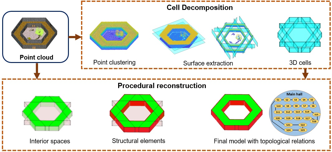
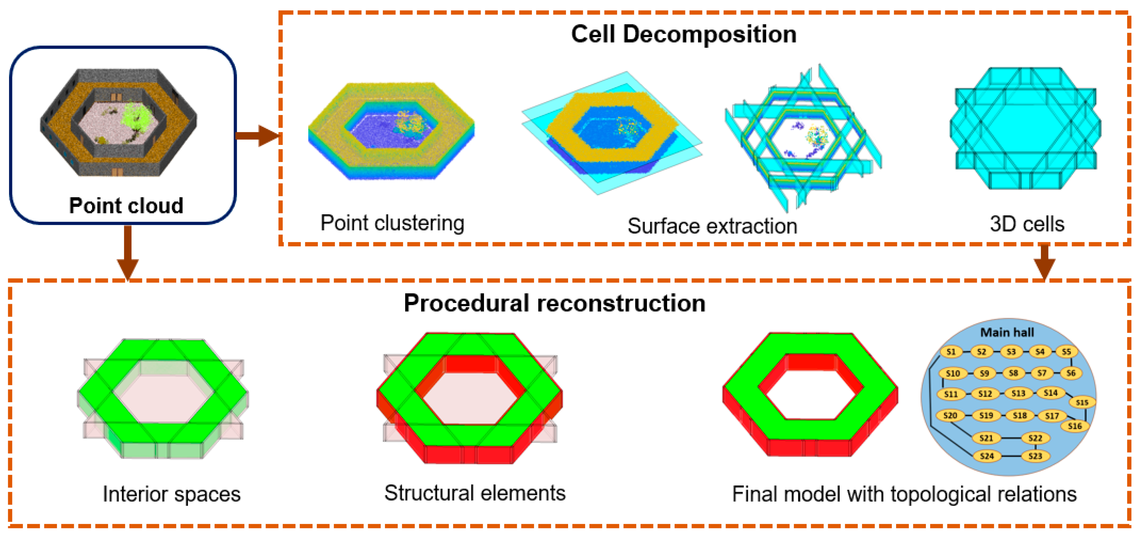
As shown in Figure 1, the proposed approach contains two main steps: space decomposition and procedural reconstruction. In the first step, the potential planar-surfaces of structural elements (e.g., wall surfaces) are extracted from clustered points of the point cloud, and the surfaces are then used to decompose the indoor environment into a set of 3D cells. Intuitively, building surfaces usually separate different interior elements (e.g., between spaces and walls). Thus, different types of interior elements (e.g., spaces and walls) are likely to be represented as separated cells. The point cloud and the 3D cells are then used in the reconstruction process.
In the procedural reconstruction, a 3D layout of the building interiors is derived based on a combination of a shape grammar, hereafter referred to as indoor grammar, and a stochastic process, i.e., the rjMCMC algorithm. The indoor grammar is an extension of the Manhattan grammar proposed in Reference [11] to be applicable to both Manhattan and non-Manhattan designs. In addition to the iterative application of placement, classification, and merging processes [11], we further include a splitting process and a reclassification of nonterminal shapes in the derivation of the model. This facilitates reversible production, which provides the ability to correct modelling errors.
The modelling procedure starts with a reconstruction of interior spaces (i.e., rooms and corridors). The shape grammar allows reconstruction of the model in a hierarchical structure by using not only the geometric information but also the knowledge about structural arrangement, semantic information, and topological relations, owing to inherent characteristics of a shape grammar in maintaining topological correctness between the elements. The rjMCMC algorithm guides the automated application of grammar rules, which induces the next proposed model among several matching possibilities from the current existing elements of the model, hereafter referred to as the current state. The reconstructed model is further evolved by a production of the structural elements (e.g., walls, ceilings, and floors), which are derived based on the geometry and their topological relations with interior spaces. Finally, the exterior cells within the scope (i.e., bounding box) of the environment, which are neither interior spaces nor structural elements, are labelled.
3.1. Space Decomposition
The input point cloud is first clustered into three groups: horizontal, vertical, and others. A dual process, consisting of local-scale extraction and global refinement, is then applied for the extraction of surfaces of horizontal and vertical structures separately. The cell decomposition of an indoor environment is created as an arrangement of the extracted structures. The remainder of this section explains the three steps in detail.
Point clustering: The point cloud is clustered into three groups, i.e., horizontal points representing the horizontal structures (e.g., ceilings and floors), vertical points representing the vertical structures (e.g., walls), and others belonging to noises and clutter, based on their normals. The goal is to eliminate irrelevant points (e.g., noises and clutter) in the extraction of building surfaces as well as in the reconstruction of the final model.
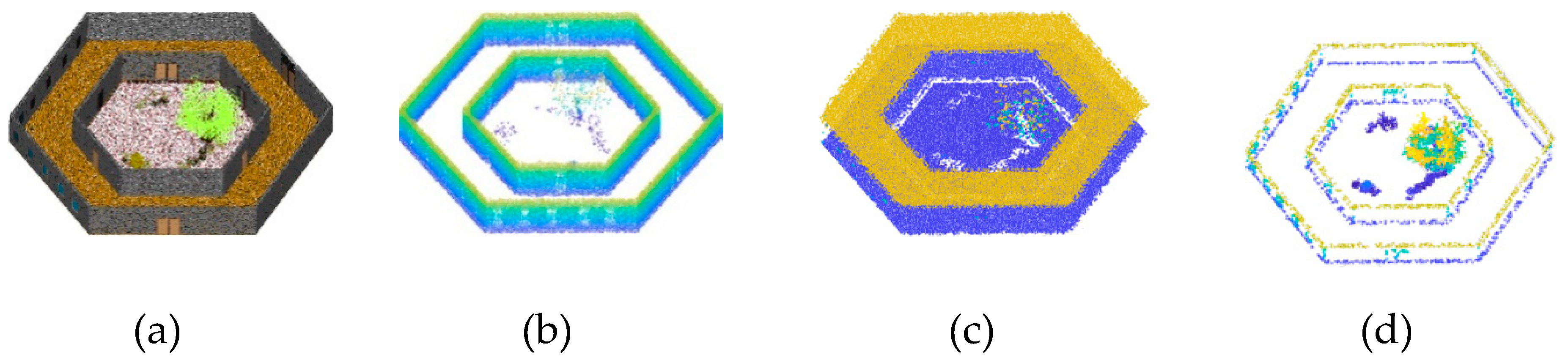
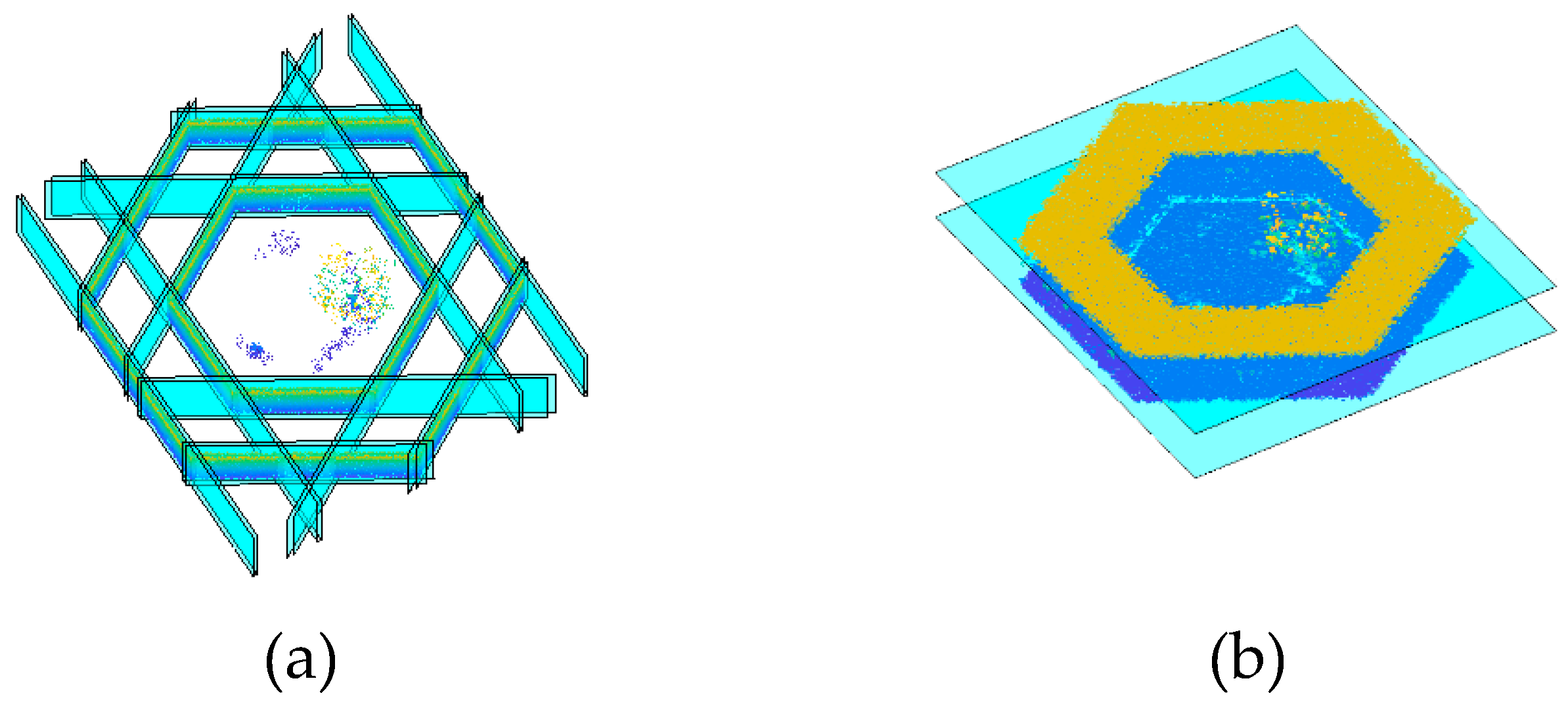
Given that point clouds captured by various lidar sensors normally have an upright orientation, a point is classified as horizontal or vertical if its normal is parallel with the horizontal direction and vertical direction , respectively, up to a small deviation (e.g., degrees). The points which belong to neither horizontal nor vertical groups are classified as others, and these points are then excluded in further processes. Figure 2 shows an example of point clustering, which demonstrates the exclusion of a considerable amount of clutter from the points representing building structures (i.e., vertical and horizontal points) of a hexagonal building.
Surface extraction: A random sample consensus (RANSAC)-based plane-fitting algorithm [36] is used for generating reasonable structure surfaces of the building interior. In this step, we extract horizontal structures and vertical structures from horizontal and vertical clusters, respectively, to lessen mutual influences between them. However, the process may still produce undesired surfaces which have arbitrary orientations and a small number of supporting points when applied to large buildings and heterogeneous point clouds. To tackle this problem, we propose a multi-scale surface extraction, including a local-scale extraction and global refinement.
Local-scale extraction: The building surfaces are initially extracted at a local scale, which is at voxelized structures of horizontal and vertical data. The voxel size is empirically defined and suggested to be set as an ordinary room’s dimensions, e.g., 3 to 5 meters. By this way, it facilitates the extraction of building surfaces from a building part that will not be influenced by the points belonging to the other parts of the building. Thus, it reduces the involvement of irrelevant elements in the extraction of a building surface. A valid vertical or horizontal building surface is in the vertical or horizontal directions, respectively, and it contains a certain amount of supporting points. Figure 3 illustrates the surface extraction at the local scale from vertical points of the hexagonal building.
Global refinement: The initial surface segments extracted locally are iteratively refined in order to generate an optimal set of surfaces for a building interior. Two local surfaces , which are parallel with each other up to a small threshold angle ) and have a threshold distance between them ) are likely to represent the same building structure and, therefore, will be merged and replaced by a new surface. In general, the thresholds do not have a significant impact on the extraction result: the angle is recommended to be less than 10 degrees, and the threshold distance should be no larger than the nominal accuracy of the data points. The distance between two surface segments distance is defined as the minimum point-to-plane distance [37] between the supporting points of one surface to the other. The merged surface is fitted from the combined set of supporting points of its two component surfaces. The refinement is repeated until no more surfaces can be merged. Figure 4 shows the final extracted surfaces of the hexagonal building after the refinement.
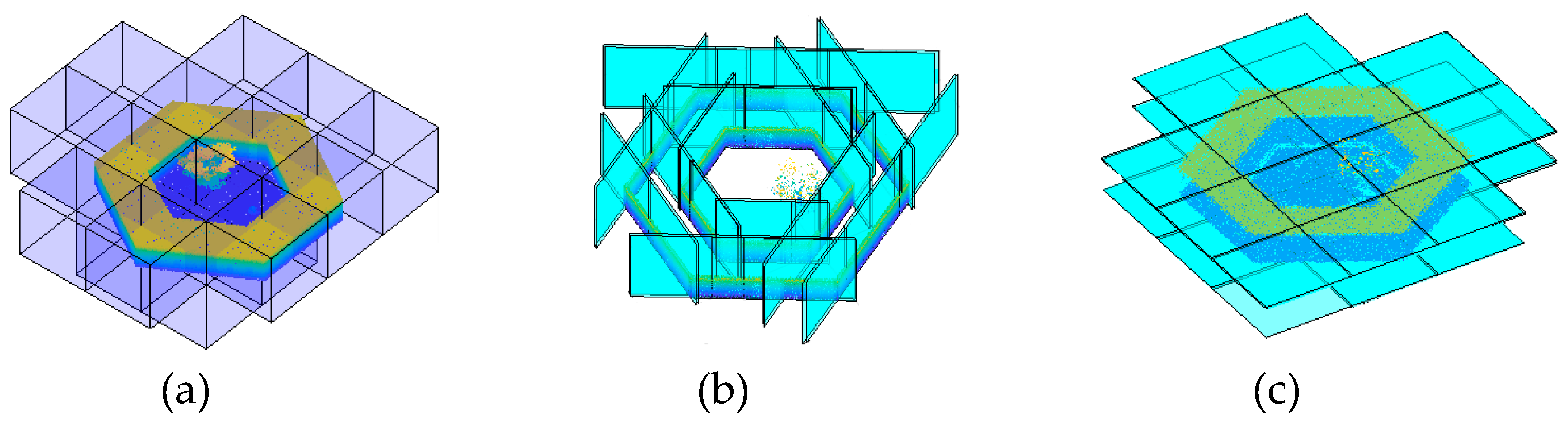
Cell decomposition: An arrangement of the extracted horizontal and vertical surfaces decomposes the building interior into a set of 3D cells. The intersections between all vertical surfaces with a horizontal structure, such as the floor surface of the building, are first computed. These line intersections are then used to partition the horizontal structure into a set of 2D cells using the 2D arrangement [38] of the Computational Geometry Algorithms Libraries [39]. These horizontal 2D cells are then extruded in vertical directions and intersected with the other horizontal surfaces (e.g., the ceiling) to generate 3D cell decomposition of the building interior. Figure 5 illustrates the cell decomposition of the hexagonal building from its vertical and horizontal surfaces.
3.2. The Indoor Shape Grammar
The indoor shape grammar is an extension of the shape grammar proposed by Tran et al. [11] to model both Manhattan and non-Manhattan world indoor environments. The extension includes a new shape definition, extended grammar rules, and the integration of a stochastic process to the production procedure using the rjMCMC.
3.2.1. Shapes
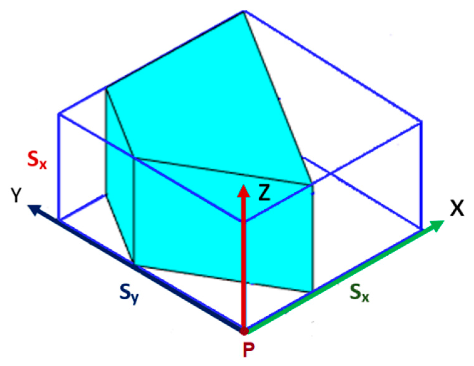
In general, a shape grammar contains a finite set of shapes, including a starting shape and nonterminal and terminal shapes [40]. In the indoor shape grammar, a shape is a polyhedron: it is assigned a unique identifier id and consists of 4 elements, i.e., a scope (i.e., bounding box), geometry (i.e., geometric attributes), semantics (i.e., semantic attributes), and topological relations (i.e., topological attributes). Similar to Reference [13], the scope is defined as the oriented bounding box of a shape, represented by a corner point P; three orthogonal vectors , indicating its orientation; and a scale vector , representing the dimensions along the 3 orthogonal directions. The shape geometry is described with a boundary representation , where V is the set of vertices and F is its bounding faces. Figure 6 shows an example of a shape with its scope (blue bounding box) and geometry representation (cyan bounding surfaces).
Similar to that in Reference [11], the semantic attribute implies the type of a shape, which can take one of three values (interior space, exterior, and wall), and the topological attributes indicate the shape’s adjacency, connectivity, and containment relations. The starting shape is a unit scope with the point P located at the origin of the local coordinate system, and the unit scale represents the dimensions along the x-, y-, and z-axes. The unit scope has empty geometry, no semantic information, and topological relations.
3.2.2. Grammar Rules
The grammar rules define operations on shapes, which transform antecedent shapes into subsequence shapes. We propose 8 grammar rules categorized into three types: geometric transformation, semantic conversion, and topological relation establishment rules. The grammar rules are defined in the following form:
The antecedent shapes are nonterminal shapes, while the subsequent shapes can be either nonterminal or terminal shapes. The rule is applied on the condition cond and is selected with probability prob, which is automatically learned during the derivation of the 3D models. The detail of this derivation process will be described in the next section.
Geometric transformation rules: The rules are operated on the shapes’ geometries and, therefore, transform the geometry of a model. The applications of the rules can also involve varying the number of shapes constituting a model. The place and merge rules are inheritably modified from our previous work [11], while the split rule is new and is defined to allow reversibility of the reconstruction.
- (1)
- Place rule:
The place rule places a nonterminal shape N into the scope of the indoor environment by transforming the starting shape (the unit scope) using a set of transformation parameters H. The transformation H consists of the scope information of the shape N and its geometry representation. The scope is determined by a translation vector and a rotation , indicating the location of the shape bounding box, coupling with a scale vector , and encoding its dimensions. The shape geometry is represented with a set of vertices and bounding faces , which are obtained from the 3D cell decomposition of the building. If no cell can be found in the environment, then H is an empty set and the rule cannot be applied.
- (2)
- Merge rule:
The merge rule replaces two nonterminal shapes and with their union B on the condition that they are both of type interior space and are in a connectivity relation.
- (3)
- Split rule:
The split rule is the reciprocal of the merge rule. The rule applies a split to a shape and then replaces it with two component shapes and . The and must be the antecedents, and shape B is the subsequent of a previous application of the merge rule.
Figure 7 shows an example of a reversible process by application of the merge and split rules.
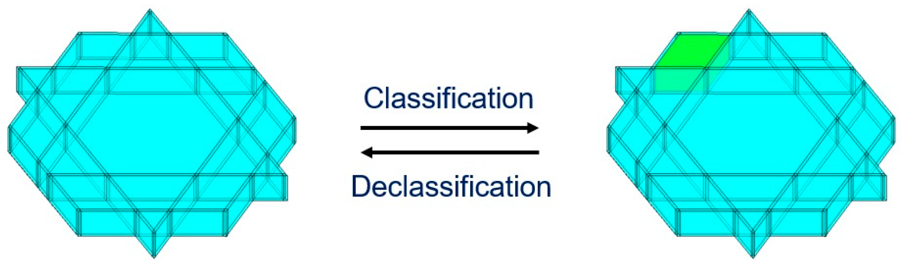
Semantic conversion rules: These rules operate on the semantic information of nonterminal shapes without changing their geometries or number of shapes in a model. The semantic conversion rules contain two reciprocal rules: classification and declassification rules.
- (1)
- Classification rule:
The classification rule assigns a nonterminal shape N, which has no semantic information (i.e., type is empty ()) and a certain type (i.e., wall, interior space, or exterior). The condition cond and probability prob of the rule are automatically learned using the stochastic process using rjMCMC during the reconstruction of interior spaces, which will be detailed in the next section. Meanwhile, the labelling of structural elements and exteriors are inferred from their geometries and topological relations. For example, a wall should be in an adjacency relation with interior spaces and the vertex-to-surface distances [37] between its vertices and the adjacent surface should not be larger than the wall thickness of the building in accordance with predefined knowledge of the building architecture.
- (2)
- Declassification rule:
The declassification rule is a reversible process of the classification rule. The rule nulls the type attribute of a nonterminal shape N. Similar to the classification rule, the condition cond and the probability prob can be automatically learned during the reconstruction of interior spaces (detailed in Section 4).
Figure 8 illustrates a reversible process involving classification and declassification of an interior space.
Topological relation rules: The three topological rules are defined to establish the three topological relations between shapes, consisting of adjacency, connectivity, and containment relations. The condition to invoke the rules is similar to that in Reference [11]. However, in this paper, the rules are assigned a probability prob for its application, which can be learned during the reconstruction process.
- (1)
- Adjacency rule
The adjacency rule establishes the adjacency relation between two nonterminal shapes and . Prior to the reconstruction of structural elements, the two nonterminal shapes are adjacent on the condition that they share a common face. After the modelling of structural elements, two final interior spaces are in an adjacency relation if there is a common wall between them.
- (2)
- Connectivity rule
The connectivity rule establishes the connectivity relation between two nonterminal shapes and . Before the reconstruction of structural elements, two nonterminal interior spaces are connected on the conditions that they are adjacent and there is no actual surface between them. After the modelling of structural elements, two final interior spaces are in a connectivity relation if there is a common wall and the wall contains a door. Similar to our previous work [11], the doors are manually inserted to the model by updating the containment attribute of the walls.
Figure 9 shows the topological adjacency and connectivity relations established between the shapes and , which are two interior spaces of an indoor environment (Figure 9a). The adjacency relation (Figure 9b) of the shapes and is established due to a shared common face between them, and the connectivity relation (Figure 9c) is established since there is no actual physical surface between them.
- (3)
- Containment rule
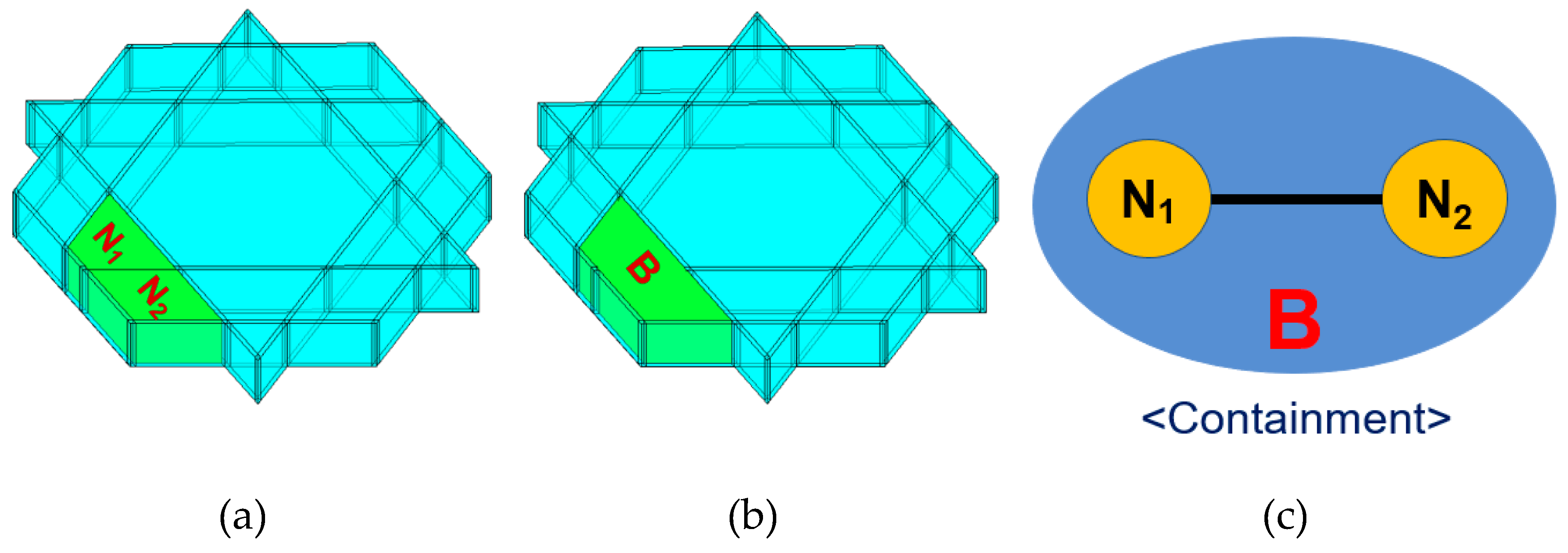
The containment attributes of two nonterminal shapes are updated via the application of the containment rule. If the shapes and are antecedent and subsequent (or vice versa) of a previously applied merge rule, their containment relations are established. In addition, the containment rule can be invoked to establish the containment relation between a door and a wall.
Figure 10 shows an example of a containment relation where shape B contains two component shapes and .
4. Procedural Model Generation Using rjMCMC
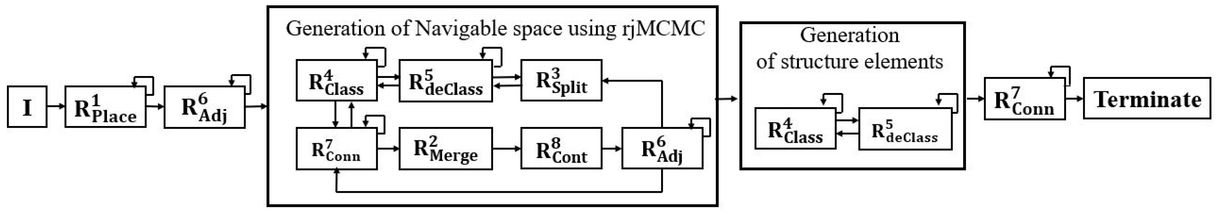
Figure 11 shows the production procedure for the generation of a 3D indoor model by iterative application of the grammar rules. An indoor model is a configuration of a finite set of shapes, which is defined by the number of shapes and the shapes’ attributes within the scope of an indoor environment. Initially, nonterminal shapes are placed into the scope of the indoor environment by iterative application of the place rule (Section 3.2.2). At this stage, each nonterminal shape N, transformed from the starting shape I (the unit scope), is represented with a scope and geometric attributes encoding its boundary representation but no semantic information and no topological relations. The probability of the rule application is set as 1 in the case that the shape’ geometry is totally matched with a cell’s geometry created from the 3D cell decomposition. If no such 3D cell can be found, then the rule cannot be applied (). Once a shape is placed in the scope of the building interior, its adjacent relations will be automatically established with its neighbours, which share a common face.
The reconstruction of the building interior then proceeds with a search for an optimal configuration of interior spaces (i.e., rooms and corridors) in the model . In this step, we aim at maximizing the model fitness to the input point cloud , while maintaining the model plausibility and its simplicity. In other words, we search for the most probable model given the data ) based on a stochastic approach using rjMCMC sampling with the Metropolis–Hastings algorithm [16,41]. The rjMCMC algorithm simulates random walks from the current model to the next proposed configuration with a capacity to cope with the variability of the number of shapes in each model configuration. The transition from a current state to the following configuration is decided by both the model probability ), a transition probability , and an acceptance probability as defined in Equation (10). The description of the model probability and the transition kernel are detailed in the following sections.
A proposed transition is accepted if the acceptance probability is larger than a random number , where is the convergence factor [41]. This triggers the application of grammar rules, for which guarding conditions are satisfied, in order to generate a new configuration. The acceptance probability is assigned as the application probability of the triggered rules. The convergence factor provides the flexibility in searching for the optimal model either in a model subspace () or in the whole space of models as default () [8]. In general, the application of grammar rules in the reconstruction of interior spaces is in a stochastic order. However, in order to maintain the global plausibility of the model and the model conformity to architectural principals, the process requires to follow certain procedural priorities. For example, once a new interior space is added to the model, its topological relations (i.e., adjacency and connectivity) must be established spontaneously. Likewise, when two connected interior spaces are merged together to form a new space, the containment rule must be applied next to establish the containment relation between the new merged space with its components. The reconstruction process of interior spaces is final when the number of the random walks in the model space of the indoor environment reaches a predefined limit. The final model will be selected among the models with the highest model probabilities given the input data. At this stage, the geometry transformation rules are no longer applied in the reconstruction process.
The reconstructed interior spaces are then taken into account for the generation of structural elements. The semantic conversion rules are applied to assign semantic information (e.g., walls and exteriors) to non-interior spaces which have no semantic information, followed by the application of topological relation rules to establish the topological relations among reconstructed shapes (i.e., final interior spaces and walls) of the model. At this stage, the probability of the rule application is set as 1 () if their guarding conditions are satisfied. Otherwise, the probability is set to 0 (). Once all the shapes are labelled and no more topological relations can be established, all the reconstructed interior spaces, structural elements, and exteriors are terminal shapes.
4.1. Model Probability
The model probability ) indicates the probability of a model configuration given the input point cloud . The probability is defined to encode the prior knowledge of building architecture and to measure the model fitness to the input and the model plausibility. According to Bayes’ rule, the model probability ) is proportional to the product of the prior and the likelihood : .
4.1.1. Prior Probability
The prior of a model is defined as a joint probability distribution of the prior of the shapes comprising the model , in this case, interior spaces:
where is number of interior spaces of the model . is the prior of the shape .
Without any observed data, the prior of an interior space is derived from the geometric information and the constraints on knowledge of building architectures. We first define the width of a shape as the smaller horizontal dimension of its scope (i.e., the bounding box).
Intuitively, an interior space should have a large width in comparison with a structural element (i.e., walls). We, therefore, assign the prior of an interior space to , if the shape has a width larger than the maximum wall thickness. Otherwise, the prior is set to . For the special case when the model has no interior space, the prior of the model is set to .
4.1.2. Likelihood
The likelihood encodes the model fitness as well as its conformity to the input data. The model fitness is measured at both local scales for each individual shape (so-called local likelihood) and the global fitness of the whole model (so-called global likelihood). In other words, the approach facilitates the integration of both local characteristics of data and global plausibility of the model in the reconstruction of the model. We therefore define the likelihood of the model as a joint distribution of the local likelihood and the global likelihood :
Local likelihood: The local likelihood is computed based on the interpretation from local characteristics of data points enclosing each individual shape of the model. The local likelihood of a model is a joint distribution of the likelihood of each interior shape to its enclosing data points. Intuitively, an interior shape is likely to contain points on its top surfaces (i.e., ceiling) [10]. We therefore define the likelihood of each interior shape as the coverage of its top surfaces [42], which is computed as the ratio between the alpha-shape area covered by the shape’s data points [43] and the area of the top surface. The local likelihood of the model, therefore, is formulated as follows:
where is the number of interior spaces of the model . denotes the area of a surface of a shape. Meanwhile, denotes the area of the building surface, which is covered by points.
The local likelihood ranges from 0, implying that, in the proposed model, there is at least one interior space with no supporting points, to 1, implying that all the interior spaces are covered totally by the input data points.
Global likelihood: The global likelihood measures the fitness of the whole model as well as its general plausibility with respect to the entirety of the input point cloud . The global likelihood is defined as the combination of three data terms, i.e., (1) horizontal fitness , measuring how good the horizontal structure fit with the horizontal points ; (2) vertical fitness , measuring the fitness of the vertical structures to the vertical points ; and (3) model plausibility , indicating the reliability and conformity of the model with respect to the data (i.e., both horizontal and vertical points). Depending on the intrinsic characteristics of data such as the level of incompleteness, noise, or clutter, the contribution of each data term to the global likelihood varies. The global likelihood, therefore, is formulated as follows:
where , , and are the normalization factors weighting the contribution of the data terms to global likelihood. The normalization factors must satisfy the condition .
Horizontal fitness: The horizontal fitness is computed as the normalized horizontal coverage of the model . The horizontal coverage of a model is the area of the top surfaces of its interior spaces (i.e., rooms and corridors) covered by horizontal points . The normalization is the ratio between the model’s horizontal coverage and the horizontal areas of the building, which are covered by the horizontal points . In other words, the more horizontal surfaces covered by the horizontal points, the higher the horizontal fitness of the mode model . We formulate the horizontal fitness of a model as Equation (15) below:
where denotes the alpha-shaped area covered by points.
Vertical fitness: Similar to horizontal fitness, the vertical fitness of the model is computed based on its vertical coverage. The coverage is measured as the surface area of vertical structure (i.e., wall surfaces), which is covered by the vertical data points summed over all interior spaces of the model. The vertical fitness is formulated as the normalization of the model’s vertical coverage, which is defined as the proportion of the vertical coverage of the model to the vertical coverage of the building. The horizontal fitness of the model M is formulated as Equation (16):
Model plausibility: The general plausibility of model with respect to the input point cloud is computed based on the areas covered by both horizontal and vertical points, which fall inside the interior spaces and, therefore, do not represent the horizontal or vertical structures. The more horizontal and vertical areas covered by these inside points, the lower the plausibility of the model. The model plausibility is therefore formulated as follows:
where is the horizontal and vertical points which fall inside an interior space .
The model plausibility may be influenced by the indoor environments, which have a high level of clutter. In these cases, the plausibility should have only a small contribution to the global likelihood of the model, and it can be adjusted by lowering the value of its normalization factor in Equation (14).
4.2. Model Transition
The transition kernel represents the probability for the change from the current model to the next proposed model . In the reconstruction of interior spaces, there are four possible changes in the configuration of a model [8], including adding a new interior space or removing an existing interior space by application of classification or declassification rules as well as by splitting an interior space into two components or by merging two spaces into a merged one by invoking the split rule and merge rule, respectively. These changes will cause the variation in the number of shapes configuring the model. In addition to maximizing the fitness of the model with respect to the data, which are encoded via the model probability (Section 4.1—Model Probability), our goal is to reconstruct a compact model with low complexity. The concept of minimum description length [44] is therefore adopted to define the transition kernel. The description length of the model is described as the number of interior spaces. In other words, the model of a building interior, which has a smaller number of interior spaces, is favoured as being more likely than a complex one with many small spaces. This strategy ensures that the final model is formed as the union of the final interior spaces rather than separated components.
We formulate the complexity of a model as follows:
where n is the number of interior spaces in the model M. In a special case, , when .
The transition kernel is defined as follows:
where is a smoothing coefficient. To set the value of , we consider the following three cases: case 1, the current model contains the same number of interior spaces as the proposed model ; case 2, contains fewer spaces than ; and case 3, contains more spaces than .
5. Experiments and Results
5.1. Experiments
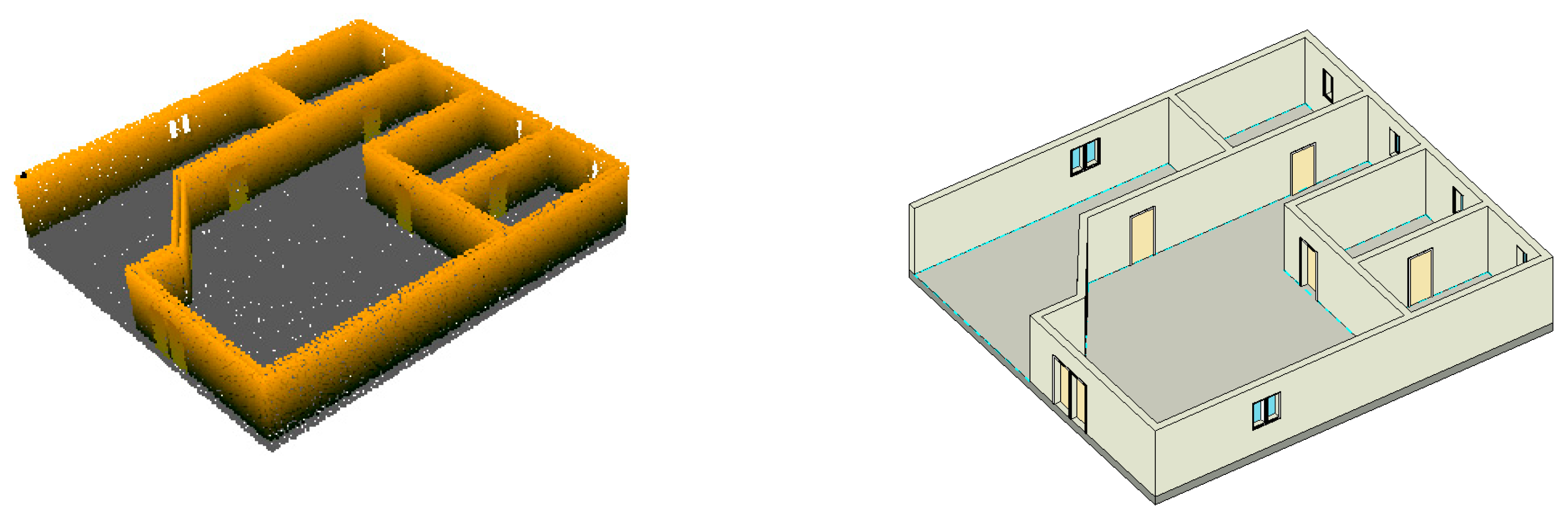
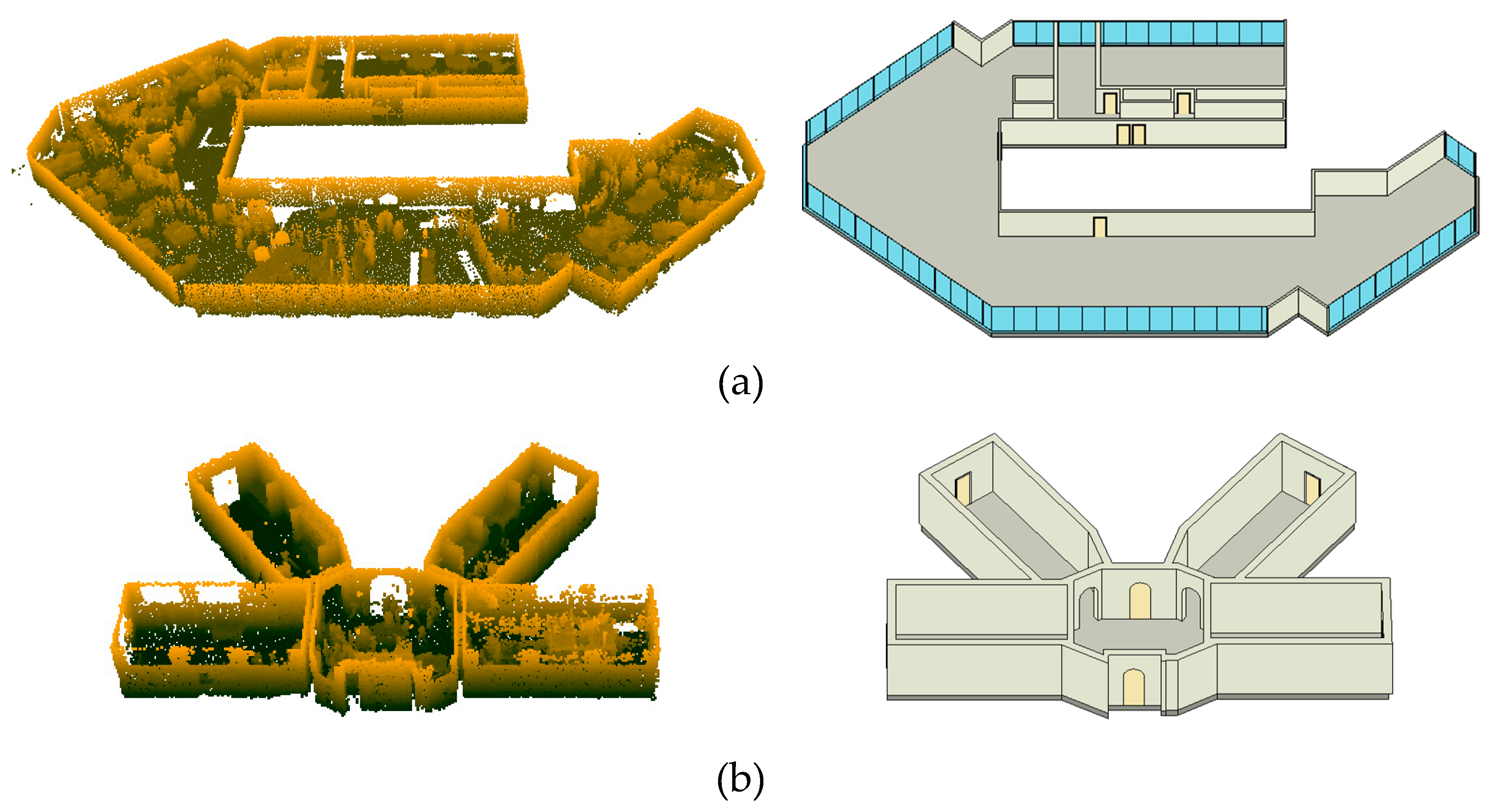
The proposed approach was implemented in MATLAB and C++ on a personal computer (i7-7500U GPU, 2.7 GHZ, with 16.0 GB memory). The CGAL C++ library was used in the cell decomposition process. Several experiments were carried out using a synthetic point cloud and two real point clouds to evaluate the feasibility of our approach in the reconstruction of indoor environments, which contain both Manhattan and non-Manhattan structures. The synthetic point cloud (hereafter referred to as SYN) simulates a simple residential house consisting of a common room, 3 private rooms, and an open indoor space with no clutter. The point cloud has a random error of 5 mm and its average point spacing is 5 cm. The real point clouds capture a research lab’s office (hereafter referred to as Office) and an art museum (hereafter referred to as Museum) at the University of Melbourne. The research lab’s office, which has a common structure of a modern office, contains a large workspace with an irregular shape, a kitchen, a printing room, a large meeting room, and a long corridor. The museum contains a reception hall which connects with four other exhibition rooms. The point clouds were captured by a Zeb Revo RT handheld laser scanner with a nominal accuracy of 3 cm. The real buildings contain a high level of clutter, which therefore occlude the building surfaces from the scanner. Each data set has a ground truth BIM model, which is used for quality evaluation of the reconstructed model.
Figure 12 shows perspective views of the synthetic point cloud and its ground truth model, and Figure 13 shows the point clouds and the ground truth models of the real environments.
In Table 2, we list the parameters used in the reconstruction process. The max wall thickness is defined based on prior knowledge of the indoor environments. Meanwhile, appropriate values for the convergence factor, normalization, and smoothing coefficients are experimentally found in relation with the quality of input data (i.e., the level of noise, the completeness of data, and the level of clutter). For the convergence factor, a higher value is more appropriate for data with lower quality so that it can help to avoid undesired model configurations in the sampling process. The smoothing coefficient is set such that it favours the applications of the merging rule over the splitting rule. The normalization factors are set equally to indicate an equal consideration of the level of completeness in both horizontal and vertical surfaces and the level of clutter of the input data in the modelling process.
The proposed approach was also evaluated using the ISPRS indoor modelling benchmark data sets [45]. Although these data sets mostly contain Manhattan world structures, they represent large and complex indoor environments with various levels of noise, clutter, and occlusions and were acquired by different types of laser sensors, including both terrestrial (e.g., Faro Focus) and mobile (e.g., Zeb and Viametris) laser scanners.
5.2. Results
5.2.1. Model Reconstruction
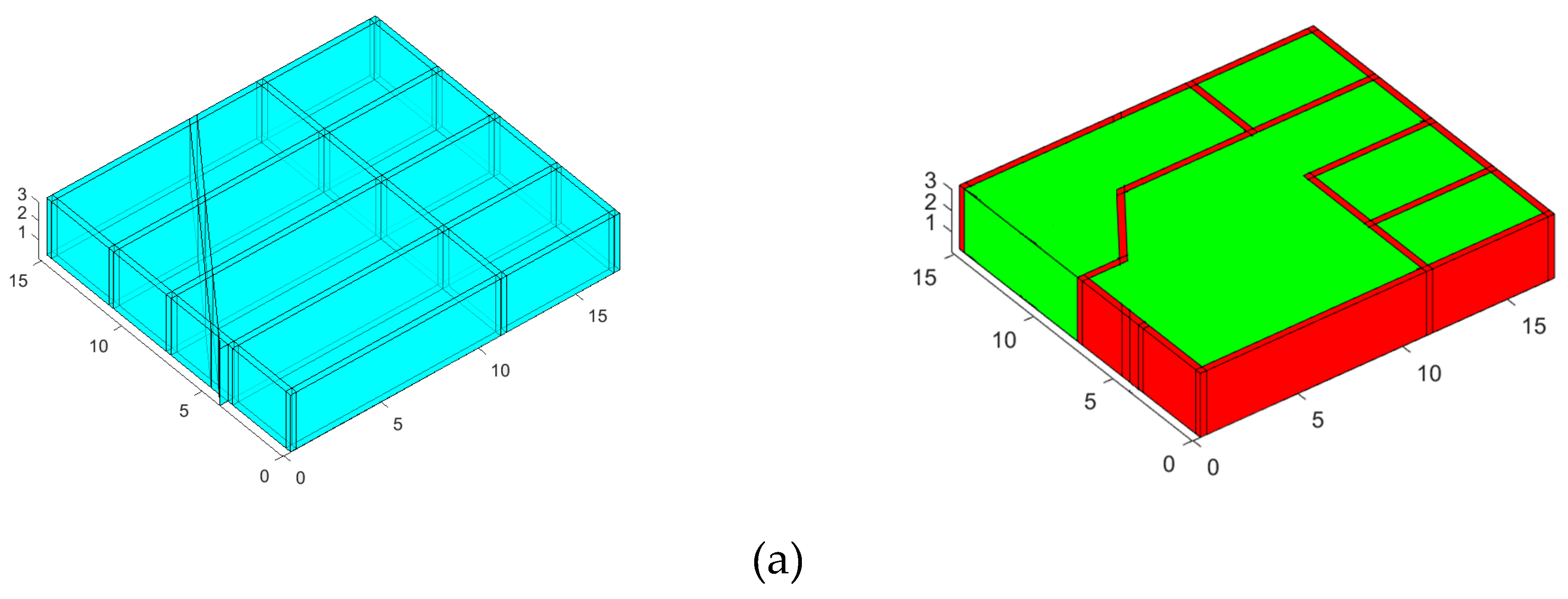
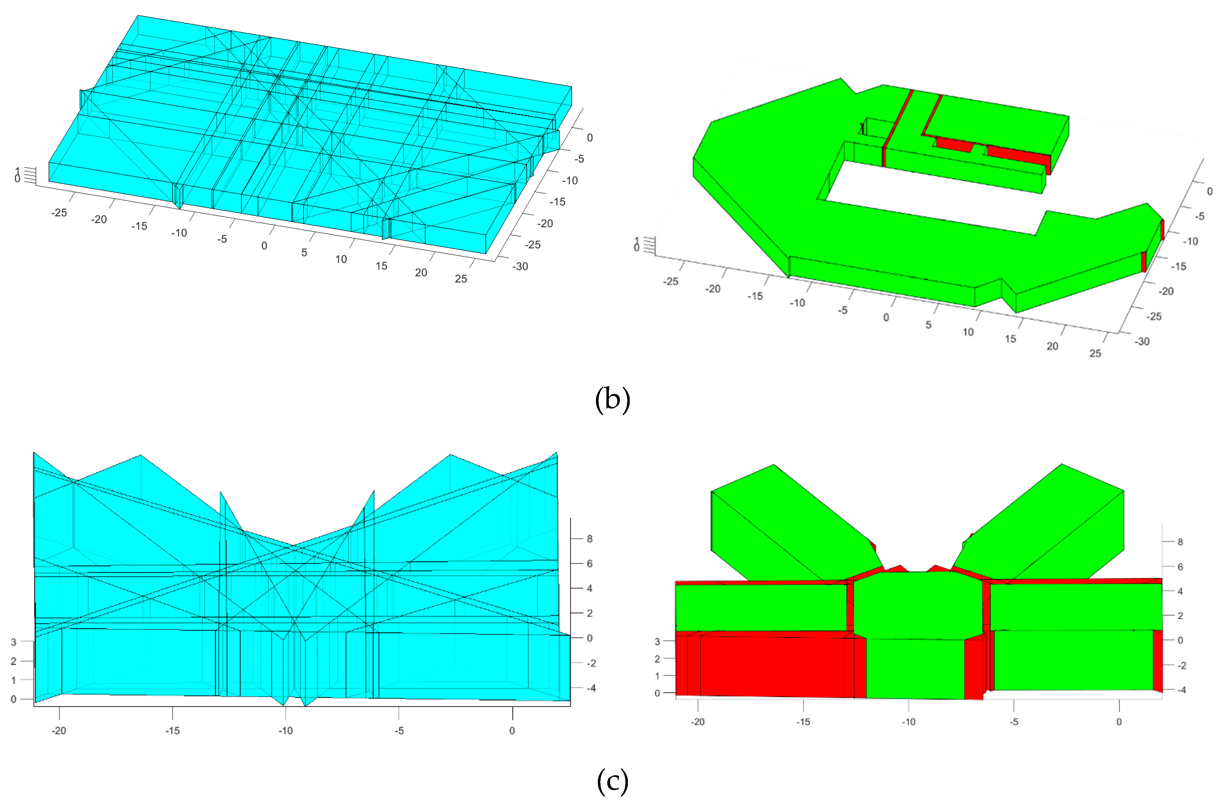
The proposed approach generally works well on the three test data sets. Figure 14 shows the cell decompositions and the reconstructed models of the synthetic environment SYN and the two real buildings, i.e., Office and Museum. The environments are partitioned into a set of arbitrary polyhedral cells. The final models contain not only the final interior spaces (i.e., rooms and corridors) and volumetric structural elements (i.e., walls) but also exterior spaces which are located within the scope of the environments. Due to the lack of data representing exterior surfaces of walls, the exterior walls are not reconstructed in the Office model. Meanwhile, parts of the exterior walls are present in the Museum model based on the interpretation from the data points captured in other parts of the building and from knowledges of building architectures, such as the max wall thickness and their topological relations with interior spaces. Both exterior and interior walls are reconstructed in the SYN model as the input data contain data points representing them. Nonterminal shapes are also modelled as inactive elements in the final model, which allows later querying hierarchical structures of shapes at different granularities. Akin to exterior spaces, these inactive elements are excluded from visualization.
5.2.2. Quality Evaluation
Quantitative evaluation of the reconstructed models was carried out by using the evaluation approach proposed by Tran et al. [3]. Since the volumetric walls are represented by both visible surfaces and interpreted surfaces [3], the evaluation is based on the comparison between the bounding surfaces of interior spaces (i.e., rooms and corridors) in the reconstructed model with the visible surfaces of the structural elements (i.e., walls, ceilings and floors) bounding the corresponding interior spaces of the ground truth.
The quality of the reconstructed models is measured in terms of three quality metrics, i.e., completeness (Mcomp), correctness (Mcorr), and accuracy (Macc) for the buffer size b and the cutoff distance r in the range [1 cm, 10 cm]. The completeness aspect indicates to what extent the geometric elements of the ground truth are present in the reconstructed model, while the correctness aspect expresses to what the extent the elements in the reconstructed model are present in the ground truth. These quality metrics are defined as follows [3]:
where denotes the buffer with size b created around a ground truth surface Rj and where n and m are the number of surfaces in the reconstructed model S and in the ground truth R, respectively. The operator |.| denotes the area of the surface, and denotes the orthogonal projection operation of a surface in the reconstructed model on its corresponding surface in the ground truth.
The accuracy measures the closeness between the ground truth and the reconstructed model and is defined based on Euclidean distance between the dense points representing the ground truth and the closest surfaces in the reconstructed model [3]:
where is the orthogonal distance between a point of the point cloud, which represent the ground truth, and a surface plane of the reconstructed model. |.| denotes the absolute value.
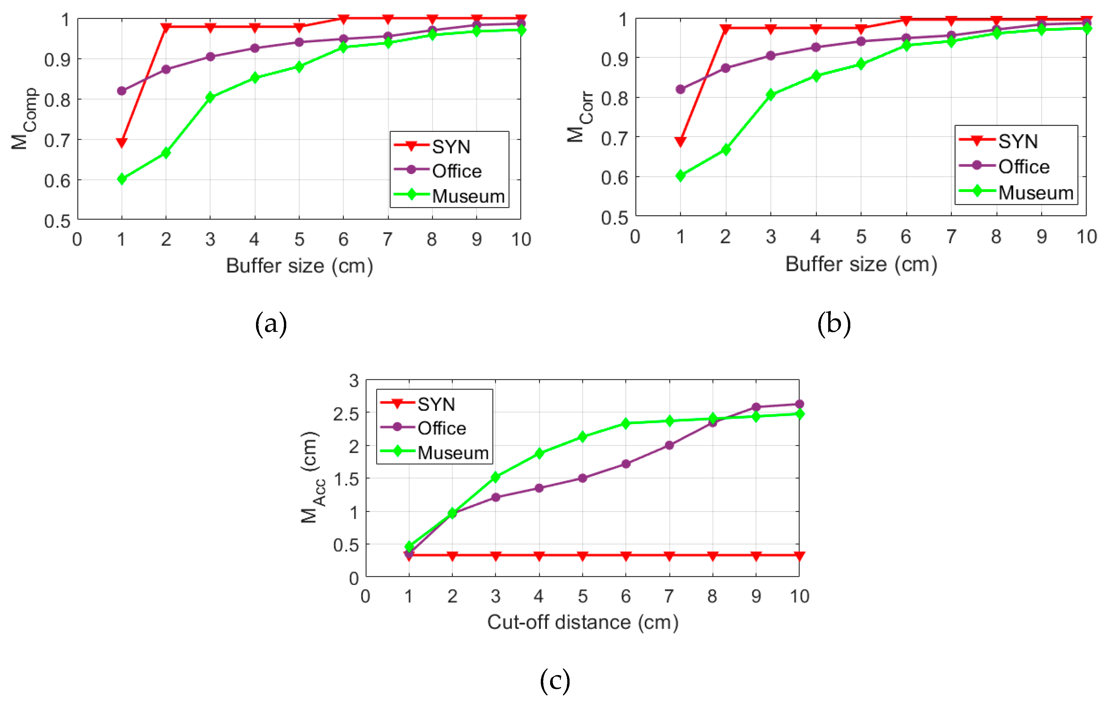
The evaluation results of the three reconstructed models is shown in detail in Figure 15.
As can be seen in Figure 15, the quality curves reveal that the models of both the synthetic environment and the real buildings are reconstructed with high completeness ( at ) and correctness ( at ). It can be verified by visual inspection that the majority of the ground truth elements are present in the reconstructed models. The SYN model is reconstructed with high accuracy (), which agrees with its random error. Meanwhile, the accuracy of the Office and the Museum are and , respectively.
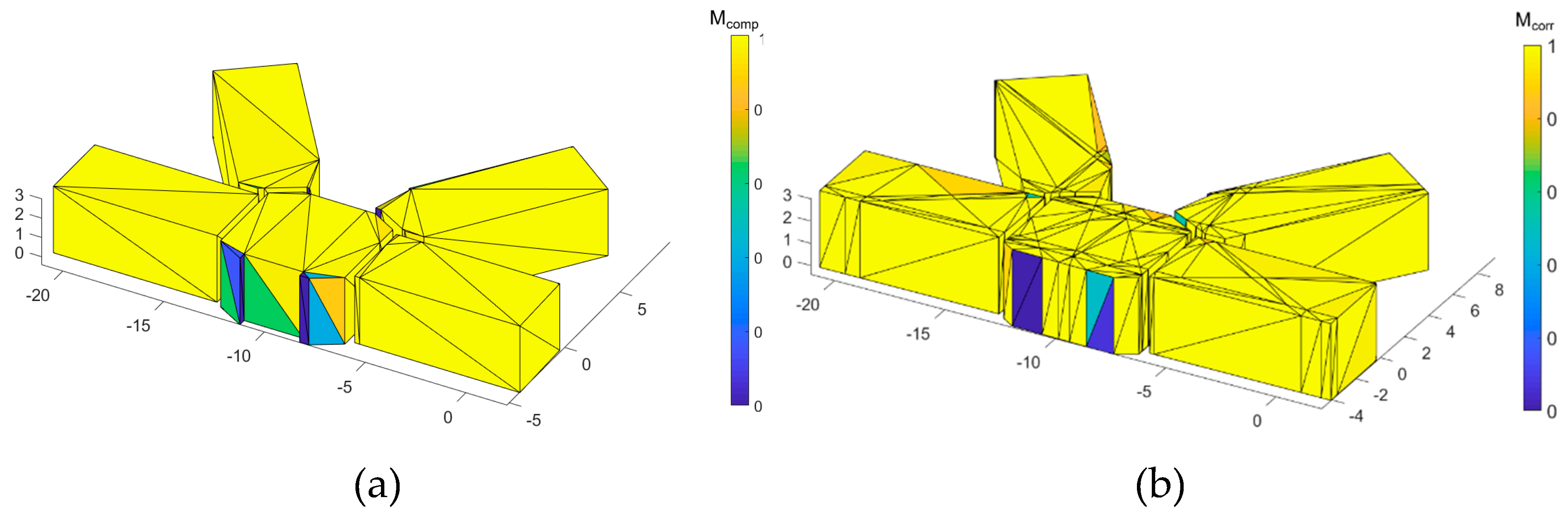
We further locate the completeness and correctness errors in order to identify the additional elements and the missing elements in the reconstructed models in comparison with the ground truths. Figure 16 illustrates the localization of the completeness and correctness errors of the Museum. The completeness and correctness errors indicate that the entrance of the Museum is not well reconstructed. Most of the surfaces (in blue colour) of this building part having low completeness () and low correctness (). These elements are therefore considered as the additional surfaces (blue) in the reconstructed model and missing surface (blue) of the ground truth in the final model.
5.2.3. Reconstruction of Topological Relations
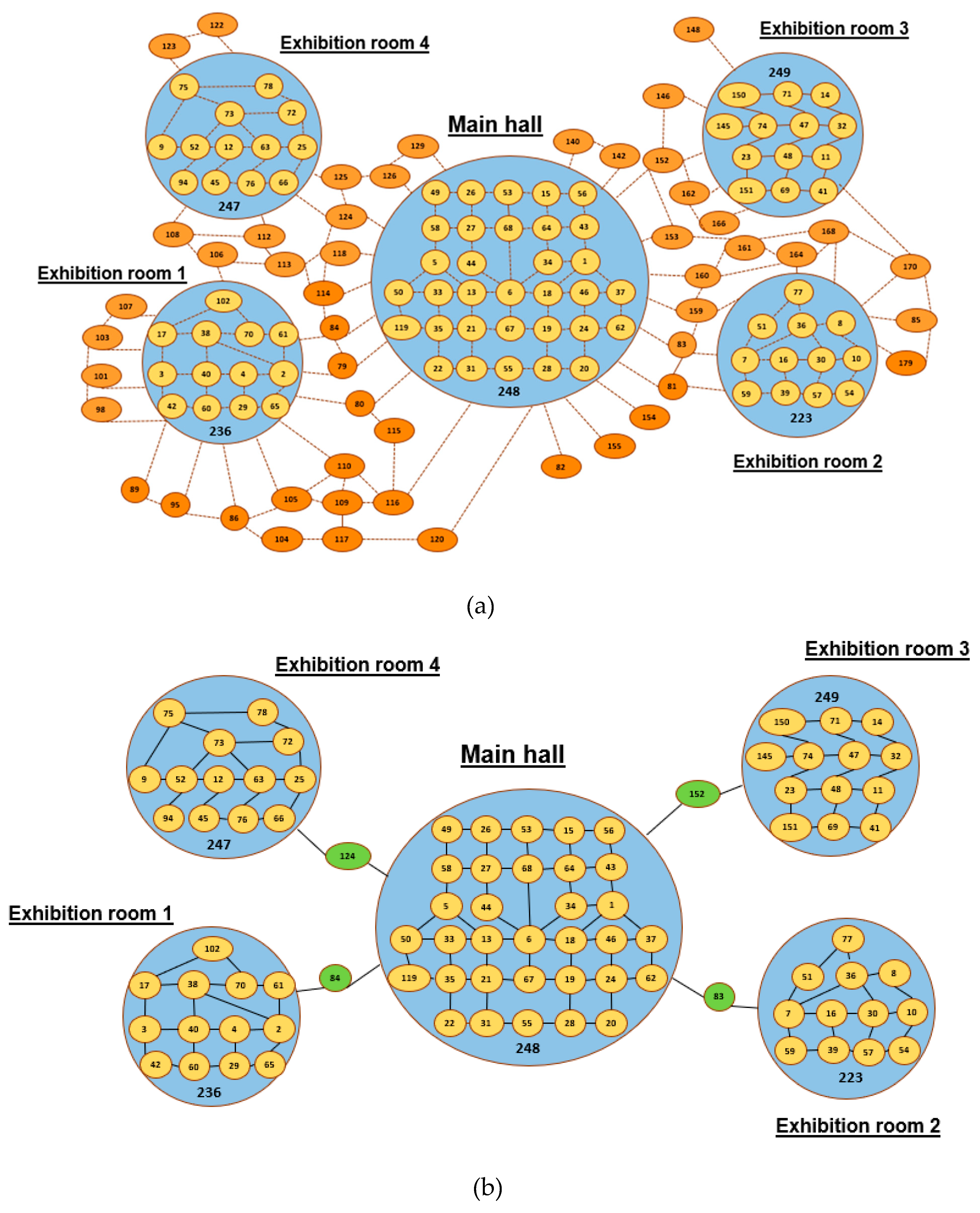
In addition to the generation of semantically rich 3D models of indoor environments, our proposed approach is able to establish the topological relations, i.e., adjacency, connectivity, and containment, between elements of the models owing to the characteristics of the shape grammar in maintaining the topological correctness. Each element is represented by its assigned unique id in the model. Figure 17 shows the reconstructed topography graphs for the Museum, which are extracted at the granularity of nonterminal spaces. The blue circles represent the containment relations between the final interior spaces (the rooms and the corridor) and their subspaces (yellow circles). The relations between the final interior spaces and their adjacent walls (brown circles) are also established. The adjacency relations are represented by brown dashed line in Figure 17a. The doors are manually inserted into the wall ids 83, 84, 124, and 152 (green circles). This can be simply done by interactively invoking the containment rules to establish the containment attribute of the walls. The connectivity relations established between both final spaces and subspaces are represented as black solid lines as shown in Figure 17b. Figure 18 shows the connectivity at the granularity of the final spaces (i.e., rooms and corridors) of the Museum.
5.2.4. Reconstruction of ISPRS Benchmark Data Set
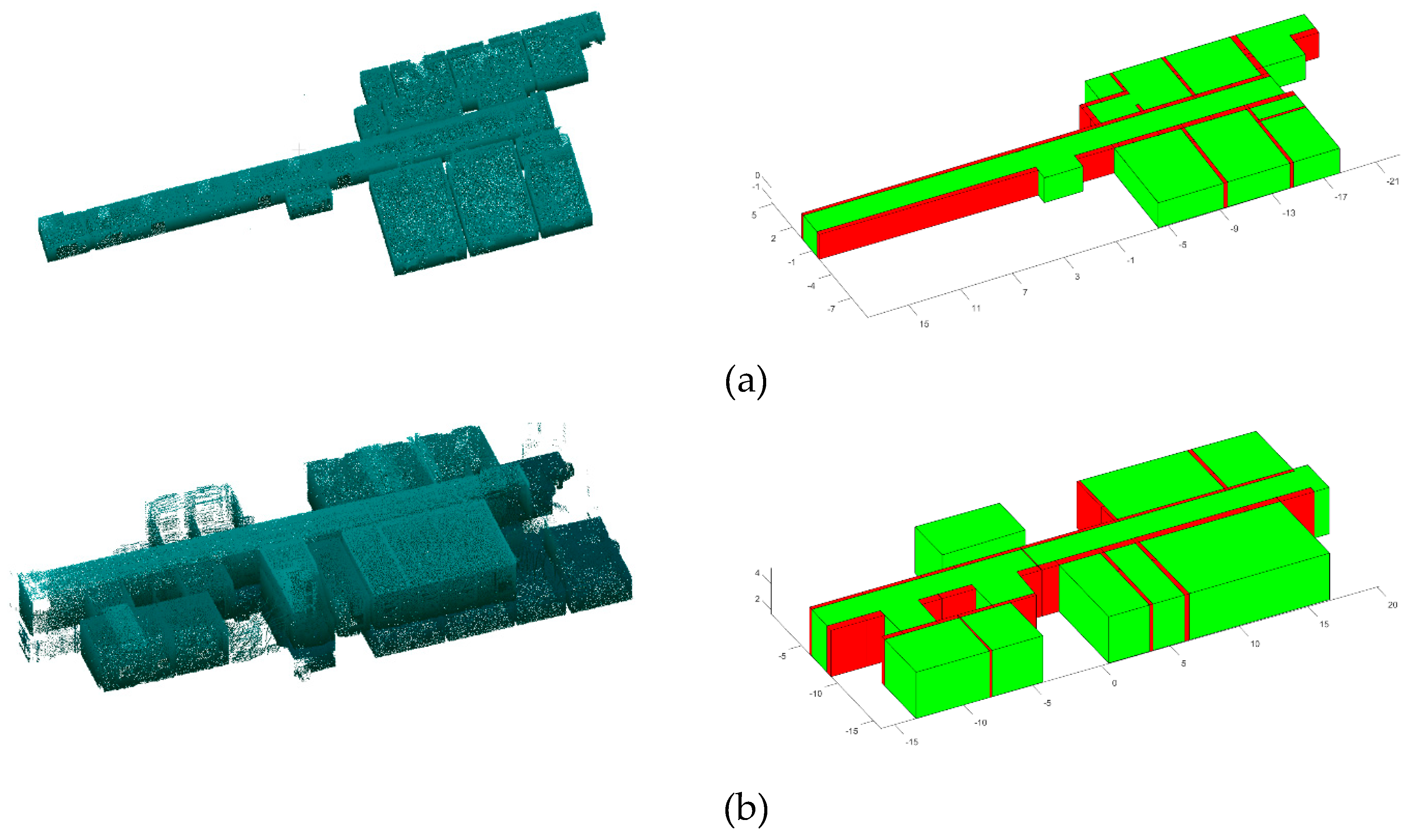
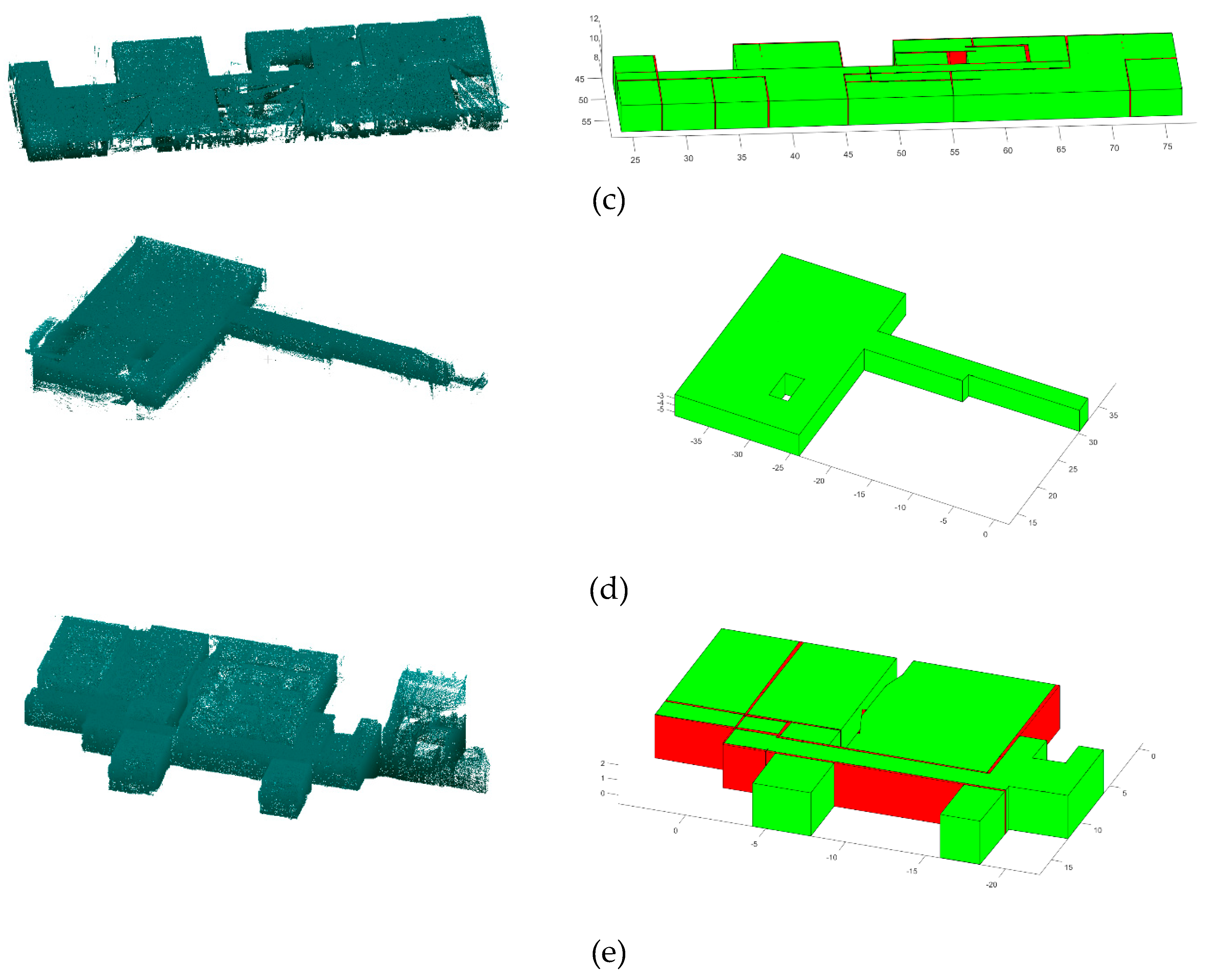
The proposed approach is evaluated on the five ISPRS Benchmark data sets, including TUB1, the 2nd floor of TUB2, Fire Brigade, UVigo, and UoM. Figure 19 shows the point clouds and the models reconstructed from the ISPRS Benchmark data sets. Visual examination of the reconstructed models indicates that most of the elements of the indoor environments are correctly reconstructed. However, these models contain several undesired elements and missing elements in comparison with the as-is condition of the environments captured in the input point clouds. For example, there are additional rooms and walls in both the TUB2 and Fire Brigade models as well as missing walls in the UVigo model.
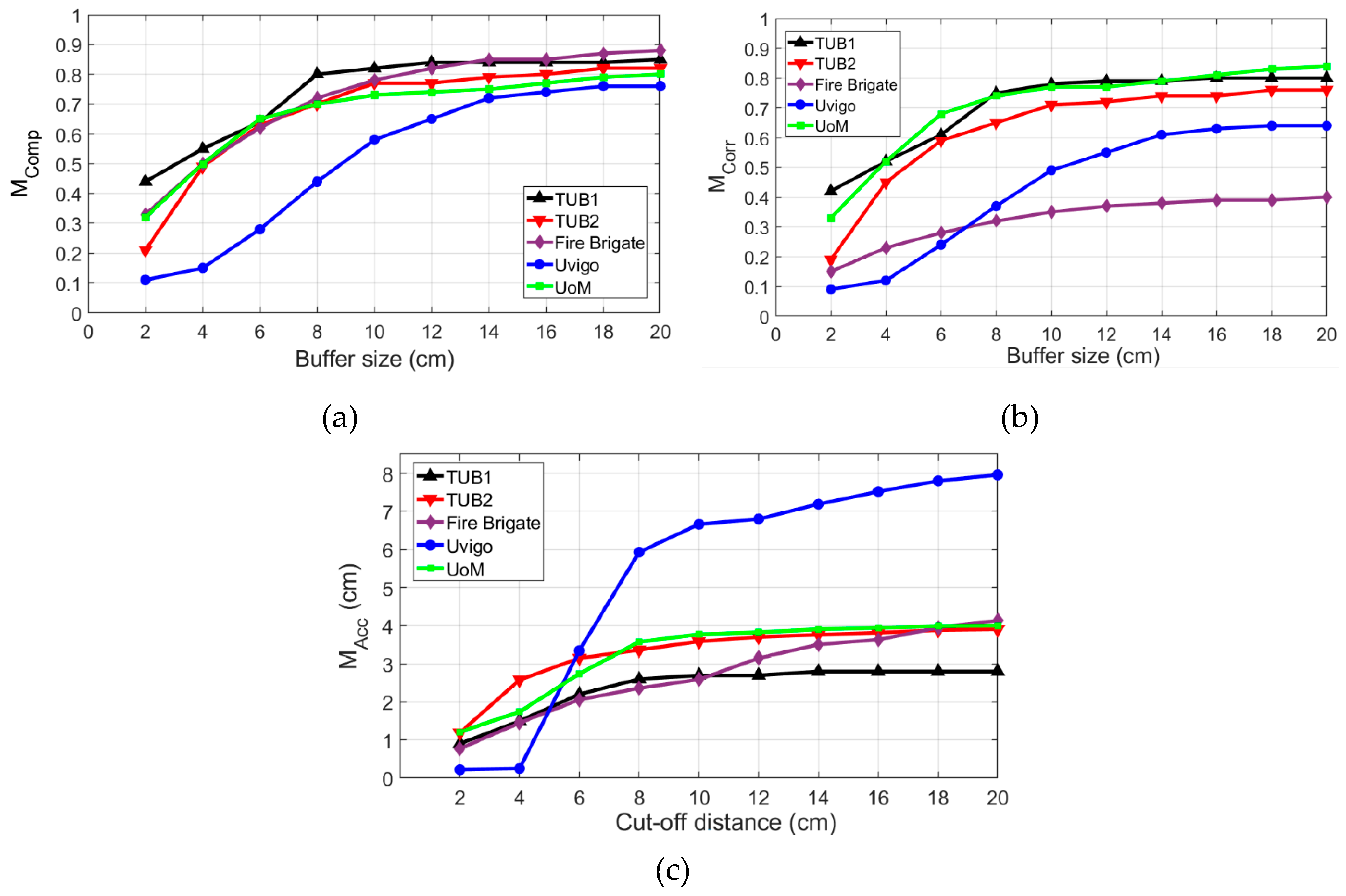
In order to gain insight into the quality of the reconstructed models, we compare the models with the corresponding ground truth models provided in the ISPRS Benchmark data sets [45]. The evaluation is based on the comparison of wall surfaces bounding the interior spaces of the reconstructed models with visible wall surfaces of the ground truths in terms of completeness, correctness, and accuracy using the evaluation approach proposed by Tran et al. [3]. Figure 20 shows the quality curves of the five reconstructed models of TUB1, the 2nd floor of TUB2, Fire Brigade, UVigo, and UoM. In general, the reconstructed models have relatively high completeness ( at ). While the walls in the three models TUB1, TUB2, and UoM achieve relatively high correctness ( at ), the Fire Brigade model contains a considerable amount of incorrect wall surfaces ( at ). The models TUB1, TUB2, Fire Brigade, and UoM achieve quite high levels of accuracy ( at ), and the reconstructed model of UVigo has lower accuracy (). These accuracies inherently represent the accuracy of locations of building surfaces in the reconstructed models. A comparison with other approaches submitted to the ISPRS Benchmark on Indoor Modelling [45] shows that the proposed approach achieves higher correctness for all the reconstructed models and higher completeness for three of the data sets (i.e., TUB2, Fire Brigade, and UVigo) but similar accuracy for four of the data sets (i.e., TUB1, TUB2, Fire Brigade, and UoM) [46]. Meanwhile, the accuracy of the reconstructed model for the UVigo data set is slightly lower.
6. Conclusions and Future Work
In this paper, a method for procedural reconstruction of 3D indoor models from point clouds is presented. The method is based on the combination of a shape grammar and a data-driven process using the rjMCMC algorithm. The integration facilitates the automated application of grammar rules. Consequently, it provides flexibility in modelling different building architectures, including Manhattan and non-Manhattan World designs. Additionally, the integration between the local characteristic of data and the model plausibility as well as taking into account the current state of the model enhances the robustness of the method to incompleteness and inaccuracy data. Experiments with several point clouds of synthetic and real indoor environments demonstrated the potential of the proposed approach for generating indoor models with high geometric accuracy and rich semantics as well as topological relations from lidar data with a high level of clutter.
The current indoor grammar is limited to buildings with planar surfaces. The doors are also manually added to the model by simply updating the containment attribute of walls without reconstructing their geometry. In the future, we will investigate the extension of the indoor grammar to buildings with nonplanar elements (e.g., beams and curved walls). We will also investigate the extension of the proposed shape grammar to allow geometric reconstruction of details such as door, windows, and stairs. A method for efficient extraction of structural surfaces of large and complex buildings is also a future work of this research.
Author Contributions
Conceptualization, H.T. and K.K.; methodology, H.T. and K.K.; software, H.T.; validation, H.T.; formal analysis, H.T.; investigation, H.T.; resources, K.K.; data curation, H.T.; writing-original draft preparation, H.T.; writing-review and editing, H.T. and K.K.; visualization, H.T. and K.K.; supervision, K.K.. All authors have read and agreed to the published version of the manuscript.
Funding
This research received no external funding
Acknowledgments
The first author acknowledges the financial support from the University of Melbourne through Melbourne International Fee Remission and Melbourne International Research Scholarship.
Conflicts of Interest
The authors declare no conflict of interest.
References
- Pătrăucean, V.; Armeni, I.; Nahangi, M.; Yeung, J.; Brilakis, I.; Haas, C. State of research in automatic as-built modelling. Adv. Eng. Inform. 2015, 29, 162–171. [Google Scholar] [CrossRef] [Green Version]
- Volk, R.; Stengel, J.; Schultmann, F. Building Information Modeling (BIM) for existing buildings—Literature review and future needs. Autom. Constr. 2014, 38, 109–127. [Google Scholar] [CrossRef] [Green Version]
- Tran, H.; Khoshelham, K.; Kealy, A. Geometric comparison and quality evaluation of 3D models of indoor environments. ISPRS J. Photogramm. Remote Sens. 2019, 149, 29–39. [Google Scholar] [CrossRef]
- Mura, C.; Mattausch, O.; Pajarola, R. Piecewise-planar Reconstruction of Multi-room Interiors with Arbitrary Wall Arrangements. In Computer Graphics Forum; Wiley Online Library: Hoboken, NJ, USA, 2016; pp. 179–188. [Google Scholar]
- Oesau, S.; Lafarge, F.; Alliez, P. Indoor scene reconstruction using feature sensitive primitive extraction and graph-cut. ISPRS J. Photogramm. Remote Sens. 2014, 90, 68–82. [Google Scholar] [CrossRef] [Green Version]
- Previtali, M.; Scaioni, M.; Barazzetti, L.; Brumana, R. A flexible methodology for outdoor/indoor building reconstruction from occluded point clouds. ISPRS Ann. Photogramm. Remote Sens. Spat. Inf. Sci. 2014, 2, 119. [Google Scholar] [CrossRef] [Green Version]
- Thomson, C.; Boehm, J. Automatic geometry generation from point clouds for BIM. Remote Sens. 2015, 7, 11753–11775. [Google Scholar] [CrossRef] [Green Version]
- Tran, H.; Khoshelhama, K. A stochastic approach to automated reconstruction of 3D models of interior spaces from point clouds. ISPRS Ann. Photogramm. Remote Sens. Spat. Inf. Sci. 2019, 299–306. [Google Scholar] [CrossRef] [Green Version]
- Gröger, G.; Plümer, L. Derivation of 3D indoor models by grammars for route planning. Photogramm. Fernerkund. Geoinf. 2010, 2010, 191–206. [Google Scholar]
- Khoshelham, K.; Díaz-Vilariño, L. 3D modelling of interior spaces: Learning the language of indoor architecture. Int. Arch. Photogramm. Remote Sens. Spat. Inf. Sci. 2014, 40, 321. [Google Scholar] [CrossRef] [Green Version]
- Tran, H.; Khoshelham, K.; Kealy, A.; Díaz-Vilariño, L. Shape Grammar Approach to 3D Modeling of Indoor Environments Using Point Clouds. J. Comput. Civ. Eng. 2019, 33, 04018055. [Google Scholar] [CrossRef]
- Becker, S. Generation and application of rules for quality dependent façade reconstruction. ISPRS J. Photogramm. Remote Sens. 2009, 64, 640–653. [Google Scholar] [CrossRef]
- Müller, P.; Wonka, P.; Haegler, S.; Ulmer, A.; Van Gool, L. Procedural modeling of buildings. In ACM SIGGRAPH; ACM: New York, NY, USA, 2006; pp. 614–623. [Google Scholar]
- Wonka, P.; Wimmer, M.; Sillion, F.; Ribarsky, W. Instant architecture. ACM Trans. Graph. (Tog) 2003, 22, 669–677. [Google Scholar] [CrossRef]
- Becker, S.; Peter, M.; Fritsch, D. Grammar-Supported 3D Indoor Reconstruction from Point Clouds for “AS-BUILT” BIM. ISPRS Ann. Photogramm. Remote Sens. Spat. Inf. Sci. 2015, 2. [Google Scholar] [CrossRef] [Green Version]
- Metropolis, N.; Rosenbluth, A.W.; Rosenbluth, M.N.; Teller, A.H.; Teller, E. Equation of state calculations by fast computing machines. J. Chem. Phys. 1953, 21, 1087–1092. [Google Scholar] [CrossRef] [Green Version]
- Dick, A.R.; Torr, P.H.; Cipolla, R. Modelling and interpretation of architecture from several images. Int. J. Comput. Vis. 2004, 60, 111–134. [Google Scholar] [CrossRef] [Green Version]
- Ripperda, N.; Brenner, C. Application of a formal grammar to facade reconstruction in semiautomatic and automatic environments. In Proceedings of the 12th AGILE Conference on GIScience, Berlin, Germany, 2–5 June 2009; Springer: Berlin, Germany, 2009; pp. 103–157. [Google Scholar]
- Elberink, S.O.; Khoshelham, K. Automatic extraction of railroad centerlines from mobile laser scanning data. Remote Sens. 2015, 7, 5565–5583. [Google Scholar] [CrossRef] [Green Version]
- Schmidt, A.; Lafarge, F.; Brenner, C.; Rottensteiner, F.; Heipke, C. Forest point processes for the automatic extraction of networks in raster data. ISPRS J. Photogramm. Remote Sens. 2017, 126, 38–55. [Google Scholar] [CrossRef] [Green Version]
- Merrell, P.; Schkufza, E.; Koltun, V. Computer-generated residential building layouts. In ACM SIGGRAPH Asia 2010 Papers; ACM: New York, NY, USA, 2010; pp. 1–12. [Google Scholar]
- Adan, A.; Huber, D. 3D reconstruction of interior wall surfaces under occlusion and clutter. In Proceedings of the 2011 International Conference on 3D Imaging, Modeling, Processing, Visualization and Transmission, Hangzhou, China, 16–19 May 2011; pp. 275–281. [Google Scholar]
- Díaz-Vilariño, L.; Khoshelham, K.; Martínez-Sánchez, J.; Arias, P. 3D modeling of building indoor spaces and closed doors from imagery and point clouds. Sensors 2015, 15, 3491–3512. [Google Scholar] [CrossRef] [Green Version]
- Hong, S.; Jung, J.; Kim, S.; Cho, H.; Lee, J.; Heo, J. Semi-automated approach to indoor mapping for 3D as-built building information modeling. Comput. Environ. Urban Syst. 2015, 51, 34–46. [Google Scholar] [CrossRef]
- Sanchez, V.; Zakhor, A. Planar 3D modeling of building interiors from point cloud data. In Proceedings of the 2012 19th IEEE International Conference on Image Processing, Orlando, FL, USA, 30 September–3 October 2012; pp. 1777–1780. [Google Scholar]
- Xiong, X.; Adan, A.; Akinci, B.; Huber, D. Automatic creation of semantically rich 3D building models from laser scanner data. Autom. Constr. 2013, 31, 325–337. [Google Scholar] [CrossRef] [Green Version]
- Macher, H.; Landes, T.; Grussenmeyer, P. From point clouds to building information models: 3D semi-automatic reconstruction of indoors of existing buildings. Appl. Sci. 2017, 7, 1030. [Google Scholar] [CrossRef] [Green Version]
- Nikoohemat, S.; Diakité, A.A.; Zlatanova, S.; Vosselman, G. Indoor 3D reconstruction from point clouds for optimal routing in complex buildings to support disaster management. Autom. Constr. 2020, 113, 103109. [Google Scholar] [CrossRef]
- Previtali, M.; Díaz-Vilariño, L.; Scaioni, M. Indoor building reconstruction from occluded point clouds using graph-cut and ray-tracing. Appl. Sci. 2018, 8, 1529. [Google Scholar] [CrossRef] [Green Version]
- Ochmann, S.; Vock, R.; Wessel, R.; Klein, R. Automatic reconstruction of parametric building models from indoor point clouds. Comput. Graph. 2016, 54, 94–103. [Google Scholar] [CrossRef] [Green Version]
- Ochmann, S.; Vock, R.; Klein, R. Automatic reconstruction of fully volumetric 3D building models from oriented point clouds. ISPRS J. Photogramm. Remote Sens. 2019, 151, 251–262. [Google Scholar] [CrossRef] [Green Version]
- Marvie, J.-E.; Perret, J.; Bouatouch, K. The FL-system: A functional L-system for procedural geometric modeling. Vis. Comput. 2005, 21, 329–339. [Google Scholar] [CrossRef]
- Mitchell, W.J. The Logic of Architecture: Design, Computation, and Cognition; MIT Press: Cambridge, MA, USA, 1990. [Google Scholar]
- Parish, Y.I.; Müller, P. Procedural modeling of cities. In Proceedings of the 28th Annual Conference on Computer Graphics and Interactive Techniques, Los Angeles, CA, USA, 12–17 August 2001; pp. 301–308. [Google Scholar]
- Stiny, G.; Gips, J. Shape grammars and the generative specification of painting and sculpture. In Proceedings of the IFIP Congress (2), Amsterdam, The Netherlands, 23–28 August 1971; pp. 125–135. [Google Scholar]
- Schnabel, R.; Wahl, R.; Klein, R. Efficient RANSAC for point-cloud shape detection. In Computer Graphics Forum; Wiley Online Library: Hoboken, NJ, USA, 2007. [Google Scholar]
- Khoshelham, K. Closed-form solutions for estimating a rigid motion from plane correspondences extracted from point clouds. ISPRS J. Photogramm. Remote Sens. 2016, 114, 78–91. [Google Scholar] [CrossRef]
- Agarwal, P.K.; Sharir, M. Arrangements and their applications. In Handbook of Computational Geometry; Elsevier: Amsterdam, The Netherlands, 2000; pp. 49–119. [Google Scholar]
- CGAL. Computational Geometry Algorithms Library. 2019. Available online: http://www.cgal.org (accessed on 15 January 2020).
- Stiny, G. Shape: Talking about Seeing and Doing; MIt Press: Cambridge, MA, USA, 2006. [Google Scholar]
- Hastings, W.K. Monte Carlo sampling methods using Markov chains and their applications. Biometrika 1970, 57, 97–109. [Google Scholar] [CrossRef]
- Tran, H.; Khoshelham, K. Building Change Detection through Comparison of a Lidar Scan with a Building Information Model. Int. Arch. Photogramm. Remote Sens. Spat. Inf. Sci. 2019. [Google Scholar] [CrossRef] [Green Version]
- Edelsbrunner, H.; Mücke, E.P. Three-dimensional alpha shapes. ACM Trans. Graph. 1994, 13, 43–72. [Google Scholar] [CrossRef]
- Rissanen, J. A Universal Prior for Integers and Estimation by Minimum Description Length. Ann. Stat. 1983, 11, 416–431. [Google Scholar] [CrossRef]
- Khoshelham, K.; Vilariño, L.D.; Peter, M.; Kang, Z.; Acharya, D. The ISPRS benchmark on indoor modelling. Int. Arch. Photogramm. Remote Sens. Spat. Inf. Sci 2017, 42, 367–372. [Google Scholar] [CrossRef] [Green Version]
- ISPRS Initiative, ISPRS Benchmark on Indoor Modelling. 2020. Available online: http://www2.isprs.org/commissions/comm4/wg5/benchmark-test-on-indoor-modelling.html (accessed on 15 January 2020).
Figure 1.
Overview of the proposed approach.

Figure 2.
Point clustering: (a) an input point cloud of a hexagonal building; (b) vertical points; (c) horizontal points; and (d) other points (e.g., clutter and noise).
Figure 2.
Point clustering: (a) an input point cloud of a hexagonal building; (b) vertical points; (c) horizontal points; and (d) other points (e.g., clutter and noise).

Figure 3.
Local-scale surface extraction: (a) voxelized structure of the input point cloud; (b) extracted vertical surfaces; and (c) extracted horizontal surfaces.
Figure 3.
Local-scale surface extraction: (a) voxelized structure of the input point cloud; (b) extracted vertical surfaces; and (c) extracted horizontal surfaces.

Figure 4.
Globally refined surfaces of the hexagon building: (a) vertical surfaces and (b) horizontal surfaces.
Figure 4.
Globally refined surfaces of the hexagon building: (a) vertical surfaces and (b) horizontal surfaces.

Figure 5.
Three-dimensional cell decomposition: (a) horizontal and vertical surfaces; (b) 2D cell decomposition of a horizontal structure (i.e., floor); and (c) 3D cell decomposition.
Figure 5.
Three-dimensional cell decomposition: (a) horizontal and vertical surfaces; (b) 2D cell decomposition of a horizontal structure (i.e., floor); and (c) 3D cell decomposition.

Figure 6.
Geometric representation of a 3D shape and its scope.

Figure 7.
Reversible merging and splitting: Merging: from left to right, the two adjacent spaces and are merged to form space B. Splitting: from right to left, shape B is split into its two component shapes and .
Figure 7.
Reversible merging and splitting: Merging: from left to right, the two adjacent spaces and are merged to form space B. Splitting: from right to left, shape B is split into its two component shapes and .

Figure 8.
Reversible classification-declassification processes. Classification: from left to right by labelling a shape as an interior space (green). Declassification: from right to left by nulling the label of the interior space.
Figure 8.
Reversible classification-declassification processes. Classification: from left to right by labelling a shape as an interior space (green). Declassification: from right to left by nulling the label of the interior space.

Figure 9.
An example of topological relations between two nonterminal interior spaces and (a), which are in an adjacency relation represented by the red dotted line (b) and in a connectivity relation represented by the black solid line (c), as there is no actual surface between them.
Figure 9.
An example of topological relations between two nonterminal interior spaces and (a), which are in an adjacency relation represented by the red dotted line (b) and in a connectivity relation represented by the black solid line (c), as there is no actual surface between them.

Figure 10.
An example of containment relation (c) between the two interior spaces and (a) and their merged shape B (b).
Figure 10.
An example of containment relation (c) between the two interior spaces and (a) and their merged shape B (b).

Figure 11.
Production procedure: The small rectangles represent applications of grammar rules. The horizontal and vertical arrows indicate the sequence of the rule applications. The arrow on the top of a rule indicates iteration. The symbol I indicates the initial starting shape.
Figure 11.
Production procedure: The small rectangles represent applications of grammar rules. The horizontal and vertical arrows indicate the sequence of the rule applications. The arrow on the top of a rule indicates iteration. The symbol I indicates the initial starting shape.

Figure 12.
The synthetic data set, including a synthetic point cloud (left) and a ground truth model.
Figure 12.
The synthetic data set, including a synthetic point cloud (left) and a ground truth model.

Figure 13.
The real data sets including point clouds (left) and ground truth models (right): (a) the Office and (b) the Museum.
Figure 13.
The real data sets including point clouds (left) and ground truth models (right): (a) the Office and (b) the Museum.

Figure 14.
Reconstructed models, including the models’ 3D cell decomposition (left) and the final models (right): (a) SYN; (b) Office; and (c) Museum. Green surfaces represent interior spaces (i.e., rooms and corridors), and red surfaces represent volumetric walls.
Figure 14.
Reconstructed models, including the models’ 3D cell decomposition (left) and the final models (right): (a) SYN; (b) Office; and (c) Museum. Green surfaces represent interior spaces (i.e., rooms and corridors), and red surfaces represent volumetric walls.


Figure 15.
Quality evaluation of the final models in terms of completeness (a), correctness (b), and accuracy (c).
Figure 15.
Quality evaluation of the final models in terms of completeness (a), correctness (b), and accuracy (c).

Figure 16.
Localization of completeness and correctness errors of the Museum: (a) the completeness errors localized in the ground truth and (b) the correctness errors localized in the reconstructed model.
Figure 16.
Localization of completeness and correctness errors of the Museum: (a) the completeness errors localized in the ground truth and (b) the correctness errors localized in the reconstructed model.

Figure 17.
Topological graphs between interior spaces of the Museum: (a) adjacency and containment relations and (b) connectivity and containment relations.
Figure 17.
Topological graphs between interior spaces of the Museum: (a) adjacency and containment relations and (b) connectivity and containment relations.

Figure 18.
The connectivity relations (black solid line) between final spaces (i.e., rooms and corridors) of the Museum.
Figure 18.
The connectivity relations (black solid line) between final spaces (i.e., rooms and corridors) of the Museum.

Figure 19.
The ISPRS indoor modelling benchmark point clouds and the corresponding models reconstructed by the proposed approach: (a) TUB1; (b) TUB2; (c) Fire Brigade; (d) UVigo; and (e) UoM.
Figure 19.
The ISPRS indoor modelling benchmark point clouds and the corresponding models reconstructed by the proposed approach: (a) TUB1; (b) TUB2; (c) Fire Brigade; (d) UVigo; and (e) UoM.


Figure 20.
Quality evaluation of visible wall surfaces of the models reconstructed from the ISPRS Benchmark data sets in terms of completeness (a), correctness (b), and accuracy (c).
Figure 20.
Quality evaluation of visible wall surfaces of the models reconstructed from the ISPRS Benchmark data sets in terms of completeness (a), correctness (b), and accuracy (c).


Table 1.
Overview of reconstructed features by recent indoor modelling approaches.
| Ref. (Year) | Non-Manhattan | Volumetric walls | Volumetric spaces | Topological relations |
|---|---|---|---|---|
| [4] Mura et al. (2016) | Yes | No | No | No |
| [5] Oesau et al. (2014) | Yes | No | No | No |
| [9] Gröger and Plümer (2010) | No | No | Yes | Yes |
| [10] Khoshelham and Díaz-Vilariño (2014) | No | No | Yes | No |
| [11] Tran et al. (2019) | No | Yes | Yes | Yes |
| [15] Becker et al. (2015) | No | Yes | No | No |
| [26] Xiong et al. (2013) | No | No | No | No |
| [27] Macher et al. (2017) | No | Yes | No | No |
| [28] Nikoohemat et al. (2020) | Yes | Yes | Yes | No |
| [30] Ochmann et al. (2016) | Yes | Yes | No | No |
| [31] Ochmann et al. (2019) | Yes | Yes | No | No |
| Ours | Yes | Yes | Yes | Yes |
Table 2.
Parameter settings used in the experiments.
| Parameters Data Set | Max wall Thickness (m) | Voxel Size (m) | Convergence Factor | Normalization Factors | |||||
|---|---|---|---|---|---|---|---|---|---|
| Case 1 | Case 2 | Case 3 | |||||||
| SYN | 0.3 | 5.0 | 0.0 | 1/3 | 1/3 | 1/3 | 1.0 | 0.8 | 0.9 |
| Office | 0.3 | 3.0 | 0.2 | 1/3 | 1/3 | 1/3 | 1.0 | 0.8 | 0.9 |
| Museum | 0.4 | 3.0 | 0.1 | 1/3 | 1/3 | 1/3 | 1.0 | 0.8 | 0.9 |
© 2020 by the authors. Licensee MDPI, Basel, Switzerland. This article is an open access article distributed under the terms and conditions of the Creative Commons Attribution (CC BY) license (http://creativecommons.org/licenses/by/4.0/).
Share and Cite
MDPI and ACS Style
Tran, H.; Khoshelham, K. Procedural Reconstruction of 3D Indoor Models from Lidar Data Using Reversible Jump Markov Chain Monte Carlo. Remote Sens. 2020, 12, 838. https://doi.org/10.3390/rs12050838
AMA Style
Tran H, Khoshelham K. Procedural Reconstruction of 3D Indoor Models from Lidar Data Using Reversible Jump Markov Chain Monte Carlo. Remote Sensing. 2020; 12(5):838. https://doi.org/10.3390/rs12050838
Chicago/Turabian StyleTran, Ha, and Kourosh Khoshelham. 2020. "Procedural Reconstruction of 3D Indoor Models from Lidar Data Using Reversible Jump Markov Chain Monte Carlo" Remote Sensing 12, no. 5: 838. https://doi.org/10.3390/rs12050838
Note that from the first issue of 2016, this journal uses article numbers instead of page numbers. See further details here.