Article

Machine Learning Algorithms to Predict Forage Nutritive Value of In Situ Perennial Ryegrass Plants Using Hyperspectral Canopy Reflectance Data

1
School of Applied Systems Biology, La Trobe University, Bundoora, VIC 3086, Australia
2
Agriculture Victoria, Hamilton Centre, Hamilton, VIC 3300, Australia
3
Agriculture Victoria, Ellinbank Centre, 1301 Hazeldean Road, Ellinbank, VIC 3821, Australia
4
Agriculture Victoria, AgriBio, Centre for AgriBioscience, Bundoora, VIC 3083, Australia
5
Faculty of Veterinary and Agricultural Sciences, The University of Melbourne, Melbourne, VIC 3010, Australia
*
Author to whom correspondence should be addressed.
Remote Sens. 2020, 12(6), 928; https://doi.org/10.3390/rs12060928
Submission received: 27 January 2020 / Revised: 10 March 2020 / Accepted: 10 March 2020 / Published: 13 March 2020
(This article belongs to the Section Remote Sensing in Agriculture and Vegetation)

Abstract

:
Nutritive value (NV) of forage is too time consuming and expensive to measure routinely in targeted breeding programs. Non-destructive spectroscopy has the potential to quickly and cheaply measure NV but requires an intermediate modelling step to interpret the spectral data. A novel machine learning technique for forage analysis, Cubist, was used to analyse canopy spectra to predict seven NV parameters, including dry matter (DM), acid detergent fibre (ADF), ash, neutral detergent fibre (NDF), in vivo dry matter digestibility (IVDMD), water soluble carbohydrates (WSC), and crude protein (CP). Perennial ryegrass (Lolium perenne) was used as the test crop. Independent validation of the developed models revealed prediction capabilities with R2 values and Lin’s concordance values reported between 0.49 and 0.82, and 0.68 and 0.89, respectively. Informative wavelengths for the creation of predictive models were identified for the seven NV parameters. These wavelengths included regions of the electromagnetic spectrum that are usually excluded due to high background variation, however, they contain important information and utilising them to obtain meaningful signals within the background variation is an advantage for accurate models. Non-destructive field spectroscopy along with the predictive models was deployed infield to measure NV of individual ryegrass plants. A significant reduction in labour was observed. The associated increase in speed and reduction of cost makes targeting NV in commercial breeding programs now feasible.

Graphical Abstract

1. Introduction

Using hyperspectral sensors in crop research is increasingly common for complex traits that multispectral sensors have failed to describe, because these sensors capture a large amount of information without the need for destructive harvesting [1,2] Non-destructive measurement removes many time consuming and costly steps from data capture and analysis. As a result, it makes an appealing option for phenotyping, particularly for quantitative traits, the improvement of which requires selection from large sample numbers with traditional plant breeding [3]. One such trait is nutritive value (NV) of forage, which is economically important to the dairy and red meat industry in Australia [4]. Improving the NV of forage would be beneficial to primary producers with grazing stock as it would increase the carrying capacity of paddocks [5]. The NV of forage is the culmination of multiple parameters that all contribute to the amount of energy and nutrition derived by digestion. Development of high NV cultivars requires a method of monitoring the expression of NV parameters in the field 2001, which is necessary as glasshouse trials are often poorly correlated with results in field grown plants [6].
It is imperative to measure the phenotypes across different environmental conditions as the expression of NV characteristics in forage grasses are heavily influenced by various abiotic and biotic conditions such as soil type and water availability [7,8]. The growth stage of the plant also affects NV 2017, with a notable decline in positive forage traits such as in vivo dry matter digestibility (IVDMD) and increase in negative traits such as neutral detergent fibre (NDF) when the grass enters its reproductive phase [8]. The inherent variability of forage, both within the genome of the species and across seasons necessitates high volumes of data capture and analysis to improve forage NV. Unfortunately, 1999, this variability also makes measuring NV in the field more challenging than more uniform crops like wheat and maize. Hyperspectral sensors may be a solution to measuring in large outdoor trials in situ since they can be used to gather large amounts of phenotypic data rapidly [2,6].
The industry standard method for determining NV in forages is the use of Near Infrared (NIR) spectroscopy conducted in laboratory conditions using dried, ground herbage samples, which are calibrated and validated by wet chemistry [9]. Though this method is accurate and reliable it does constrain sample numbers due to the cost and time involved in analysis [10]. Transitioning to field-based 2005, non-destructive spectroscopy would drastically decrease the time and cost involved in analysis of NV, making it possible to directly target NV traits in breeding programs [11,12,13]. Unfortunately, field spectroscopy captures significant environmental signals that are not related to the target trait, but are due to solar radiation, light levels, recent precipitation events, and plant structure, making it challenging to retrieve biophysical parameters from background variation [14,15]. The important signals may be weak and hidden within many overlapping peaks and troughs [16]. Additionally, relationships between biophysical parameters and spectra are often nonlinear and are difficult to identify with linear models [17]. Various spectral pre-processing approaches have been used to reduce background variation in the spectra and increase the relevant signals from biochemical parameters [18]. Pre-treatments may correct baseline drift 2019, or correct the effect of overlapping peaks, and improve the simplicity and robustness of the calibration [19].
Creating an empirical model with spectral data always involves an intermediate modelling step [14]. One option is to create non-parametric models 2011, which use a training set of spectral data and corresponding laboratory results [18]. Non-parametric algorithms such as principal component analysis (PCA), or partial least square regression (PLSR) are often employed to retrieve biophysical parameters of vegetation from spectra [20,21]. In many cases the combination of spectral pre-processing techniques and model building techniques that works best varies from one parameter to the next [22]. Finding the best combination of spectral pre-treatment and regression model for each parameter often involves trialing combinations and examining the predictive statistics 2010, after which models that perform well should be tested with independent data [15,23]. The accuracy of predictive models created with spectra tends to be limited spatially and temporally to the training data sets that create them. Testing models with independent data is important for creating robust models and being able to discern NV parameters of plants from different growth stages and ecotypes [24].
Data mining and machine learning approaches have been successfully used to create predictive models with the large data sets associated with crop research [25]. An example of a data mining method is tree-based regression 2018, which is often utilised for continuous class data such as spectral data [26]. An example of machine learning is Support Vector Machine (SVM), a modelling approach that uses a supervised learning algorithm to find both linear and non-linear relationships in data [27]. SVM has been used to predict nitrogen uptake 1999, dry matter, and crude protein in grass and clover forage with R2 between 0.90 and 0.98 [17]. Another commonly used machine learning algorithm is Random Forest Regression, which creates thousands of regression trees and averages all the outputs for the prediction of dependent variables [20]. This technique has been applied to predict NDF 2019, acid detergent fibre (ADF), and lignin in tropical forage grasses [20].
Cubist is an alternative machine learning technique that is based on decision trees, with data partitioned into units of similar spectral signals and attributes with a hierarchy of rules determining the partitions [28]. Decision trees work well for simple discrete classification but less well for continuous measures. To address this problem Cubist uses decision trees that instead of ending in a binary decision 2011, end in a regression equation [28,29]. The rules have the formula of a boolean statement, an action for when true, and an alternative action for not true, (if[], then[], else[]). These rules divide data into similar classes which can then be more easily analysed with linear regression [29]. Cubist has been demonstrated to be an accurate alternative to PLSR and is ideal to be used for analysis of hyperspectral datasets [30]. Cubist models have been successfully utilised in other disciplines of agriculture and soil sciences; however, Cubist has not been tried as an approach for predicting NV values in forage plants from a field-based breeding nursery [30,31]. Cubist models are also able to provide the wavelengths utilised and a percentage of usefulness to prediction which makes this technique less of a “Blackbox” approach than other machine learning modelling options.
The aims of this study were to: (i) Use data mining techniques to extract biophysical parameters of perennial ryegrass from hyperspectral canopy data; (ii) Identify specific wavelengths important for modelling NV parameters in perennial ryegrass; (iii) Evaluate the predictive ability of Cubist models to analyse NV parameters with an independent dataset; (iv) Assess advantages of the machine learning approach for data analysis as well as potential limiting factors; (v) Demonstrate the use of the developed predictive models to analyse NV parameters from the canopy spectra of a large study population of 2880 plants.

2. Materials and Methods
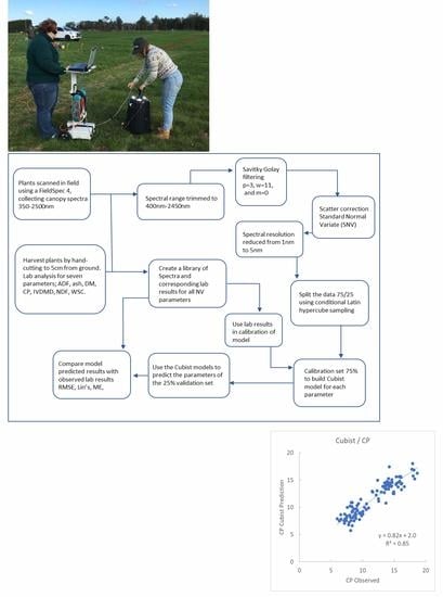
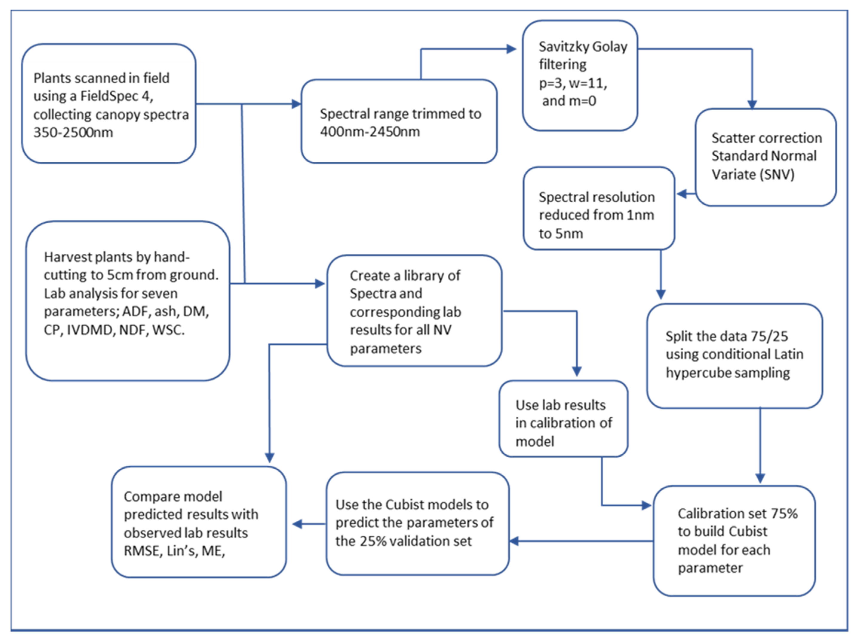
2.1. Study Site

All samples used in this study are from a perennial ryegrass field trial in Hamilton Victoria 2019, Australia (37.819440 S, 142.062171E. Fifty experimental varieties of perennial ryegrass were grown as plots of 96 individual ryegrass plants, with ten replicates of each plot. Spectral measurements from 960 of these plants were collected at four harvest dates over the course of the growing season of At each harvest a subset of 128 plants were cut immediately after scanning, then dried at 60°C for 48 h, then ground using a 1 mm grate for laboratory based NIR analysis. Seven nutritive value (NV) parameters were analysed using a Foss XDS analyser® including Ash 2019, crude protein (CP), in vivo dry matter digestibility (IVDMD), neutral detergent fibre (NDF), acid detergent fibre (ADF), water-soluble carbohydrates (WSC), and dry matter percentage (DM. Sixty-five plants were discarded from analysis as they had died between measurements or were too low in biomass for lab-analysis. A set of 156 data points from previous harvests of the trial were included to expand the calibration, making a total of 605 plants. Convex hull and Mahalanobis distance were then used to identify spectral outliers which were removed from the analysis if the H value was over 0.6, with sixty-five samples excluded [32]. In total, 540 samples with both lab results and spectra were used in this experiment to build and test the NV predictive models. The seven NV parameters were then predicted using scanned spectra obtained from 2880 samples (960 plants measured four times over the growing season.

2.2. Spectra Collection

The canopy spectra of 960 plants were collected at each harvest date using an ADS® FieldSpec Hi-Res 4 (Boulder 2019, CO, USA) with a 10° lens and scrambler. Spectra within the visual-NIR (350 nm to 2500 nm) range was recorded (Figure 1). For each sample, the spectra were measured 50 times and averaged. The spectrometer was calibrated after measuring each plot of 96 plants, approximately every 20 min. A light shield was used to reduce background spectral signals from the environment. The shield consisted of a 56 cm tall cylindrical plastic bin with a diameter of 45 cm, painted inside with matte black paint (Black 2.0©), and fitted with three tungsten halogen lights with spectral range of 300–2500 nm [22]. The light shield was equipped with a sensor holder that insured the sensor was always perpendicular to the ground and at 56 cm from the sample, creating a field of view of 79 cm2. A full description of the light shield is provided in Smith et al. 2019. The light shield and halogen lights were used instead of sunlight as a source of irradiance as this method was shown to be more successful for creating predictive models [21,22].

2.3. Spectra Data Pre-Processing

The software used for the pre-processing and model development was R version 3.5.3, reflectance spectra was trimmed, leaving between 400 nm to 2450 nm, this was done to remove the regions at the ends of the sensor range which contain a lot of background variation. The spectra were then filtered to every 5th wavelength, this decision was a balance between reducing the dimensionality of the data to prevent overfitting and retaining high spectral resolution so that important information is not lost, as hyperspectral reflectance data is highly autocorrelated and spectral variance captured at 1 nm resolution should still be present at 5 nm. To optimise the signal to noise ratio, Savitzky Golay smoothing was applied, with an interval width of 11 nm [33]. To reduce the impact of light scattering, a spectral scatter correction technique, standard normal variate (SNV) was used to scale each spectrum based on their standard deviation and mean [32].

2.4. Splitting Data as Model Calibration and Validation

R version 3.5.3 was also use for the data splitting; Conditional Latin hypercube sampling was used to split the samples with corresponding lab results into a calibration set of 75% and a validation set of 25% [32]. The calibration set included 405 samples and the validation set included 135 samples. A processing example of the cubist model is available upon request to the first author.

2.5. Spectral Model Development

Models were developed with Cubist algorithms using pre-processed spectra from the 405 calibration samples (Figure 2).

2.6. Model Validation

The model predictions and observed lab results were compared and several validation indices were derived to determine model performance, including mean square error (MSE) which depicts the model bias, root mean square error (RMSE) which depicts the model accuracy, Lin’s concordance correlation coefficient (LCC), and the correlation coefficient or R2 [34].

2.7. Model Prediction of Nutritive Value (NV)

Once the model prediction ability had been assessed, the best models were then used to predict the NV parameters in all plants which had been scanned for canopy reflectance (2880.

2.8. Model Variable Usage and Importance

Cubist provides wavelength usage statistics which gives the percentage of times a wavelength was used either in a condition or in a linear model [28]. The usage includes wavelengths used in predictive models created at each split of the tree and therefore also includes each variable used in the current split or any split above it [28].

2.9. Cubist Model Comparison to Partial Least Square Regression (PLSR) Model

In order to assess the advantages of the machine learning approach for data analysis 2012, the process was compared to a previously validated traditional approach, partial least square regression (PLSR. We have previously explored the use of non-destructive spectroscopy to assess NV in forage using PLSR as the intermediate modelling step. This previous study had very similar methodology, except the sample size was much smaller and the predictive models were developed with PLSR using the software WinISI®. To compare the predictive ability of cubist to PLSR, spectra of the total 109 samples used in the earlier study were run through the cubist models to predict seven NV parameters. As the earlier PLSR models were developed with much lower sample numbers, to make comparison fairer the PLSR models were redeveloped using the same calibration set of 405 sample used for the cubist models. The results given by the cubist models and the PLSR models were then compared to lab results of the 109 samples.

3. Results

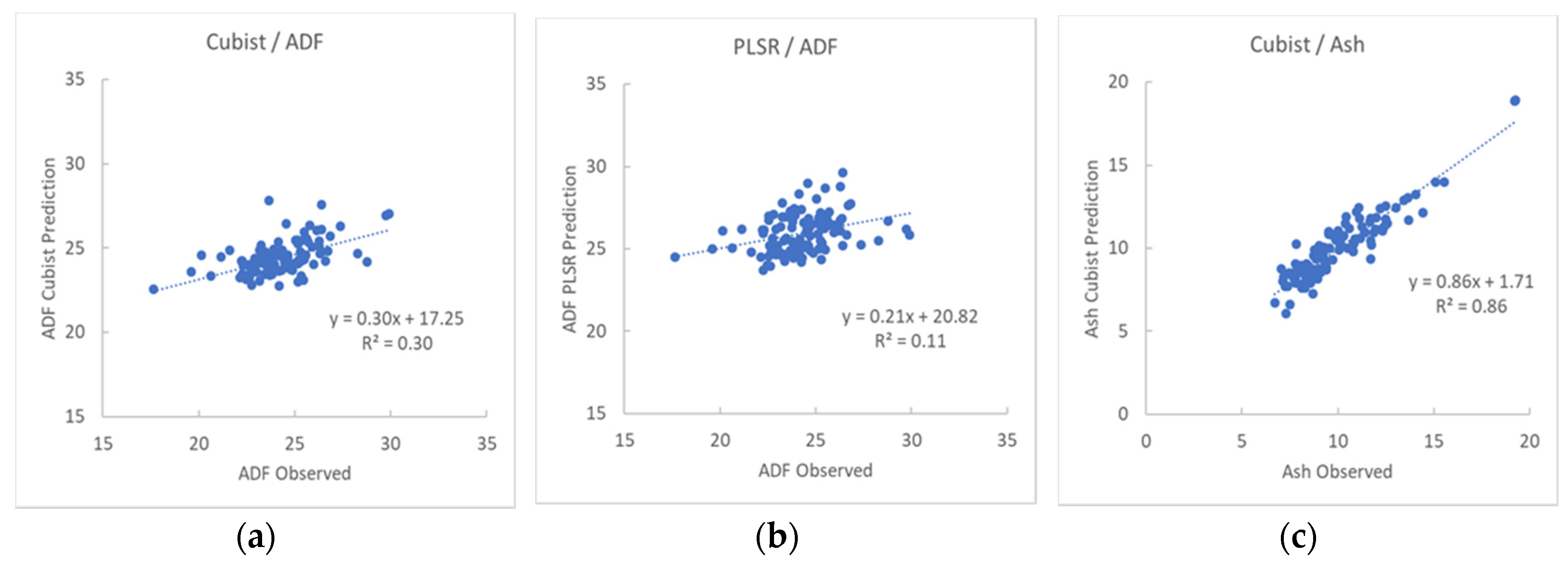
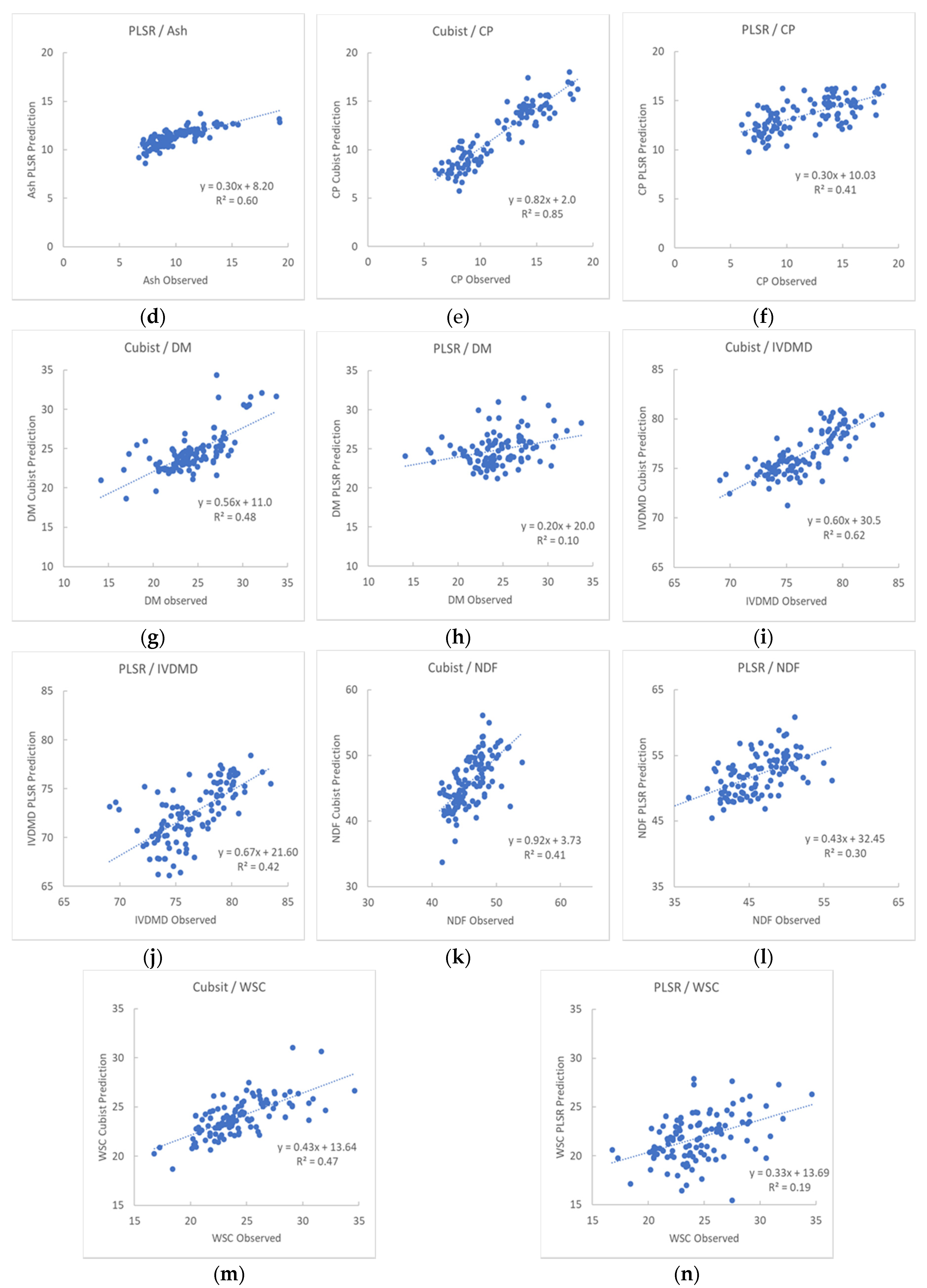
3.1. Descriptive Statistics and Evaluation of Model Performances for Key Nutritive Traits

After accumulating a library of spectra and corresponding lab results, Cubist models for the seven NV parameters ADF, ash, NDF, CP, IVDMD, WSC, and DM were created. Models for the all parameters showed decent predictive ability with R2 between 0.60 and 0.82, and LCC between 0.73 and 0.89 for the calibration results (Table 1), and for the independent validation R2 between 0.66 and 0.82, LCC between 0.82 and 0.89. The WSC model showed the lowest predictive ability with R2 of 0.49 and LCC of 0.68 (Table 1). The variability of NV parameters found in the samples used to build and validate the models are shown below in Table 2. The average, minimum, and maximum values of predicted NV results was slightly broader, showing that the models were able to extrapolate (Table 2). The spectra of perennial ryegrass are highly variable, this variation comes from many sources, as each plant will have differences in leaf structure, water content, and other biophysical parameters all of which contribute to the spectral signature [35]. The changing environmental conditions over the growing season also increase the spectral variability. Though the spectra are highly variable 2017, the NV parameters do not have a wide range of values (Table 2). This illustrates the challenges of finding spectral response to biophysical parameters, as they are often less prominent than signals relating to the environmental components and the three-dimensional structure of the plant.
The statistics given are, including mean square error (MSE) which depicts the model bias, root mean square error (RMSE) which depicts the model accuracy, Lin’s concordance correlation coefficient (LCC), and the correlation coefficient or (R2. Parameters listed are (ADF), ash, dry matter (DM), crude protein (CP), in vivo dry matter digestibility (IVDMD), neutral detergent fibre (NDF), and water-soluble carbohydrates (WSC.)

3.2. Application of Models for High-Throughput NV Prediction

To compare difference in time taken to analyse a single sample between the lab-based approach and field-based approach required calculating the average time a single sample would take with either method. The time required to analyse a plant sample with lab-based spectroscopy was calculated by combining the total time for identification and hand cutting plants, oven drying the samples at 60°C for 48 h, grinding the samples to a fine powder in a mechanical grinder with a 1mm grate, then scanning of all samples in a lab-based spectrometer. The total time taken to measure samples was then divided by the number of samples measured, averaging 15 min. The time required for analysis of a single plant with field-based spectroscopy was calculated by combining the time needed to identify plants, measure the reflectance spectra, and run the spectra through the predictive models. This time was then divided by the number of samples analysed averaging 30 s, making the field-based approach 30 times faster than the lab-based approach.

3.3. Key Model Drivers for Prediction

The Cubist models produce a list of variable importance, which is a combination of wavelength usage in the rule conditions for data splitting and wavelengths used in the regression [28]. The usage percentage of wavelengths for this study can be found in the additional information.

3.4. Cubist Model Comparison to PLSR Model

The predicted results from cubist models were compared to lab results 2012, the PLSR predicted results were also compared to lab results.
When comparing the predicted results of NV parameters determined using Cubist to lab results the models showed consistently stronger regressions than models created using PLSR with the same data set (Figure 3). The samples used in the above analysis were from the same field trial but measured in a previous year to all the samples that had been used in the model calibration, showing that the Cubist model is robust enough to cover multiple years of analysis.

4. Discussion

4.1. Data Mining Techniques to Extract Biophysical Parameters of Perennial Ryegrass

This study demonstrates that it is possible to predict NV parameters in large populations of perennial ryegrass grown in natural, outdoor conditions. The cubist models showed strong predictive statistics for all parameters with R2 between 0.49 and 0.82 and LCCs of between 0.68 and 0.89 for the validation of models with samples not included in their calibration (Table 1). The minimum, maximum and average value for each parameter were calculated for both the 540 samples with lab results in the calibration set and the 2880 predicted values (Table 2). The predictive models were able to cover the range of NV values included in the calibration but also extrapolate to predict higher or lower values if necessary.
As a pipeline for selection of high NV plants for breeding purposes, this system will be rapid and cost effective once the initial work of developing the models is complete, however, the initial cost of the equipment and lab-analysis of the calibration may still be prohibitively expensive. Portable spectrometers are comparatively expensive to lab-based systems and cover a similar range and resolution of wavelengths. The software used to analyse the spectra is open sourced.

4.2. Identify Specific Wavelengths Important for Modelling NV Parameters in Perennial Ryegrass

An advantage of Cubist model is that it provides the percentage of use for the wavelengths utilised by the model [30]. This identifies the most important wavelengths for each parameter and collectively for NV in ryegrass. The wavelengths selected were often from biophysically meaningful regions of the spectrum which is promising that the model will be robust for use in other field trials [36]. By routinely identifying wavelengths important to modelling NV 2013, the parsimonious wavelengths for each parameter can be identified. Identifying important wavelengths for each parameter, along with the percentage of usage could be used for further refinement of the models and for designing sensors with reduced range and resolution. For instance, this information can be used to develop a cheaper, lighter sensor that captures only the parsimonious wavelengths for forage NV. This would have the added advantage of reduced data dimensionality, removing unnecessary wavelengths to diminish the number of redundant variables in models [37]. Additionally, Cubist variable importance (percent usage) could potentially be used to develop customized multispectral cameras for capturing spectral images of samples in NV parsimonious wavelengths.
The key model drivers for prediction were varied and ranged across the entire electromagnetic spectrum from the visual range to long wave near infrared (for the wavelengths identified please see supplementary information, Table S1. Further work is needed to single out the parsimonious wavelengths for all NV parameters 2019, ensuring the wavelengths selected are related to chemical bonds within the targeted biophysical parameters to help reduce the inclusion of spectral noise in the predictive models, building on the previous studies that have identified wavelengths important in NV prediction [38,39,40]. When comparing the wavelengths identified in this study with wavelengths that had previously been identified in forage studies, there were many similarities.
For ADF, some of the most important wavelengths for prediction are related to aromatics and aliphatic C-H stretches, O-H stretches and deformations which are all found in lignin, cellulose, and hemicellulose [40,41]. Other important wavelengths have been previously identified for ADF in models using stepwise multiple linear regression (SMLR) or MPLS [38,39,40,42,43].
Ash can be more difficult to analyse as the inorganic proportions are often not measured directly but rather an organic molecule that correlates to the inorganic component. Wavelengths in the visible range of the spectrum likely relate to chlorophyll 1990, whereas, wavelengths within the NIR region have been associated with lignin C-H stretches in starch molecules and C-H bends in lignin [39]. Some of the important wavelengths from the ash model have been previously identified by stepwise multiple linear regression (SMLR) as important for prediction of ash [38]. For IVDMD some of the key wavelengths have been linked to digestibility previously or are very similar to wavelengths identified by PCA and SMLR analysis of IVDMD in grass silage [39,44,45]. For NDF 2008, an important wavelength related to the O-H stretch in lignin, the O-H deformations in starch and N=H bends associated with protein. Some of these wavelengths have been previously identified to relate specifically to NDF which is known to correlate to IVDMD in forage [39,41]. Wavelengths in the visible range had previously been identified as important for MLR equations to determine NDF [43].
Some of the wavelengths most important for predicting CP included were within the visual range and are related to chlorophyll electron transition 2008, this may be due to the high protein content of chlorophyll [39,46,47]. Predictive wavelengths from the NIR region likely related to N-H asymmetry in protein, and the second overtone of N=H bends in protein [39,46,47]. Often wavelengths in the MIR region 1475-1575 nm are utilised in protein analysis relate to an amide I and Amide II region of the spectrum which may in this case be the 1550 nm and 1545 nm wavelengths [48]. Wavelengths that have been identified previously by stepwise multiple linear regression (SMLR) as important for prediction of CP or for prediction of nitrogen in forage were also identified in this analysis [38,49].
Unsurprisingly 2008, many of the wavelengths most important to predicting WSC have been associated with the O-H stretches and deformation in sugar and starch [39,46,49]. For DM, some of the most important wavelengths are associated with absorption by the C-H bond in oil molecules, though it is unclear how this may relate to DM. Many other selected wavelengths for DM have been linked to C-H stretches 2008, CH2 bends, and deformations associated with cellulose, sugar, and starch [39,44].

4.3. Evaluation of the Predictive Ability of Models Created Using Cubist to Analyze NV Parameters from an Independent Data Set

Splitting the total collected samples made it possible to see if the models could predict samples that had not been included in model training (Figure 1). The Cubist models were able to consistently produce results with stronger correlation to lab results than PLSR models for a dataset of samples harvested in a different year and from different cultivars of perennial ryegrass (Figure 3). This success is likely due to the machine learning algorithm that first separates the data into sets of similar samples. Studies of complex traits often find that in some instances using a machine learning approach produces models with better predictive ability than PLSR, and in other instances there is no difference. This discrepancy is thought to relate to the type of non-linear relationship that is targeted, and the quality of the data provided for the training set [50]. Both machine learning techniques and traditional chemometric techniques have advantages and limitations, PLSR is adversely affected by outliers, whilst machine learning can be prone to overfitting [18]. When finding the optimal modelling solution for complex traits or removing high background variation 2007, or both, it is necessary to trial a wide variety of different methods and techniques as well as the conventional approaches.

4.4. Advantages of the Data Mining Approach for NV Analysis as well as Potential Limiting Factors

Traditional chemometric approaches often include Stepwise Multiple Linear Regression (SMLR), PCA, PLSR in the analysis [51]. An advantage of SMLR is that it includes the entire hyperspectral range, unfortunately, the multi-collinearity and spectral overlap of biophysical parameters makes SMLR inappropriate for use in hyperspectral analysis of forage [51]. There is a danger in using too many wavelengths in analysis as the increase in dimensionality causes what is known as the Hughes phenomenon which diminishes the effectiveness of classifiers [52,53]. Principal component analysis and PLSR are often used together in spectral analysis 2015, with PCA used as a means of reducing the dimensionality of hyperspectral data so that the PLSR model is less prone to overfitting [38]. PLSR and modified PLSR are useful for multivariate regression to explain the relationship between multiple independent variables and dependent variables [38].
The Cubist model incorporates aspects of PLSR and decision tree modelling into one process where the binary decision tree first separates the data into spectrally similar sets 2009, making it more accurate to then fit the data to a one global PLSR model equation [28]. Another advantage of the Cubist model is its ability to utilise the entire spectra rather than removing the background variation. Areas of high variability such as the water bands are often removed from analysis. The previous study we conducted found that removing water bands from the PLSR regression created more accurate models [22]. Hydrogen-oxygen bonds in water show a high variation in intensity and wavelength frequency due to the shifting and bending of the molecule [54]. Temperature dramatically changes the absorbance and reflectance of energy in spectral water bands [55]. In laboratory conditions 2012, this phenomenon can be minimised by maintaining a standard temperature, but this is not possible in field conditions [56] Removing water from the plant tissue can make other spectral features easier to identify as the complex signal of water molecules can overshadow other biochemical signals [57]. When analysing field spectra 1988, the reflectance values in the range between 1800 nm to 1939 nm and between 2430 nm to 2500 nm show high levels of noise associated with water vapour and are often omitted from linear calibration strategies [38]. However, this region can contain important information relating to biophysical parameters [58]. With the introduction of aquaphotomics 2009, proposed in 2006 by the School of Bio-measurement, of Kobe University, Japan, the technique of removing wavelengths relating to water is in question [58]. In living tissue, water is the medium in which all other molecules are suspended, the structure of the water molecules responds to the presence of other molecules and this in turn changes the reflectance spectra of the water [58]. The differences in spectra associated with water structure may be identified with machine learning techniques and may overcome the problems of high spectral variation in these regions 2009, contributing to more accurate models for NV in living tissue [23,55].
Including a range of NV reference values in the calibration helps to improve the robustness of the models, therefore the data used in this study was sampled across different seasons to increase the variability of NV results [18]. Selection of appropriate data for model calibration is important to ensure the sample population is accurately represented by the calibration set, especially for heterogeneous, compositionally complex samples [18]. Simple random splitting of data will not guarantee appropriate selection 2010, so conditional Latin HyperCube sampling was used [32]. This approach is used to select optimal calibration samples through multidimensional consideration of wavelengths, which is important for the development of robust models. Conditional Latin HyperCube sampling ensures that the calibration dataset is matched with the population. As a result 2019, the calibration dataset captures the variability exhibited in each spectrum across all the samples.

5. Conclusions

This study demonstrates that it is possible to measure large sample numbers of individual plants in field conditions through capturing canopy spectra with a portable spectrometer and light shield. The results show that data mining techniques are effective for predicting NV results (Table 1) and suggests a pipeline for large scale NV analysis in the field (Figure 2). The Cubist models were able to extract biophysical parameters of perennial ryegrass growing in a natural, outdoor setting without disturbing the plants. The throughput that was achieved to sample a large data set of plants would be useful in selecting individual plants for an NV improvement program. With continued use and extension of the data available to the models, further refinements will be possible and greater accuracy will be expected. Issues of overfitting data will be mitigated with the anticipated larger data sets. The problem of overfitting will be further mitigated by identifying informative bands important for modelling nutritive value parameters and ensuring these bandwidths are attributed to logical, biophysical parameters and not background variation [52]. This method of analysis made it possible to derive NV results for 2880 samples of perennial ryegrass thirty times as quickly as analysis of this scale would normally take. Using this protocol to predict forage NV during crossing selection would make targeted high nutrition forage breeding possible.

Supplementary Materials

The following are available online at https://www.mdpi.com/2072-4292/12/6/928/s1, Table S1: The wavelengths (nm) identified by the Cubist as important for prediction of NV parameters. Each wavelength used in prediction is listed along with the parameter it was linked to, the percent usage in the cubist model, possible biophysical reasons for this wavelength to be useful and references to studies that have also used the wavelengths. Parameters listed are (ADF), ash, dry matter (DM), crude protein (CP), in vivo dry matter digestibility (IVDMD), neutral detergent fibre (NDF) and water-soluble carbohydrates (WSC). References [59,60,61] are cited in the supplementary materials.

Author Contributions

Conceptualization, C.S.; Formal analysis, C.S., S.K. and K.S.; Funding acquisition, N.C.; Investigation, C.S., G.S. and K.S.; Methodology, C.S., S.K., N.C. and K.S.; Project administration, P.B., N.C. and K.S.; Supervision, N.C., G.S. and K.S.; Writing – original draft, C.S.; Writing – review & editing, S.K., P.B., N.C., G.S. and K.S. All authors have read and agreed to the published version of the manuscript.

Funding

This research was funded by Agriculture Victoria 2005, Dairy Australia, and the Gardiner Foundation.

Acknowledgments

The authors would like to thank the technical staff for their help in maintaining the field trial and harvesting samples. Many thanks to Micaela Murray, Darren Pickett, Daren Keane, Chinthaka J, Phat Nguyen, Alem Gebremedhin, Russel Elton, and Elly Polonowita.

Conflicts of Interest

The authors declare no conflict of interest.

References

  1. Blackburn, G.A. Hyperspectral Remote Sensing of Plant Pigments. J. Exp. Bot. 2007, 58, 855–867. [Google Scholar] [CrossRef] [Green Version]
  2. Pullanagari, R.; Yule, I.; Hedley, M.; Tuohy, M.; Dynes, R.; King, W. Multi-spectral radiometry to Estimate Pasture Quality Components. Int. J. Adv. Precis. Agric. 2012, 13, 442–456. [Google Scholar] [CrossRef]
  3. Casler, M.D. Breeding Forage Crops for Increased Nutritional Value. Adv. Agron. 2001, 71, 51–107. [Google Scholar]
  4. Chapman, D.F.; Kenny, S.N.; Lane, N. Pasture and Forage Crop Systems for Non-irrigated Dairy Farms in Southern Australia: 3. Estimated Economic Value of Additional Home-grown Feed. Agric. Syst. 2011, 104, 589–599. [Google Scholar] [CrossRef]
  5. Smith, K.F.; Reed, K.F.M.; Foot, J.Z. An Assessment of the Relative Importance of Specific Traits for the Genetic Improvement of Nutritive Value in Dairy Pasture. Grass Forage Sci. 1997, 52, 167–175. [Google Scholar] [CrossRef]
  6. Mueller-Sim, T.; Jenkins, M.; Abel, J.; Kantor, G. The Robotanist: A Ground-based Agricultural Robot for High-throughput Crop Phenotyping. In Proceedings of the IEEE International Conference on Robotics and Automation (ICRA) (IEEE), Singapore, 29 May–3 June 2017; pp. 3634–3639. [Google Scholar]
  7. Casler, M.; Vogel, K. Accomplishments and Impact from Breeding for Increased Forage Nutritional Value. Crop Sci. 1999, 39, 12–20. [Google Scholar] [CrossRef] [Green Version]
  8. Casler, M.D. Cultivar and Cultivar × Environment Effects on Relative Feed Value of Temperate Perennial Grasses. Crop Sci. 1990, 30, 722. [Google Scholar] [CrossRef]
  9. Richardson, A.D.; Reeves, J.B., III. Quantitative Reflectance Spectroscopy as an Alternative to Traditional Wet Lab Analysis of Foliar Chemistry: Near-infrared and Mid-infrared Calibrations Compared. Can. J. For. Res. 2005, 35, 1122–1130. [Google Scholar] [CrossRef]
  10. Starks, P.; Zhao, D.; Phillips, W.; Coleman, S. Development of Canopy Reflectance Algorithms for Real-Time Prediction of Bermudagrass Pasture Biomass and Nutritive Values. Crop Sci. 2006, 46, 927–934. [Google Scholar] [CrossRef] [Green Version]
  11. Araus, J.L.; Cairns, J.E. Field High-throughput Phenotyping: The New Crop Breeding Frontier. Trends Plant Sci. 2013, 19. [Google Scholar] [CrossRef]
  12. Virlet, N.; Sabermanesh, K.; Sadeghi-Tehran, P.; Hawkesford, M.J. Field Scanalyzer: An Automated Robotic Field Phenotyping Platform for Detailed Crop Monitoring. Funct. Plant Biol. 2017, 44, 143–153. [Google Scholar] [CrossRef] [Green Version]
  13. Zaman-Allah, M.; Vergara, O.; Araus, J.L.; Tarekegne, A.; Magorokosho, C.; Zarco-Tejada, P.J.; Hornero, A.; Albà, A.H.; Das, B.; Craufurd, P.; et al. Unmanned Aerial Platform-based Multi-spectral Imaging for Field Phenotyping of Maize. Plant Methods 2015, 11, 35. [Google Scholar] [CrossRef] [PubMed] [Green Version]
  14. Caicedo, J.P.R.; Verrelst, J.; Muñoz-Marí, J.; Moreno, J.; Camps-Valls, G. Toward a Semiautomatic Machine Learning Retrieval of Biophysical Parameters. IEEE J. Sel. Top. Appl. Earth Obs. Remote Sens. 2014, 7, 1249–1259. [Google Scholar] [CrossRef]
  15. Esteve Agelet, L.; Hurburgh, C.R. Limitations and Current Applications of Near Infrared Spectroscopy for Single Seed Analysis. Talanta 2014, 121, 288–299. [Google Scholar] [CrossRef]
  16. Li, Y.; Shao, X.; Cai, W. A Consensus Least Squares Support Vector Regression (LS-SVR) for Analysis of Near-infrared Spectra of Plant Samples. Talanta 2007, 72, 217–222. [Google Scholar] [CrossRef]
  17. Zhou, Z.; Morel, J.; Parsons, D.; Kucheryavskiy, S.V.; Gustavsson, A.-M. Estimation of Yield and Quality of Legume and Grass Mixtures Using Partial Least Squares and Support Vector Machine Analysis of Spectral Data. Comput. Electron. Agric. 2019, 162, 246–253. [Google Scholar] [CrossRef]
  18. Agelet, L.E.; Hurburgh, C.R. A Tutorial on Near Infrared Spectroscopy and Its Calibration. Crit. Rev. Anal. Chem. 2010, 40, 246–260. [Google Scholar] [CrossRef]
  19. Chen, H.; Pan, T.; Chen, J.; Lu, Q. Waveband Selection for NIR Spectroscopy Analysis of Soil Organic Matter Based on SG Smoothing and MWPLS Methods. Chemom. Intell. Lab. Syst. 2011, 107, 139–146. [Google Scholar] [CrossRef]
  20. Andueza, D.; Picard, F.; Jestin, M.; Andrieu, J.; Baumont, R. NIRS Prediction of the Feed Value of Temperate Forages: Efficacy of Four Calibration Strategies. Animal 2011, 5, 1002–1013. [Google Scholar] [CrossRef] [Green Version]
  21. Pullanagari, R.; Yule, I.; Tuohy, M.; Hedley, M.; Dynes, R.; King, W. In-field Hyperspectral Proximal Sensing for Estimating Quality Parameters of Mixed Pasture. Precis. Agric. 2012, 13, 351–369. [Google Scholar] [CrossRef]
  22. Smith, C.; Cogan, N.; Badenhorst, P.; Spangenberg, G.; Smith, K. Field Spectroscopy to Determine Nutritive Value Parameters of Individual Ryegrass Plants. Agronomy 2019, 9, 293. [Google Scholar] [CrossRef] [Green Version]
  23. Pasquini, C. Near infrared spectroscopy: A Mature Analytical Technique with New Perspectives—A Review. Anal. Chim. Acta 2018, 1026, 8–36. [Google Scholar] [CrossRef]
  24. Pantazi, X.E.; Moshou, D.; Alexandridis, T.; Whetton, R.; Mouazen, A.M. Wheat Yield Prediction Using Machine Learning and Advanced Sensing techniques. Comput. Electron. Agric. 2016, 121, 57–65. [Google Scholar] [CrossRef]
  25. Behmann, J.; Mahlein, A.-K.; Rumpf, T.; Römer, C.; Plümer, L. A Review of Advanced Machine Learning Methods for the Detection of Biotic Stress in Precision Crop Protection. An International J. Adv. Precis. Agric. 2015, 16, 239–260. [Google Scholar] [CrossRef]
  26. Holmes, G.; Hall, M.; Prank, E. Generating Rule Sets from Model Trees. In Australasian Joint Conference on Artificial Intelligence; Springer: Berlin/Heidelberg, Germany, 1999; pp. 1–12. [Google Scholar]
  27. Vapnik, V. Estimation of Dependences Based on Empirical Data; Springer Science & Business Media: Berlin/Heidelberg, Germany, 2006. [Google Scholar]
  28. Kuhn, M.; Weston, S.; Keefer, C.; Coulter, N. Cubist Models for Regression, R package Vignette R package version 0.0 2012, 18; CRAN: Vienna, Austria, 2012. [Google Scholar]
  29. Rossel, R.V.; Webster, R. Predicting Soil Properties from the Australian Soil Visible–near Infrared Spectroscopic Database. Eur. J. Soil Sci. 2012, 63, 848–860. [Google Scholar] [CrossRef]
  30. Minasny, B.; McBratney, A.B.; Stockmann, U.; Hong, S.Y. Cubist, a Regression Rule Approach for use in Calibration of NIR Spectra. Picking Up Good Vib. 2013, 630. [Google Scholar]
  31. Padarian, J.; Minasny, B.; Mcbratney, A.B. Using Deep Learning for Digital Soil Mapping. SOIL 2019, 5, 79–89. [Google Scholar] [CrossRef] [Green Version]
  32. Singh, K.; Majeed, I.; Panigrahi, N.; Vasava, H.B.; Fidelis, C.; Karunaratne, S.; Bapiwai, P.; Yinil, D.; Sanderson, T.; Snoeck, D. Near Infrared Diffuse Reflectance Spectroscopy for Rapid and Comprehensive Soil Condition Assessment in Smallholder Cacao Farming Systems of Papua New Guinea. Catena 2019, 183, 104185. [Google Scholar] [CrossRef]
  33. Savitzky, A.; Golay, M.J. Smoothing and Differentiation of Data by Simplified Least Squares Procedures. Anal. Chem. 1964, 36, 1627–1639. [Google Scholar] [CrossRef]
  34. Lin, L.I.K. A Concordance Correlation Coefficient to Evaluate Reproducibility. Biometrics 1989, 45, 255–268. [Google Scholar] [CrossRef]
  35. Makdessi, N.A.; Jean, P.-A.; Ecarnot, M.; Gorretta, N.; Rabatel, G.; Roumet, P. How Plant Structure Impacts the Biochemical Leaf Traits Assessment from In-field Hyperspectral Images: A Simulation Study Based on Light Propagation Modeling in 3D Virtual Wheat Scenes. Field Crop. Res. 2017, 205, 95–105. [Google Scholar] [CrossRef]
  36. Doktor, D.; Lausch, A.; Spengler, D.; Thurner, M. Extraction of Plant Physiological Status from Hyperspectral Signatures Using Machine Learning Methods. Remote Sens. 2014, 6, 12247–12274. [Google Scholar] [CrossRef] [Green Version]
  37. Malmir, M.; Tahmasbian, I.; Xu, Z.; Farrar, M. Prediction of Macronutrients in Plant Leaves Using Chemometric Analysis and Wavelength Selection. J. Soils Sediments 2019, 1–11. [Google Scholar] [CrossRef]
  38. Biewer, S.; Fricke, T.; Wachendorf, M. Development of Canopy Reflectance Models to Predict Forage Quality of Legume-grass Mixtures. (Research) (Author abstract) (Report). Crop Sci. 2009, 49, 1917. [Google Scholar] [CrossRef]
  39. Thulin, S.M. Hyperspectral Remote Sensing of Temperate Pasture Quality. In Science, Engineering and Technology Portfolio; School of Mathematical and Geospatial Sciences, RMIT University Melbourne: Melbourne, Australia, 2008; p. 486. [Google Scholar]
  40. Wessman, C.A. Evaluation of Canopy Biochemistry. In Remote Sensing of Biosphere Functioning; Springer: Berlin/Heidelberg, Germany, 1990; pp. 135–156. [Google Scholar]
  41. Andueza, D.; Picard, F.; Martin-Rosset, W.; Aufrère, J. Near-infrared Spectroscopy Calibrations Performed on Oven-dried Green Forages for the Prediction of Chemical Composition and Nutritive Value of Preserved Forage for Ruminants. Appl. Spectrosc. 2016, 70, 1321–1327. [Google Scholar] [CrossRef]
  42. Danieli, P.P.; Carlini, P.; Bernabucci, U.; Ronchi, B. Quality Evaluation of Regional Forage Resources by Means of Near Infrared Reflectance Spectroscopy. Ital. J. Anim. Sci. 2004, 3, 363–376. [Google Scholar] [CrossRef]
  43. Zeng, L.; Chen, C. Using Remote Sensing to Estimate Forage Biomass and Nutrient Contents at Different Growth Stages. Biomass Bioenergy 2018, 115, 74–81. [Google Scholar] [CrossRef]
  44. Downey, G.; Robert, P.; Bertrand, D.; Devaux, M.F. Near Infra-red Analysis of Grass Silage by Principal Component Analysis of Transformed Reflectance Data. J. Sci. Food Agric. 1987, 41, 219–229. [Google Scholar] [CrossRef]
  45. Downey, G.; Robert, P.; Bertrand, D.; Devaux, M.F. Dried Grass Silage Analysis by NIR Reflectance Spectroscopy—A Comparison of Stepwise Multiple Linear and Principal Component Techniques for Calibration Development on Raw and Transformed Spectral Data. J. Chemom. 1989, 3, 397–407. [Google Scholar] [CrossRef]
  46. Ferner, J.; Linstädter, A.; Südekum, K.-H.; Schmidtlein, S. Spectral Indicators of Forage Quality in West Africa’s Tropical Savannas. Int. J. Appl. Earth Obs. Geoinf. 2015, 41, 99–106. [Google Scholar] [CrossRef]
  47. Jin, J.; Wang, Q. Evaluation of Informative Bands Used in Different PLS Regressions for Estimating Leaf Biochemical Contents from Hyperspectral Reflectance. Remote Sens. 2019, 11, 197. [Google Scholar] [CrossRef] [Green Version]
  48. Shi, H.; Lei, Y.; Louzada Prates, L.; Yu, P. Evaluation of Near-infrared (NIR) and Fourier transform mid-infrared (ATR-FT/MIR) Spectroscopy Techniques Combined with Chemometrics for the Determination of Crude Protein and Intestinal Protein Digestibility of Wheat. Food Chem. 2019, 272, 507–513. [Google Scholar] [CrossRef]
  49. Shorten, P.R.; Leath, S.R.; Schmidt, J.; Ghamkhar, K. Predicting the Quality of Ryegrass Using Hyperspectral Imaging. (Report). Plant Methods 2019, 15. [Google Scholar] [CrossRef] [Green Version]
  50. Balabin, R.M.; Safieva, R.Z.; Lomakina, E.I. Comparison of Linear and Nonlinear Calibration Models Based on Near Infrared (NIR) Spectroscopy Data for Gasoline Properties Prediction. Chemom. Intell. Lab. Syst. 2007, 88, 183–188. [Google Scholar] [CrossRef]
  51. Capolupo, A.; Kooistra, L.; Berendonk, C.; Boccia, L.; Suomalainen, J. Estimating Plant Traits of Grasslands from UAV-acquired Hyperspectral Images: A Comparison of Statistical Approaches. ISPRS Int. J. Geo Inf. 2015, 4, 2792–2820. [Google Scholar] [CrossRef]
  52. Chen, D.; Huang, J.; Jackson, T.J. Vegetation Water Content Estimation for Corn and Soybeans Using Spectral Indices Derived from MODIS Near- and Short-wave Infrared Bands. Remote Sens. Environ. 2005, 98, 225–236. [Google Scholar] [CrossRef]
  53. Da Silva, C.R.; Centeno, J.A.S.; Aranha, S.R. Reduction of the Dimensionality of Hyperspectral Data for the Classification of Agricultural Scenes. In Proceedings of the 13th Symposium Deformation Measurements and Analysis, Lisbon, Portugal, 12–15 May 2008. [Google Scholar]
  54. Shenk, J.S.; Workman, J.J., Jr.; Westerhaus, M.O. Application of NIR Spectroscopy to Agricultural Products. In Handbook of Near-Infrared Analysis; Burns, D.A., Ciurczak, E.W., Eds.; CRC Press: Boca Raton, FL, USA, 2008. [Google Scholar]
  55. Tsenkova, R. Aquaphotomics: Dynamic spectroscopy of aqueous and biological systems describes peculiarities of water. J. Near Infrared Spectrosc. 2009, 17, 303–313. [Google Scholar] [CrossRef]
  56. Abrams, S.M.; Shenk, J.S.; Harpster, H.W. Potential of Near Infrared Reflectance Spectroscopy for Analysis of Silage Composition1,2,3. J. Dairy Sci. 1988, 71, 1955–1959. [Google Scholar] [CrossRef]
  57. Ollinger, S.V. Sources of Variability in Canopy Reflectance and the Convergent Properties of Plants. New Phytol. 2011, 189, 375–394. [Google Scholar] [CrossRef]
  58. Tsenkova, R. Aquaphotomics: The Extended Water Mirror Effect Explains Why Small Concentrations of Protein in Solution can be Measured with Near Infrared Light. Nir News 2008, 19, 12–13. [Google Scholar] [CrossRef]
  59. Wijesingha, J.; Astor, T.; Schulze-Brüninghoff, D.; Wengert, M.; Wachendorf, M. Predicting Forage Quality of Grasslands Using UAV-Borne Imaging Spectroscopy. Remote Sens. 2020, 12, 126. [Google Scholar] [CrossRef] [Green Version]
  60. Goodchild, A.V.; El Haramein, F.J.; El Moneim, A.A.; Makkar, H.P.S.; Williams, P.C. Prediction of phenolics and tannins in forage legumes by near infrared reflectance. J. Near Infrared Spectrosc. 1998, 6, 7. [Google Scholar] [CrossRef]
  61. Mirik, M.; Norland, J.E.; Crabtree, R.L.; Biondini, M.E. Hyperspectral one-meter-resolution remote sensing in Yellowstone National Park, Wyoming: I. Forage nutritional values. Rangel. Ecol. Manag. 2005, 58, 452–458. [Google Scholar] [CrossRef]
Figure 1. The FieldSpec® HiRes 4 is mobilised using an ASD field-lab 2019, and the sensor is fitted into a holder within a light shield to capture canopy spectra under stable light conditions.
Remotesensing 12 00928 g001
Figure 2. Schematic diagram of spectral data collection and nutritive value (NV) assessment pipeline used for model development to predict acid detergent fibre (ADF) 1964, ash, dry matter (DM), crude protein (CP), in vivo dry matter digestibility (IVDMD), neutral detergent fibre (NDF), and water-soluble carbohydrates (WSC.
Remotesensing 12 00928 g002
Figure 3. Comparison of predictive models developed using cubist and predictive models developed with partial least square regression (PLSR). (a) Regression between Lab results for acid detergent fibre (ADF) and the Cubist model predicted results for ADF. (b) Regression between Lab results for ADF and the PLSR model predicted results for ADF. (c) Regression between Lab results for ash and the Cubist model predicted results for ash. (d) Regression between Lab results for ash and the PLSR model predicted results for ash. (e) Regression between Lab results for crude protein (CP) and the Cubist model predicted results for CP. (f) Regression between Lab results for CP and the PLSR model predicted results for CP. (g) Regression between Lab results for dry matter (DM) and the Cubist model predicted results for DM. (h) Regression between Lab results for DM and the PLSR model predicted results for DM. (i) Regression between Lab results for in vivo dry matter digestibility (IVDMD) and the Cubist model predicted results for IVDMD. (j) Regression between Lab results for IVDMD and the PLSR model predicted results for IVDMD. (k) Regression between Lab results for (NDF) and the Cubist model predicted results for NDF. (l) Regression between Lab results for NDF and the PLSR model predicted results for NDF. (m) Regression between Lab results for water soluble carbohydrates (WSC) and the Cubist model predicted results for WSC. (n) Regression between Lab results for WSC and the PLSR model predicted results for WSC.
Remotesensing 12 00928 g003aRemotesensing 12 00928 g003b
Table 1. The predictive statistics for both the calibration and validation of Cubist models for each nutritive value (NV) parameter.
ParameterR2 CalibrationR2 ValidationLCC CalibrationLCC ValidationMSE Calibration
ADF0.690.750.810.854.54
Ash0.710.660.820.802.08
IVDMD0.720.820.830.8915.20
NDF0.720.780.840.8718.18
CP0.820.740.890.852.73
WSC0.600.490.730.686.20
DM0.810.690.890.827.68
ParameterMSE ValidationRMSE CalibrationRMSE ValidationBias CalibrationBias Validation
ADF3.392.131.840.15-0.33
Ash2.391.441.55-0.14-0.16
IVDMD7.293.902.700.160.40
NDF13.064.263.610.19-0.29
CP4.081.652.02-0.04-0.13
WSC7.682.492.77-0.060.27
DM11.602.773.410.070.30
Table 2. The range of NV variables found in the calibration set and the predicted values for the entire sample population. Parameters listed are (ADF), ash, dry matter (DM), crude protein (CP), in vivo dry matter digestibility (IVDMD), neutral detergent fibre (NDF), and water-soluble carbohydrates (WSC).
ADF
Calibration
ADF
Prediction
Ash
Calibration
Ash
Prediction
IVDMD
Calibration
IVDMD
Prediction
NDF
Calibration
Average25.6826.6811.6512.4574.4972.548.9
Minimum17.6414.765.696.7647.3140.0933.73
maximum41.3746.7223.4721.7983.4187.9776.90
Standard Deviation3.624.302.612.166.387.877.71
NDF
Prediction
CP
Calibration
CP
Prediction
WSC
Calibration
WSC
Prediction
DM
Calibration
DM
Prediction
Average49.1714.0514.9222.0721.1226.1328.18
Minimum22.945.985.0012.608.656.473.62
maximum75.6424.8931.0032.0332.3855.1258.24
Standard Deviation6.463.832.683.782.516.167.10

