A Systematic Review of the Factors Influencing the Estimation of Vegetation Aboveground Biomass Using Unmanned Aerial Systems


Department of Geography, University of Calgary, Calgary, AB T2N 1N4, Canada
*
Author to whom correspondence should be addressed.
Remote Sens. 2020, 12(7), 1052; https://doi.org/10.3390/rs12071052
Submission received: 13 February 2020
/
Revised: 8 March 2020
/
Accepted: 23 March 2020
/
Published: 25 March 2020
Abstract
:Interest in the use of unmanned aerial systems (UAS) to estimate the aboveground biomass (AGB) of vegetation in agricultural and non-agricultural settings is growing rapidly but there is no standardized methodology for planning, collecting and analyzing UAS data for this purpose. We synthesized 46 studies from the peer-reviewed literature to provide the first-ever review on the subject. Our analysis showed that spectral and structural data from UAS imagery can accurately estimate vegetation biomass in a variety of settings, especially when both data types are combined. Vegetation-height metrics are useful for trees, while metrics of variation in structure or volume are better for non-woody vegetation. Multispectral indices using NIR and red-edge wavelengths normally have strong relationships with AGB but RGB-based indices often outperform them in models. Including measures of image texture can improve model accuracy for vegetation with heterogeneous canopies. Vegetation growth structure and phenological stage strongly influence model accuracy and the selection of useful metrics and should be considered carefully. Additional factors related to the study environment, data collection and analytical approach also impact biomass estimation and need to be considered throughout the workflow. Our review shows that UASs provide a capable tool for fine-scale, spatially explicit estimations of vegetation AGB and are an ideal complement to existing ground- and satellite-based approaches. We recommend future studies aimed at emerging UAS technologies and at evaluating the effect of vegetation type and growth stages on AGB estimation.
Keywords:
Unmanned Aerial System; UAS; aboveground biomass; AGB; vegetation; RGB imagery; multispectral; UAV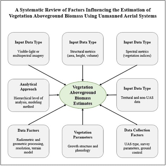
1. Introduction
The biomass of vegetation is the total mass of organic material representing the matter and energy assembled by photosynthesis of green plants [1,2]. Total biomass is often separated into belowground and aboveground biomass (AGB). Measurements of AGB are logistically easier to collect and are valuable in both agricultural [3,4,5] and non-agricultural settings [6,7,8,9].
In agricultural systems, AGB is a key agro-ecological indicator [4,10] that can be used to monitor crop growth, light use efficiency, carbon stock and physiological condition [3,5,6,11,12,13,14,15,16]; predict crop yield and ensure yield quality [2,3,5,12,13,14,17,18,19,20,21,22,23]; inform precision agriculture practices [3,15,21,22,23]; maximize efficiency of fertilization and watering [4,10,14,21]; detect growth differences among phenotypes or cultivars [10,23]; calculate nitrogen content and assess nutrient status of plants [24,25,26]; and optimize economic decision-making throughout the growing season [3,14,15,19,22,27].
In a non-agricultural context, estimation of AGB gives important insight into ecosystem structure and function. Forests, grasslands, wetlands, mangroves, dryland ecosystems and other vegetated areas provide important services for humans, such as carbon sequestration, oxygen production and biofuel, as well as habitat for plant and animal species [9,28,29,30]. Many ecosystems are also at increasing risk from climate change and land-use conversion and it is valuable to be able to quantify AGB at appropriate spatial and temporal scales and monitor it over time to assess the impacts of these changes on the global carbon cycle and to understand the resulting effects on ecosystem resilience and health [6,7,31,32]
AGB is most accurately measured by collecting and weighing samples of vegetation [3,19,33] but this method is time-consuming, labor-intensive and destructive [16,34,35]. Allometric equations that relate AGB to measurable biophysical parameters like diameter at breast height (DBH), plant height or canopy area provide a way to estimate AGB more efficiently but require genus- or species-specific equations that must be developed and calibrated with direct biomass information [36,37,38].
Remote sensing provides an alternative for estimating AGB at a variety of spatial scales [39,40,41,42]. Over the past decade, unmanned aerial aystems (UASs) have emerged as cost-effective remote-sensing tools for collecting very high-resolution data [18,25,43] with the potential to fill the gap between ground observations and traditional space- and manned-aircraft platforms [27,28,44]. A UAS consists of an aerial platform capable of autonomous or semi-autonomous flight, a sensor or sensors mounted on the platform that collects imagery at given intervals and a ground station from which flight parameters can be programmed and controlled [45]. UAS platforms can be programmed to accurately and precisely fly at given altitudes, speeds and directions with little to no input from a human operator during flight [46]. This makes UAS missions both reliable and repeatable, an advantage when there is a desire to survey the same area more than once [2,11,16,25]. UASs are also relatively inexpensive compared to other high-resolution remote sensing platforms [1,5,6,12,30,47,48,49,50], flexible in terms of operating conditions [5,22,43], compatible with a variety of sensors [1,5,6,15] and able to fly at low altitudes, thus reducing the impact of cloud contamination and atmospheric interference that often hinders satellite imagery [1,7,11,15,16,25]. These advantages have driven the rapid adoption of UASs as data collection tools in a variety of fields in recent years [45,51,52]. Although active sensors can be mounted on UASs for data collection, they are an evolving technology that is often still prohibitively expensive for many research applications and requires complex processing procedures to derive useful information from the data [8,48,53]. Passive sensor UAS imagery also has a higher point density than that from active sensors such as LiDAR [8,15], making it of greater utility to characterize small variations in plant structure. As a result, the applied-research domain on UAS-borne sensors is dominated by passive optical sensors that capture reflected electromagnetic energy in the optical wavelengths. These can be as simple as consumer-grade digital cameras or as complex as hyperspectral sensors that measure reflectance in hundreds of very narrow spectral wavelengths [54]. Such data provide information on the structure, texture and heterogeneity of vegetation canopies and are routinely processed into 3D point clouds using Structure from Motion (SfM) workflows [29,55,56]. This combination shows great promise for AGB estimation that is cost-effective, accurate and applicable to both agricultural and non-agricultural settings.
AGB estimation from UAS-derived optical data is still a fairly new area of research, although the number of publications on the topic is increasing rapidly. Despite increasing interest in AGB estimation from UAS data, this article represents the first systematic review on the topic. There is no standardized methodology for planning, collecting and analyzing these data to derive AGB information. Numerous factors related to data collection and analysis methods and the study species and area of interest have the potential to affect the accuracy and predictive capabilities of derived models [2,8,57,58]. Without careful consideration of these factors, AGB estimation may be biased or imprecise, resulting in decreased accuracy of AGB models with potentially negative consequences for inferences and management decisions made from this information. A comprehensive review of factors influencing AGB estimation accuracy is therefore valuable at this time to help researchers understand each stage of the process impacts results, so they can plan future data collection and analysis to produce the most accurate and robust models of vegetation biomass.
In this paper we summarize the peer-reviewed literature on using UAS-borne passive sensors for vegetation AGB estimation with the goal of increasing general understanding on how factors intrinsic to the study species and environment and data type, collection and analysis affect the accuracy of AGB modelling. Our goal was to synthesize key points from previous research to provide advice on optimizing each step of the procedure to produce the most accurate results and reveal areas where additional research is needed to answer questions that could not be resolved with this synthesis.
2. Methods
We performed a comprehensive literature search using Web of Science and Google Scholar databases to extract peer-reviewed studies related to estimation of vegetation biomass using UAS-borne passive sensors published before 28 August 2019. Keywords related to UASs (“unmanned”, “UAS”, “UAV”, “drone”, “unmanned aerial system”, “unmanned aerial vehicle”) and to aboveground vegetation biomass (“vegetation”, “biomass”, “plant”, “AGB”, “aboveground biomass”) were used in combination in the search until no additional studies were found.
To be included in the review, studies must have used (i) passive sensors borne on UASs to collect data and (ii) compared UAS-derived AGB estimates to a more direct method of AGB estimation—either allometric or directly-weighed measurements.
Since the goal of this review was to provide general advice to researchers looking to estimate AGB of whole plants in agricultural or non-agricultural environments, studies predicting parameters similar but not equivalent to biomass, such as volume, crop yield (if not the yield of the full plant) or forest growing stock, were not included in the review. However, there is a significant and growing body of literature looking at these parameters that may warrant a separate review, as they could be relevant to researchers interested in factors other than full-plant AGB.
Studies that estimated biomass from UAS data but did not report a coefficient of determination (R2) value for the accuracy of the relationship between UAS and direct biomass measurements were difficult to compare to the majority of studies, which reported R2 values and so were not included in the review. While the coefficient of determination can be biased by the presence of outliers or non-normality of the errors, it provides a valuable assessment of goodness of fit of a model’s ability to predict the response variable and is useful as a quantitative measure of the accuracy of predictive models of the relationship between remotely-sensed and ground-measured AGB [59]. We chose to only include papers reporting R2 values to allow some comparison among the accuracy of AGB estimation models.
While all of the papers selected for this review conducted model calibration (using all available data points to model the relationship between ground-measured and UAS-measured AGB), not all papers also conducted model validation, which we define as the application of the derived AGB estimation model to data not used to train the model. Model validation is useful for understanding how robust the model’s predictions are and is essential when there is an interest in applying models at different points in space or time. Since many of the vegetation AGB studies included in this review did not report on validation results, possibly due to their exploratory nature or to limited data available for validation, we report only R2 values from calibration models in our results. However, we urge researchers to conduct model validation when using UAS data to predict vegetation AGB as this will ensure the most robust, transferable results and hope that future studies include this important step in their workflow.
For each of the resulting studies that met our criteria, the following was assembled in tabular format (Appendix A)—study species and location, ground truth data type, UAS type, sensor type(s), flying height, photo overlap and sidelap, ground sample distance (GSD), whether analysis was done on an area-based plots or individual plants, spectral input data used, structural input data used, textural input data used, any other input data used, ground model source, model type(s) tested and best model(s) results. We will use the results of this synthesis to answer the following questions on how factors related to data collection, type, analysis and parameters of the study species and environment affect the ability to accurately estimate vegetation AGB:
- How well can structural data estimate vegetation AGB? Which structural metrics are best?
- How accurately can multispectral data predict vegetation AGB? Which multispectral indices perform the best?
- How well can RGB spectral data estimate vegetation AGB? Which RGB indices perform the best? How do RGB data compare to MS data? Is including RGB textural information useful?
- Does combining spectral and structural variables improve AGB estimation models beyond either data type alone?
- What other data combinations or types are useful?
- How do the study environment and data collection impact AGB estimation from UAS data?
- How do vegetation growth structure and phenology impact AGB estimation accuracy?
- How do data analysis methods impact AGB estimation accuracy?
We acknowledge that differences within the studies selected for our analysis could lead to challenges in comparing results directly. We guarded against this by not relying heavily on the quantitative results of any one paper. Instead, we sought to detect patterns emerging from groups of studies which we selected strategically from one question to the next. Cumulative bias arising from selective reporting or publication bias (only reporting positive results) could still be a factor.
3. Results and Discussion
We found 46 studies that fit the criteria of our review (Table A1). Geographic coverage of studies was widespread—two from Africa (Malawi), seven from North America (six from continental USA, one from Alaska), one each from Central and South America (Costa Rica and Brazil), 16 from Europe (Germany—8, Belgium—2, Spain—2 and one each from Finland, Norway, Portugal and Switzerland) and 19 from Asia (China—15, Japan—2, India—1, Myanmar—1).
The earliest published recognition of the utility of UASs for biomass estimation was 2005 [60], followed by no further publications until 2013. Since then the number of peer-reviewed studies on UAS-based vegetation biomass estimation fitting the criteria of this paper has grown steadily, with 19 published in 2019 before the end of August alone (Figure 1).
In general, studies followed a similar workflow to derive estimates of vegetation AGB from UAS data, summarized in Figure 2. While not every study utilized every step, the overall process was common to many of the vegetation AGB research projects included in this review. The workflows usually involved the following steps—(1) collection of UAS imagery concurrent with ground-based AGB data collection, either using allometric or direct (destructive) sampling; (2) data processing, including pre-processing, creation of photogrammetric 3D point clouds and/or orthomosaics, georeferencing of point clouds and orthomosaics, creation of canopy height models using digital terrain and digital surface models, delineation of individual areas or plants of interest in models and derivation of structural, textural, and/or MS, HS or RGB spectral variables; (3) creation of predictive AGB models using UAS-derived variables as predictors and ground-based AGB as the response variable, followed by variable selection, assessment of accuracy of the top model and in some studies, validation of the top model; and (4) in some studies, an application of the top model to estimate site-wide biomass.
3.1. Input Data
The choice of parameter(s) derived from UAS imagery is likely the most important factor influencing the accuracy and predictive ability of AGB estimation. Some studies used spectral information [2,11,18,24,26,43,58,60,61,62] and some structural information [1,8,22,23,28,34,48,50,55,63,64,65]. Others used both [3,4,5,6,9,12,16,20,21,25,30,33,49,57,66,67,68], while a few studies used spectral and structural metrics plus another data type [13,27,69] (Table A1). Within these categories, a wide range of species, study areas and methods are examined, demonstrating the applicability of UAS data to AGB estimation in agricultural and non-agricultural environments.
The very high spatial resolution of UAS-derived imagery, often producing centimeter to sub-centimeter pixel sizes, means that it is possible to derive measurements of vegetation structure at much finer scales than with conventional remotely-sensed data. Normally, individual plants and even plant parts can be detected in UAS images. This provides a way to measure physical parameters of vegetation such as height, area and volume which can be related to vegetation AGB. While a small number of studies use structural metrics calculated directly from 3D photogrammetric point clouds, a more typical workflow for deriving structural data from UAS imagery involves creating a Digital Surface Model (DSM), representing the surface of the vegetation canopy and a Digital Terrain Model (DTM) representing the location of the ground in the image, including beneath the vegetation canopy. By subtracting the values of the DTM from the DSM, a Canopy Height Model (CHM) representing the difference in height between the canopy of the vegetation and the ground can be created and metrics of vegetation structure can be extracted from the CHM at the plot or individual plant level and related to ground-based AGB measurements.
It has long been recognized that vegetation shows characteristic patterns of absorbance or reflectance of light in certain wavelengths and that these patterns can be exploited to measure biophysical parameters of plants [70,71]. Satellite remote sensing of AGB usually uses multispectral (MS) information to derive AGB estimates and some UAS studies have done the same. Additionally, the recent increase in the use of visible-light sensors such as consumer digital cameras borne on UASs means there has been a concurrent increase in the development and application of vegetation indices (VIs) using only the visible (RGB) wavelengths imaged by these sensors [72].
In addition to spectral vegetation indices, information in the texture of image features can also be derived from RGB or MS data. Texture contains important spatial information regarding the structural arrangement of vegetated and non-vegetated surfaces in the image and their relationship to the surrounding environment [73].
The following sections of this review will compare and discuss the influence of UAS-derived input data type(s) on AGB model accuracy, using the coefficient of determination statistic (R2) as the main indicator of model performance. For the purposes of this study, we consider R2 values between 0 and 0.25 to indicate a poor relationship; values from 0.25 to 0.5 to indicate a moderate relationship; values from 0.5 to 0.75 to indicate a good relationship; and values greater than 0.75 to indicate an excellent relationship. Our goal was to answer key questions with regards to the performance, accuracy and reliability of each data type in the context of AGB estimation.
3.1.1. How Well Can Structural Data Estimate Vegetation AGB? Which Structural Metrics Are Best?
We found 15 research papers [1,8,19,22,23,28,34,48,50,55,62,63,64,74,75] that used structural measurements alone and 12 papers [4,5,9,12,15,16,20,21,25,30,49,57] that used structural metrics along with spectral data to estimate biomass of vegetation (Table A1). All structural variables used by studies in this review are listed in Table 1. Reported coefficients of determination ranged from 0.54 from a study estimating rye and timothy grass pasture AGB using mean plot volume [64] to >0.98 from a study estimating coniferous tree AGB from tree height metrics [1], indicating that structural metrics alone derived from UAS imagery can be used to estimate vegetation AGB with moderate to excellent accuracy depending on study species and methodology. All studies using structural metrics alone used RGB imagery to derive metrics representing on vegetation structure.
Mean, median and maximum height metrics provide information on the vertical distribution of the vegetation canopy [3,69]. Maximum or median height appear to be particularly useful for trees. Lin et al. [1] found a very strong relationship between maximum coniferous tree height derived from a CHM and allometric measurements of tree biomass (R2 = 0.99) and Guerra-Hernandez et al. [50] found that maximum tree height and crown area estimated from a CHM had a very strong relationship with pine tree AGB (R2 > 0.84). Zahawi et al. [48] found that median height in a linear model strongly predicted tropical tree AGB (R2 > 0.81), better than other height metrics or measures of canopy proportion, roughness and openness. While Dandois et al. [55] reported a very good relationship between mean canopy height and allometric AGB of deciduous trees (R2 = 0.80), they noted error in AGB representing over 30% of total site biomass, so these estimates were not highly precise.
For non-woody plants, mean height appears to be useful. Bendig et al. [23] found similar accuracies for fresh (R2 = 0.81) and dry (R2 = 0.82) biomass of barley crop plots using mean canopy height in an exponential model, while Willkomm et al. [74] found that fresh rice AGB could be estimated with higher accuracy (R2 = 0.84) than dry biomass (R2 = 0.68) using mean height in a linear model. Grüner et al. [19] found that, when grouped, grass species showed a good relationship between mean canopy height and ground-level AGB measurements (R2 = 0.73) but that individual species models had variable accuracy (R2 = 0.62–0.81). Zhang et al. [65] found that a logarithmic regression using mean height had an excellent relationship with grasslands biomass (R2 = 0.80).
Combining mean or maximum height variables with other spectral and/or structural metrics was found to be useful by some researchers. Ota et al. [49] reported that mean height, along with 60th percentile of height, was retained in their top model for tropical tree AGB estimation (R2 = 0.77), while Kachamba et al. [30] found that maximum height was the most frequently selected variable in their candidate set of models for tropical tree AGB and was retained in the best model (R2 = 0.67), along with one spectral and one other structural variable. Mean height was retained in the top model for aquatic plant biomass estimation [9], along with three spectral and two other structural metrics, with very good model performance (R2 = 0.84). Cen et al. [5] found that mean height was the second-most important variable in their highly-accurate random forest model (R2 = 0.90) for estimating maize biomass, while Li et al. [15], also looking at maize biomass, found that mean height was retained with two other structural and two spectral variables in their top model with good accuracy (R2 = 0.78).
However, in some situations mean, maximum and median height metrics may lead to underestimation of canopy height as it is difficult to capture the very top of vegetation in point clouds [19,23] and soil visible through the canopy can reduce mean height measurements [16]. Height variables other than mean or maximum may better capture the variation of canopy height within a plot. Rather than mean canopy height, Acorsi et al. [75] calculated the average maximum height at the plot level in an attempt to accurately capture plot-level variations in height during the lodging stage of oats, when plants start to bend over due to biomass accumulation in top-heavy reproductive organs. This study found that good to excellent accuracy was achieved when estimating fresh and dry oat biomass, although coefficients of determination varied across the growing season (R2 = 0.69–0.94) [75].
Two studies found that combining multiple height metrics was the best approach to AGB estimation. Jayathunga et al. [28] reported that a random forest model combining five height metrics had better performance (R2 > 0.87) than linear regression models with one to three height metrics (maximum R2 = 0.78) for estimating temperate tree AGB. Similarly, Moeckel et al. [34] used a random forest model encompassing 14 canopy height metrics to estimate the biomass of eggplant, tomato and cabbage crops, finding very high accuracies for all three crop types (R2 = 0.88–0.95).
Percentiles of height and metrics such as the coefficient of variation (CV) or standard deviation (SD) of mean height can also be useful because they shed light on the horizontal and vertical complexity and heterogeneity of the canopy [13,15]. Wijensingha et al. [63] found 75th percentile of height was the best among the ten height variables compared, producing moderate accuracy in grassland AGB estimation from linear regression models (R2 = 0.58–0.62). Ota et al. [49] found that the combination of mean height and 60th percentile of height produced the most accurate model (R2 = 0.77) for tropical tree biomass estimation among the 14 structural and 4 spectral metrics tested, while Roth and Streit [21] found the 90th percentile of height could predict cover crop AGB with good accuracy (R2 = 0.74), outperforming spectral and canopy cover metrics. The best model found by Domingo et al. [57] for tropical tree AGB estimation contained the variables 80th percentile of height, 20th percentile of canopy density and skewness of height, outperforming 105 spectral and 83 structural variables (R2 = 0.76).
Several studies using both spectral and structural data also had height CV, SD or percentiles frequently retained in top models. In one study the 90th percentile of height was retained along with maximum height and a spectral metric in tropical tree AGB biomass models with good accuracy (R2 = 0.67) [30]. The SD and CV of height were retained in the best model for aquatic plant biomass estimation along with mean height and two spectral variables, achieving very good model accuracy (R2 = 0.84) [9]. Jiang et al. [13] found that the CV of height outperformed all other height and spectral metrics tested in single variables models for rice biomass estimation (R2 = 0.77) and CV of height was retained in the top multivariate model as well (R2 = 0.86). The 50th percentile and CV of height were retained in the top multiple linear regression model (R2 = 0.81), along with spectral and meteorological data, for ryegrass AGB estimation [69], outperforming mean and maximum height metrics. Variables representing the complexity and heterogeneity of vegetation canopies along vertical and horizontal axes appear to be especially useful when combined with other structural and/or spectral data in multivariate models for AGB estimation.
Metrics representing canopy volume capture variation in vegetation height and density simultaneously [22]. Rueda-Ayala et al. [32] used mean plot volume to estimate AGB of rye and timothy pastures in a linear regression model but found relatively low accuracy (R2 = 0.54) compared to the rest of the papers in this section, although this study did not use a terrain model and estimated heights from a canopy surface model alone which may have decreased model performance. Other studies reported better results using volume: Ballesteros et al. [22] compared canopy volume, height and cover metrics for measuring onion crop AGB as well as bulb biomass using exponential regression models, finding that volume performed better to predict leaf biomass (R2 = 0.76) than canopy height or area. Canopy volume was found to be the most important predictor among 11 spectral and 3 structural metrics tested for estimation of maize crop AGB, resulting in a very accurate model (R2 = 0.94) [16]. Volume estimates can be useful for woody vegetation as well: Alonzo et al. [8] used the 75th percentile of tree height and crown width at median tree height to calculate tree crown volume and found an excellent relationship with tree AGB (R2 = 0.92) at the individual tree level. Finally, combining volume with spectral data showed promise in one study for very accurate AGB estimation from a single variable. Maimaitijiang et al. [3] found that a regression model containing only a metric representing canopy volume weighted by an RGB VI had nearly as good a model performance (R2 = 0.89) as a regression model containing all tested spectral and structural variables (R2 = 0.91) for soybean AGB estimation, representing an intriguing development that warrants further study.
3.1.2. How Accurately Can Multispectral Data Predict Vegetation AGB? Which Multispectral Indices Perform the Best?
We found seven studies [11,18,24,43,58,61,62] that used MS or hyperspectral (HS) data alone and seven studies that combined MS or HS data with structural data [5,6,16,20,21,57,67] to measure AGB (Table A1). All MS or HS data and their calculation formulas used by studies considered in this review are shown in Table 2. The lowest reported coefficient of determination among the studies using MS and HS to estimate AGB was 0.36 for wetland vegetation biomass calculated across all seasons, although this study found higher accuracy when data were not pooled seasonally. The highest R2 value was 0.94 reported by two studies, one estimating tallgrass prairie biomass [77] and one looking at maize crop biomass with MS and RGB spectral and structural data [16].
Indices that incorporate the near infrared (NIR) region of the electromagnetic spectrum were commonly used for vegetation biophysical parameter estimation. Fan et al. [18] took a simple approach to ryegrass AGB estimation by simply adding the digital numbers (DNs) from each of the red, green and NIR wavelengths imaged within each study plot and found an excellent relationship with biomass (R2 = 0.84), with the NIR band having the highest correlation with biomass. This result shows that a straightforward AGB modelling approach using high-resolution (2 cm pixels) MS data can produce accurate biomass estimation models. Rather than using the DNs from single MS bands, though, most of the research papers used NIR data in vegetation indices combining two or more wavelengths of light. Yuan et al. [11] tested four NIR-based VIs for their ability to estimate cover crop biomass and found that good to excellent model accuracy could be achieved with all four VIs, although R2 values and which VI was most important varied among the four fields studied (R2 = 0.60–0.92). Zheng et al. [26] used RGB, red edge and NIR indices along with textural data to estimate AGB and found that the NIR data outperformed the other two VI types at all growth stages of rice (max R2 = 0.86).
NDVI, a VI that contrasts the reflectance of red and NIR wavelengths of light to reveal the volume of chlorophyll pigments [79], is frequently used for assessment of vegetation biophysical parameters. Ni et al. [76] compared UAS-based NDVI to NDVI measured with a ground sensor and found an excellent relationship between the two parameters (R2 = 0.77), demonstrating that aerial estimates of NDVI are similar to what can be measured on the ground with the advantage of collecting data over a much broader area. Wang et al. [62] used NDVI from a three-band MS sensor collected at three different flying heights to estimate AGB in a tallgrass prairie, finding excellent relationships with biomass at three different flying heights (R2 = 0.86–0.94) with the strongest relationship at the lowest flying height.
Some researchers found that NDVI could outperform other MS indices. Geipel et al. [24] compared NDVI to REIP for estimation of winter wheat AGB and found that among the four fields studied, NDVI best predicted biomass in three fields (R2 = 0.72–0.85), while Yuan et al. [11] found that NDVI best predicted cover crop biomass in two out of four fields studied compared to three other NIR-based indices. Doughty & Cavanaugh [43] found that NDVI was the best VI for coastal wetland vegetation AGB measurement, although model performance varied widely among seasons with the best performance during the spring (R2 = 0.36–0.71). NDVI was one of three spectral indices retained, along with three structural metrics, in the best model for maize biomass estimation, resulting in a very strong relationship with maize AGB (R2 = 0.94) [16].
Conversely, Honkavaara et al. [61] found that hyperspectral data from 42 narrow bands predicted wheat AGB better (R2 = 0.80) than NDVI alone (R2 = 0.57–0.58), although the data used in this study had a lower spatial resolution (20 cm) than other MS studies and was the only research to calculate NDVI from narrow-band hyperspectral data. Peña et al. [67] found that an index created by multiplying tree height by NDVI had only a moderate relationship with tree AGB (R2 = 0.54) but this study calculated tree height from a DSM without any terrain data, which likely lowered model performance. Yue et al. [6] obtained better results multiplying hyperspectral bands and indices by plant height, calculated using a CHM, for estimating wheat AGB (R2 = 0.78), with their top model including NDVI along with seven other indices multiplied by height. While the performance of NDVI and other NIR-based indices depends to some degree on factors external to the data themselves, such as vegetation species and phenology or survey flying height, UAS-derived NIR indices can produce accurate models of vegetation AGB either alone or combined with other data.
The red-edge wavelength, a narrow region of the spectrum between red and NIR wavelengths [71], is available on many MS sensors designed for UASs. Red-edge VIs have a strong relationship with leaf biomass and weaker relationship with stem biomass [13,26] and are sensitive to canopy structure [62], making them useful for AGB estimation for vegetation species with large leaves or for growth stages of plants when the canopy is dominated by leaves. Red-edge indices may also be slightly less prone to saturating in dense vegetation than those using the NIR band [21] and several studies found that red-edge indices could predict vegetation AGB with similar or higher accuracy than NIR indices. The red-edge VI REIP outperformed NDVI for one of the four wheat fields studied by Geipel et al. [24] and had good performance at the other three fields (R2 = 0.70–0.81), while Ni et al. [58] found a slightly higher linear relationship between wheat AGB and the Ratio Vegetation Index (RVI) using bands at 720 (red edge) and 810 (NIR) nm (R2 = 0.66), compared to NDVI (R2 = 0.62). Wang et al. [62] found that VIs using red-edge bands were more important than other indices, including NDVI, for rice AGB estimation during whole season (R2 = 0.72–0.74) and pre-heading (R2 = 0.74) growth stages in linear mixed effects models, similar to Zheng et al. [26] who reported red-edge indices yielded the best performance out of all MS indices tested for rice estimation during pre-heading stages (R2 > 0.70). Jiang et al. [13] found that red-edge based indices were the top three indices in single-variable models and that the normalized difference red edge (NDRE) index was in the top multivariate model for whole season rice AGB estimation (R2 = 0.86), achieving accuracy almost as good as a random forest model containing all variables (R2 = 0.92). Data in the red-edge wavelength appears to have equivalent utility to the NIR for vegetation biomass estimation from UAS imagery and is possibly more useful for vegetation types with dense canopies where NIR would saturate and for earlier stages in the growing season of non-woody vegetation.
3.1.3. How Well Can RGB Spectral Data Estimate Vegetation AGB? Which RGB Indices Perform the Best? How do RGB Data Compare to MS Data? Is RGB Textural Information Useful?
We found two studies [2,60] that used RGB spectral data to predict AGB and 14 studies [3,4,5,9,12,15,16,20,25,30,49,57,66,68] that combined RGB spectral and structural data for biomass estimation (Table A1). All RGB metrics and their calculation formulas used by studies considered in this review are shown in Table 3. With the reported coefficients of determination ranging from 0.39 to >0.90, information from RGB sensors shows promise for estimation of vegetation AGB.
When comparing three crop types, Hunt et al. [60] found that the Normalized Green-Red Difference Index (NGRDI) could predict corn AGB most accurately (R2 = 0.88), followed by alfalfa (R2 = 0.47) and soybean (R2 = 039). This study was the earliest publication on AGB estimation from UAS-derived imagery (2005) and it is likely that improved model performance could be achieved using today’s more advanced UASs and sensors with a higher spatial resolution than were available when the study was published. In addition to RGB spectral data. Yue et al. [2] included textural information derived from RGB imagery in their models, finding very good model performance for predicting winter wheat AGB (R2 = 0.82–0.84) using two RGB VIs, VARI and red ratio and one texture metric.
Many researchers found that combining RGB VIs with structural data also derived from RGB imagery produced models with good accuracy. Kachamba et al. [30] found that the SD of the RGB blue band was retained along with two structural metrics in their top model for tropical tree biomass estimation with good accuracy (R2 = 0.67). For aquatic plant AGB estimation, the RGB VIs NGRDI and Excess Green Index produced very high model accuracy (R2 = 0.84) along with three height metrics. Cen et al. [5] found that seven of the eight top variables in their rice biomass prediction model were RGB VIs in a highly-accurate model (R2 = 0.90). Yue et al. [20] reported than a random forest model combining three RGB bands, nine RGB indices and plant height could predict wheat AGB with very high accuracy (R2 = 0.96) and that a simple regression including only plant height and red ratio could also achieve very good model accuracy (R2 = 0.77). Also for wheat, Schirrman et al. [25] found that combining four RGB VIs with plant height and crop area could predict fresh and dry biomass with good to very good accuracy (R2 = 0.70–0.94), with model performance depending on the timing of data acquisition. Niu et al. [4] reported that three RGB VIs and plant height were retained in the top multiple linear regression model for maize biomass estimation, resulting in high accuracy for both fresh and dry AGB (R2 = 0.85 for both). Han et al. [16] found excellent model performance (R2 = 0.94) combining two RGB VIs with three RGB structural metrics and NDVI in a random forest model for estimating biomass of maize, while Lu et al. [12] reported slightly lower, although still good (R2 = 0.76), random forest regression model performance when combining 10 RGB spectral indices and eight height metrics for wheat AGB estimation.
Several studies found that when compared, RGB VIs could outperform MS or HS information in AGB models. Roth and Streit [21] reported that, for the cover crop species studied, the RGB-based Green Red Vegetation Index (GRVI) had higher correlations to dry biomass and was more important in linear mixed effects models than NIR or red-edge-based VIs. Han et al. [16] found that RGB VIs NGRDI and VARI were retained with higher importance than NDVI in a random forest regression-based maize estimation model. Similarly, Cen et al. [5] found that seven RGB VIs, along with plant height, were more important predictors for rice AGB estimation in a random forest regression model than three ratio-based MS VIs. For winter wheat AGB estimation, RGB data performed slightly better than hyperspectral information in both linear (RGB R2 = 0.77; HS R2 = 0.74) and random forest (RGB R2 = 0.96; HS R2 = 0.94) regression models [20]. In general, RGB imagery collected had a higher spatial resolution than MS or HS imagery, which may have influenced its ability to more accurately predict vegetation biomass.
Among all the studies that used RGB data to estimate vegetation AGB, a total of 32 different RGB VIs were tested (Table 3). Various RGB VIs were retained in top models in different studies depending on study species, analysis methodology and which VIs and other data were tested, making it difficult to determine which RGB VIs are most important for general biomass modelling. However, some patterns on which VIs could best predict AGB did emerge and it appears all three RGB bands can be useful for biomass modelling. The Normalized Green-Red Index (NGRDI) was the most frequently retained in top models among all the RGB VIs tested, found in nine best models after variable selection [3,4,5,9,12,15,16,27,60] and two ensemble random forest models [3,27]. The NGRDI may be particularly sensitive to biomass estimation in non-woody vegetation before canopy closure [60], making it useful for modelling of herbaceous vegetation in earlier parts of the growing season. Simple ratio-based indices using a combination of two RGB bands in the formula band 1/band 2, especially those using the red and green bands, were found to be important in top models from multiple studies [3,5,20,25], potentially because ratio-based VIs may be less sensitive than other VIs to changes in illumination and atmospheric conditions over time [3]. The modified red-green ratio index (MGRVI) was important in both studies in which it was included [5,25], while Kawashima’s Index (IKAW), a normalized index using red and blue bands, was also important in the two studies in which it was tested [3,12]. Several indices using all three RGB bands were found in top multivariate or ensemble models in more than one study, including VARI [3,5,12,16,20,27], Excess Green-Red Index [3,4,9,12], Excess Green Index [3,12,15], Excess Red Index [3,12,20], VEG [3,4,5], VDVI/GLI [3,5,12], RGBVI [12,66], Excess Blue Index [3,12] and red, green and blue ratio indices [3,20]. Finally, two studies found that using the SD of single-band or VI values within a unit area were the most important spectral variables in AGB estimation models [30,69], indicating that a measure of spectral variability may also be valuable for biomass modelling.
Two studies (Table A1) incorporated textural analysis derived from RGB data along with spectral indices to estimate herbaceous crop AGB from UAS imagery. Both reported improved performance, despite finding that different texture measurements were most important to their AGB models. Both papers compared the performance of eight common texture metrics derived from a grey-level co-occurrence matrix (GLCM)—mean, contrast, homogeneity, variance, dissimilarity, entropy, second moment and correlation [2,26]. Yue et al. [2] used RGB VIs plus metrics of image texture at multiple spatial resolutions to estimate the AGB of winter wheat and found that including image texture variables along with VIs led to an increase in R2 values (0.84) compared to VIs (max R2 = 0.76) alone. The strength of the relationship between texture variables and AGB depended on the both the growth stage of the plant and on the spatial resolution of the texture measurements, with 1-cm and 30-cm resolution textures having the strongest relationships with AGB [2].
Zheng et al. [26] utilized measurements of texture plus the Normalized Difference Texture Index (NDTI) and found that integrating NDTIs with VIs in a stepwise multiple linear regression improved model performance (R2 = 0.78) compared to either metric alone (VI max R2 = 0.63; texture max R2 = 0.56), both for whole-season and individual growth stage models. This study also reported better performance using NDTIs compared to single-band texture measurements [26], which is important for researchers interested in incorporating texture measurements in vegetation AGB models, especially for species such as rice that has a less homogeneous canopy than wheat. Including texture may help to overcome the problem of underestimation of AGB at high biomass values can occur when measuring AGB using VIs alone [2].
3.1.4. Does Combining Spectral and Structural Variables Improve AGB Estimation Models Beyond Either Data Type Alone?
One of the main advantages of UASs for data collection is their ability to collect imagery with a single survey from which both spectral and structural parameters can be derived. Combining multiple UAS-derived data types has the potential to improve the estimation of vegetation AGB because they capture variability in the spectral and structural attributes of the vegetation canopy since they measure both biochemical and biophysical properties of plants [10,12,40]. We found 17 studies [3,4,5,6,9,12,15,16,20,21,25,30,49,57,66,67,68] that combined spectral and structural information to estimate vegetation AGB from UAS imagery (Table A1) with coefficients of determination ranging from 0.54 to >0.95.
In some cases, metrics of vegetation structure outperformed spectral indices for AGB estimation. Two studies found that for tree biomass estimation, only structural metrics were necessary to produce models with good accuracy. Ota et al. [49] used a change-based approach for tropical tree AGB estimates and found the most accurate model was created using RGB-imagery-derived mean height and 60th percentile of height of each measured plot, with none of the four RGB VIs tested included in the best model (R2 = 0.77). Domingo et al. [57] compared structural and spectral data derived from MS and RGB imagery for estimating tree biomass in a tropical forest, finding that height metrics from the RGB camera produced models with higher accuracy (R2 = 0.76) than RGB or MS spectral data (max R2 = 0.66). In one study on mixed-species fields of cover crops, structural data also outperformed spectral information. Roth & Streit [21] found only 90th percentile of height was needed to predict the biomass of mixed-species cover crops with good accuracy (R2 = 0.74), although the strong relationship between plant height and biomass only applied to some of the species studied.
However, most studies using spectral and structural information to estimate AGB reported that both types of data were retained in the best models, indicating the two data types can complement each other in biomass estimation models. Combining structural data, such as height metrics with vegetation indices in the same model, can help avoid or overcome issues of spectral saturation [13,22]. For example, Jiang et al. [13] found that the performance of NDVI was lower (R2 = 0.41) than NDRE (R2 = 0.64) when each was included in single-variable linear models but that the difference in estimation accuracy between the two was reduced when combined with a height metric (NDVI R2 = 0.79; NDRE R2 = 0.83), indicating that combining NIR VIs with structural information may relieve the saturation of NDVI after canopy closure. Han et al. [16] found excellent accuracy in maize biomass estimation (R2 = 0.94) from a random forest model containing two structural and four spectral variables. Li et al. [15] also used a random forest model to estimate maize AGB with a combination of spectral and structural variables with good accuracy (R2 = 0.78). Kachamba et al. [30] created 13 models for tropical tree AGB estimation, finding that all models (R2 = 0.67–0.85) contained at least one structural and one spectral variable. Schirrmann et al. [25] found that both spectral and structural variables were important in the principal components used to estimate fresh and dry biomass of winter wheat high accuracy (R2 = 0.70–0.97) in a multiple linear regression, with plant height and ratios, including the blue band, being the most important.
When compared directly, several studies found that the including both data types at least slightly improved model performance over models with either data type alone. Niu et al. [4] found that a model combining plant height and RGB VI metrics had a higher R2 (0.85) than models using only plant height (R2 = 0.77) or VIs (R2 = 0.82). Similarly, Jing et al. [9] found that aquatic plant AGB could be estimated with higher accuracy using a combination of spectral and structural data (R2 = 0.84) compared to either height metrics (R2 = 0.73) or VIs (R2 = 0.79) alone, while Lu et al. [12] reported slightly improved model accuracy (R2 = 0.76) when estimating wheat AGB using a random forest model combining all spectral and canopy height metrics derived from RGB imagery versus VIs (R2 = 0.70) or height metrics (R2 = 0.73) alone. Cen et al. [5] found that combining all RGB and MS indices with mean height into a random forest model increased the accuracy of rice AGB estimation (R2 = 0.90) compared to single variable models using plant height, RGB or MS VIs (R2 ≤ 0.53). Yue et al. [20] estimated the AGB of winter wheat and found that a random forest model with all RGB VIs and crop height was the most accurate approach for modelling AGB (R2 = 0.96), outperforming single-variable models using VIs (R2 = 0.57–0.74) and height (R2 = 0.03–0.73). In general, it appears that including both spectral and structural data in vegetation biomass estimation models can overcome the limitations of each data type and usually improves model performance to a degree dependent on factors such as study species, phenology and analytical method.
3.1.5. What Other Data Combinations or Types Are Useful?
Five studies [3,6,66,67,68] examined whether combining spectral and structural UAS information into a single metric could improve AGB estimation accuracy. One study found that this approach did not result in better AGB models. Possoch et al. [68] compared the Grassland Index (GrassI), calculated as mean height plus the RGBVI*0.25, to height and RGBVI alone for estimating grassland biomass, and found lower accuracy for the GrassI model (R2 = 0.48) versus the mean plot height model (R2 = 0.64), although GrassI did significantly outperform RGBVI alone (R2 = 0.0012). However, this study used a sensor with a fisheye lens, which the authors note may have affected the accuracy of their results and only examined one VI; combining canopy height with a different VI or using a sensor with less lens distortion, may have produced more accurate models.
The other four studies applying this method found that it improved AGB estimation models. Peña et al. [27] reported that a linear regression including NDVI multiplied by mean height had higher accuracy for estimating poplar tree AGB (R2 = 0.54) than height (R2 = 0.44), tree volume (R2 = 0.34) or NDVI (R2 = 0.24) alone. Bendig et al. [66] found that for barley AGB, adding RGBVI multiplied by plant height into quadratic regression models improved accuracy (R2 = 0.84) compared to VIs (max R2 = 0.74) or plant height (R2 = 0.80) alone. Yue et al. [6] estimated winter wheat crop biomass and found that accuracy of models including both spectral and structural information in one measurement was higher (R2 = 0.78) than models with single measurements of height (R2 = 0.50) or spectral metrics (max R2 = 0.59). Maimaitijiang et al. [3] compared canopy volume weighted by various RGB vegetation indices to spectral or structural data alone for determining soybean AGB and found that a linear regression model using only volume weighted by the GRRI had nearly as high accuracy (R2 = 0.89) for estimating AGB for all combined measurement dates as a stepwise multilinear regression using all 20 RGB spectral parameters and 6 canopy height metrics (R2 = 0.91). The finding that canopy volume weighted by a VI outperformed VIs or canopy volume alone led the researchers to conclude that while canopy volume, which represents both vertical and horizontal properties of vegetation canopy, has a good relationship with AGB, multiplying it by a VI can improve the accuracy of AGB estimation as spectral information can capture differences in crop physiology, species and genotypes to provide supplementary information for measuring AGB beyond volume alone [6]. The good results found by most studies in this section indicate that when both spectral and structural information are available, it is worth testing a metric combining the two in AGB models to see if accuracy can be increased compared to either alone.
We also found three studies [13,27,69] that utilized UAS-derived spectral and structural information along with another measurement (Table A1), with all three reporting that biomass estimation accuracy was improved with the inclusion of these data. While collecting extra non-UAS ancillary data increases the amount of effort involved in AGB estimation, if it has the potential to improve model accuracy it may be worth the additional work.
Two of these studies added meteorological information to spectral and structural metrics. Jiang et al. [13] used spectral, canopy height and growing degree day (GDD) data to estimate the AGB of rice crops, finding that the best linear regression model (R2 = 0.83), combining height and a red-edge VI, could be improved slightly with the addition of meteorological information in the form of GDD (R2 = 0.86) and the highest R2 was achieved when all three data types were combined in a random forest model (R2 = 0.92). The authors concluded that combining red-edge VIs, which have been shown to have a strong relationship to biomass while being less prone to saturation at high biomass than NDVI, with a measure of canopy roughness and GDD could produce highly accurate estimates of rice biomass, although they emphasize the influence of plant growth stage and choice of model type on the results [13]. Borra-Serrano et al. [69] also included GDD, as well as change in GDD since the previous measurement, in ryegrass AGB estimation models along with 10 spectral indices and seven canopy height metrics. They found that a multiple linear regression including spectral + structural + GDD + ΔGDD (R2 = 0.81) outperformed all other models (max R2 = 0.71) [69]. Given the strong influence of temperature and climate on plant biophysical parameters and the possibility of changes in plant productivity related to these factors over short periods of time [33], if meteorological information is available for the study area of interest, it can be valuable to include in AGB estimation models.
Adding ground-based biomass measurements to UAS-derived data has also been tested by two studies. While Borra-Serrano et al. [69] found decreased model accuracy after adding a ground-based biomass measurement collected from a rising plate meter to their best model, Michez et al. [24] found that including interpolated maize AGB estimates based on ground-measured data improved model performance (R2 = 0.80) compared to estimates with no ground-based data (R2 = 0.55), especially later in the growing season. Since different crop types were examined and different modelling methods were used between the two studies, it is difficult to determine why these differences were found but the differences in ground AGB estimation method between the two studies—rising plate meter in Reference [69] versus direct measurements followed by interpolation to plot level in Reference [27]—may help explain this result. For study species and areas where ground-based AGB data is available, it can improve biomass estimation model accuracy, although the utility of including ground-based AGB data varies throughout the growing season, with the greatest improvement in model accuracy using late-growing-season ground data [27].
3.2. Other Factors Influencing AGB Estimation
In the remainder of this review we will focus on evaluating additional factors that influence the accuracy and predictive ability of models that estimate vegetation AGB from UAS-borne passive sensor imagery. These are organized into three main categories: characteristics of the study site and data collection methods, characteristics of the vegetation being studied and factors related to data analysis. When relevant, we will compare the effects of each parameter on spectral and structural data; otherwise we will consider both data types together. While it is difficult to compare absolute values of coefficients of determination and therefore the accuracy of AGB estimations from different studies since differences in the vegetation being studied and methods of collecting and analyzing data preclude direct comparison, relative comparisons will be made among studies to find general patterns in which factors are most influential to AGB measurement. In cases where researchers do examine within the same study how differences in any of these factors affect AGB estimation accuracy, we will report on results and discuss how these differences influence biomass measurement and prediction.
3.2.1. How do the Study Environment and Data Collection Impact AGB Estimation from UAS Data?
Parameters related to data collection and the environment being studied have the potential to impact model results, no matter the type of data included in AGB estimation. Researchers must consider how the UAS platform and sensor being used as well as the study site and environmental conditions could impact the imagery collected, data derived and results and inferences made related to biomass measurements.
Data Collection
With an increasing number and variety of platforms available on the market, ranging from small and inexpensive consumer-grade drones to highly-specialized aerial vehicles designed explicitly for research, choosing a UAS platform depends on budget, which sensor(s) will be carried and where the research is being conducted. Many UAS studies use multirotor platforms due to their high stability, superior image quality and good control [78]. However, multirotor platforms tend to require more energy to fly due to their vertical takeoff and landing and ability to hover, leading to lower endurance and shorter flight times [78] and if survey height is low, backwash from the rotors may impact the vegetation being studied by causing movement of plants [74]. In contrast, fixed-wing platforms can fly at higher speeds and for longer times, allowing them to cover larger areas more efficiently but have lower stability, which can impact image quality. Fixed-wings also have more complex operation, such as needing a runway or similar area to take off and land [78]. Overall, we found no discernible pattern in AGB estimation model accuracy between studies that used fixed-wing and multirotor platforms and suggest that the choice of UAS platform depends on the research needs. If the area to be studied is large and stability less of a concern, a fixed-wing will be more efficient. For smaller, complex areas where vertical takeoff and landing is necessary or if there is a need for detailed vegetation imaging from a highly-stable platform, a multirotor would be a better choice.
Like the choice of UAS platforms, selecting a sensor or sensors to be used depends on budget and desired applications, with each type having innate advantages and drawbacks. When comparing different sensor types for measuring biophysical parameters of vegetation, several researchers found that RGB data from inexpensive digital cameras resulted in AGB estimates with similar or higher accuracy than data derived from more expensive MS or hyperspectral sensors [5,20,57]. However, consumer-grade RGB digital cameras are subject to spectral, geometric and radiometric limitations such as distortions and “hot spots” in images caused by light on reflective surfaces, which require correction [80,81,82]. The construction quality of consumer-grade digital cameras can lead to vignetting caused by increased light obstruction and differences in light paths between the center and edges of the lens, resulting in a radial shadowing effect at the image periphery which should be corrected in order to preserve spectral and structural attributes of data near the edges of the imagery [24,25,80]. While the spatial resolution of digital cameras is much higher than most satellite-borne sensors, they lack the spectral resolution of multi- or hyperspectral sensors and digital cameras have a high degree of overlap between bands in the visible portion of the spectrum, meaning data is of limited use for quantitative vegetation analyses designed for MS data that require specific bands for calculating indices [83]. When specific or many wavelengths of visible and non-visible light are desired, MS and hyperspectral sensors can be used produce accurate estimates of vegetation AGB [6,18,61,77,78] but these sensors tend to be more expensive and have a lower spatial resolution than most available digital cameras [82,84]. Ultimately the decision of which sensor to use comes down to the requirements of the research being conducted and the advantages and drawbacks of each type should be considered.
The angle at which the sensor collects imagery can impact the accuracy of terrain and surface models and thus vegetation biomass estimation accuracy. UAS surveys are generally conducted with the camera pointing straight down at a nadir angle. However, designing UAS survey flights to collect off-nadir (oblique) imagery, taken with the UAS platform on gently banked turns or if possible by moving the angle of the sensor itself, can improve overlap between photos and provide alternate viewing angles of vegetation [1,85]. This can increase the precision and accuracy in photogrammetric reconstructions of terrain and surface models and reduce photogrammetric artifacts such as systematic broad-scale deformations [85,86], leading to more accurate estimates of vegetation structure.
Flying height above the ground affects the ground-sample distance (GSD) of resulting imagery, which is related to sensor pixel size (μm/pixel) and focal length of the sensor’s lens (mm) [87]. To increase GSD and get finer-grain imagery, UASs can be flown lower, which can improve model performance. Wang et al. [77] found that the accuracy of AGB models in a tallgrass prairie ecosystem was higher when the survey was conducted at 5 m above the canopy compared to 20 or 50 m. Increasing flight altitude and decreasing resolution resulted in one study in a decrease in the Root Mean Square Error (RMSE) of the z-coordinate of the point cloud produced by the data, indicating less precision in elevation measurements from images collected at a higher altitude [50]. Another study found that point cloud positioning error on the vertical axis was unaffected by changes in altitude but that error on the horizontal axis increased with increasing flight altitude, although processing time was decreased with higher-elevation flights [55]. Increasing altitude above the canopy decreases point cloud density [55] which may be of concern if a high level of detail is required in point clouds and canopy models. However, flying at lower heights means the footprint of each image is smaller, requiring more images to fully cover to study area, which increases data volume and processing time and means multiple flights may be needed [55]. Researchers should determine what GSD is required for detecting features of interest in UAS imagery given the parameters of the sensor being used and fly at the maximum height where this GSD is achievable in order to reconcile the desired spatial resolution, acceptable error and point cloud density with the most efficient coverage of the study area.
The pattern the UAS flies also influences data quality. Similar to traditional methods for aerial photography, rectification and georeferencing of UAS-based data requires a degree of overlap both in forward and side directions between adjacent images along the flight path [88]. This oversampling becomes especially important for UASs because buffeting by wind and turbulence results in variations between photos in the amount of overlap actually achieved [89]. Many mission planning programs allow researchers to specify the amount of side- and overlap required between images and will automatically generate a flight plan with transect spacing and flying height optimized to achieve the desired overlap across the study area [82]. For many UAS flight plans, more images are collected at the center of the surveyed areas, where the platform passes over the most times, compared to around the edges and this can result in higher errors [15,69], decreased quality of data reconstruction [9] and inability to detect smaller vegetation structures at the boundaries of the surveyed region [67]. It is recommended to design surveys so the area covered by images is larger than the area of interest to ensure good data quality both at the center and the edges of the study area [69].
Forward overlap between photos on the same transect appears to be more important to data quality than side overlap between photos on adjacent transects. One AGB study found that as long as forward overlap was high (90%), reducing sidelap from 80% to 70% did not negatively impact AGB model accuracy but lowered flight time, photogrammetric processing time and computing power needed [57]. Similarly, another study found that horizontal and vertical positioning error in UAS-derived point clouds increased forward overlap as forward overlap decreased but was not affected by decreasing side overlap and that decreasing forward overlap also lowered point density and canopy penetration and increased error in forest canopy height measurements [55]. Forward overlap is highly influential on data quality, although there is likely a compromise between the degree of forward and side overlap necessary to get good data quality while keeping flying time and processing needs reasonable. In general, it is good practice to design the UAS survey so it covers a larger area than the region of interest and to make sure at least one of the forward or side overlap parameters is very high.
Environment and Weather Conditions
The environment and topography of the study site can have a strong impact on the ability to accurately model AGB. The surrounding environment of the site and presence of vegetation other than that target species can influence remotely-sensed data. Background reflectance of soil can alter VI measurements by causing mixed pixels of vegetation and soil [71], while remote sensing of vegetation growing in wet environments is strongly affected by the background reflectance of water; the presence of non-photosynthetic vegetation [43] or non-target plants such as weeds [22] mixed within the target vegetation can also decrease the ability of spectral data to estimate AGB. Site topography is also highly influential and several studies found that sites with steeper slopes were more challenging to model and led to less accurate estimates of vegetation structure and AGB. Zahawi et al. [48] noted that using terrain-filtering algorithms to create models of the ground was more challenging in areas of steep slope, while Alonzo et al. [8] reported that data acquisition was most difficult along steep elevational gradients, leading to problems adjusting the UAS platform’s flight altitude to maintain a consistent distance above the terrain at all points in the site. This paper suggested that using a “stair-stepping” flight plan to attempt to keep a constant height above ground level could potentially mitigate these effects but that this is more challenging to plan and execute and could impact the overlap of photos [8]. Domingo et al. [57] found that the increment of terrain slope produced larger errors in tree height estimates, with the greatest errors coming from slopes above a 35% incline. Even a small slope can impact the ability of estimate vegetation parameters; Grüner et al. [19] reported negative canopy height values in the lowest areas of study plots with a slight elevation grade due to inadequate representation of the ground surface, which decreased the accuracy of height measurements from canopy height models. However, if the effects of terrain slope can be mitigated, such as by flying the platform in a way that it constantly adjusts its height above ground level to maintain a consistent altitude [8], the effect of topography on biomass distribution could potentially be quantified [77], providing greater insight into how vegetative biomass is influenced by environmental conditions.
Weather conditions during UAS data collection have a significant influence on the quality of imagery collected and therefore on AGB inferences. Factors such as cloud cover, atmospheric haze and wind all have the potential to affect the performance of models for AGB estimation [16,30,34,43,64]. Windy conditions affect not only the flight pattern, battery life and stability of the UAS platform [55] but movement of vegetation due to wind was found to negatively impact the ability to accurately reconstruct 3D models and detect fine-scale vegetation structures and biophysical parameters [12,30,34,64,67,74]. The presence of clouds can influence the radiometric properties and resulting homogeneity of UAS photos, potentially leading to biased estimation of measured spectral or structural variables [43,55,64]. One study also found significantly more error in the horizontal and vertical positioning accuracy of point clouds created using imagery collected during cloudy conditions versus clear conditions and reported that although point clouds from cloudy days had higher point density than clear lighting conditions, they had lower canopy penetration and increased computing time [55]. However, very bright light creates dark shadows in imagery, decreasing the quality and utility of models in dark areas [90]. In addition, changing light conditions during data collection, even in close to nadir lighting, can introduce bidirectional reflectance distribution function effects, resulting in decreased data quality [3,66,72]. Variation in these effects between images can be reduced by flying high enough that the whole area of interest can be imaged in one photo but then spatial resolution of the resulting data is decreased [66]. To mitigate the impacts of lighting on imagery, it is recommended to conduct UAS surveys under constant sky conditions or as close to solar noon as possible and use a downwelling light or irradiance sensor to help correct for variable light conditions [43], although while flying during high solar elevations can reduce the amount of shadow in images, early morning and late evening usually have more stable wind conditions [60], so a compromise between amount of wind and shadow in images must be reached. Ideal weather conditions for UAS surveys are low or steady but not gusty, levels of wind and stable lighting conditions (either cloud-free or constant clouds) but these are difficult to consistently achieve in most study areas. Researchers should observe prevailing weather patterns in their area of interest and plan flight timing to balance the effects of wind, cloud cover and shadow within imagery in order to produce the best-quality data possible in that region.
3.2.2. How do Vegetation Growth Structure and Phenology Impact AGB Estimation Accuracy?
For both spectral and structural information derived from UAS imagery, vegetation growth structure and phenological stage have a significant influence on data quality and resulting AGB inferences. In fact, along with the choice of data type to use, plant growth stage and structure are likely the most influential factors impacting AGB estimation accuracy and model robustness and transferability. Growth stage and structure are related to the species of plant and to environmental conditions and can change both within and across seasons. It is important to note that these factors are strongly correlated with and have influences on each other and while they are discussed separately in the next sections, their impacts on the quality of UAS-derived data should be considered simultaneously.
Growth Stage
The vegetation growth stage during which UAS data is collected has a significant impact on the ability of structural and spectral data to accurately estimate biomass. The height and volume of herbaceous vegetation tends to change depending on the phenological stage of the plant and can vary greatly throughout a single growing season and may not always have a predictable relationship with AGB at all growth stages [34]. For example, in early to middle growth stages of many herbaceous plants, stem and leaf biomass dominate and have a close relationship with height [75,78] but the plants at early stages are small and sparse, making them difficult to detect [5]. In later growth stages when reproductive organs appear, plants accumulate biomass in those organs but do not necessarily increase in height [26]; in fact, lodging in top-heavy crops—when plants bend late in the season over due to the weight of reproductive organs—actually decreases the mean canopy height [23,66]. This means that height may strongly predict biomass at some points in the growing season but is less useful error early and late in the growing season [5,23,34,75]. Several studies found that AGB models produced mid-growing season had the highest accuracy compared to other growth stages [3,5,20,27,75], so if multi-temporal analysis is not possible, targeting data collection for mid-season, when the canopy is dense and homogeneous but reproductive structures have not appeared, may be ideal. For later growth stages, canopy volume rather than height may be valuable for AGB estimation. Compared to commonly-used 2D metrics like height maximum, mean or canopy area, volume encompasses both horizontal and vertical properties of the vegetation canopy [3], making it valuable for relating to AGB, especially later in the season when biomass is not built by growing taller but by growing structures like reproductive organs [22,34].
Spectral data is also highly affected by plant growth stage. Some VIs, especially NDVI [24,66] and other NIR indices [2,5], are prone to saturation at high biomass levels or when vegetation has a dense canopy. At later growth stages, biomass and canopy density are still increasing but the spectral reflectance of the vegetation has reached a plateau and thus VIs are no longer able to sense biomass increases [43,60,71]. In addition, senescent plant structures begin to appear later in the season, interfering with spectral reflectance [21,26,43,75]. A number of studies found that VIs had decreased accuracy after certain growth stages, which varied depending on the species considered, due to issues of spectral saturation with increasing canopy density or to decreasing vegetation chlorophyll despite biomass continuing to increase [20,24,25,78]. Using RGB or ratio-based VIs or narrow-band data from hyperspectral sensors shows promise for relating to AGB as these measurements may be less prone to saturation and comparatively less sensitive to changes in illumination and atmospheric conditions over time [3,5,11,21].
There are several methods found in the literature used to understand and mitigate the impact of plant growth stage on AGB estimation from UAS-derived metrics. Some studies used multi-temporal analysis to examine how AGB estimation accuracy changed at different points during the growing season and to see if increased accuracy was found for grouped versus separated growth stages. When using spectral data alone, Zheng et al. [26] and Yue et al. [6] found that model performance varied across the growing season for rice and wheat crops, with a decrease in the predictive ability of VIs as the growing season progressed. Zheng et al. [26] also reported that while red-edge indices were important for rice AGB estimation in the pre-heading growth stage, NIR indices became more important post-heading, likely due to the change in dominant biomass from leaves pre-heading to stems and panicles post-heading. Using only structural data, Bendig et al. [23] reported that barley biomass values tended to scatter increasingly for later sampling dates, showing greater variability, while Moeckel et al. [34] reported an increasing overestimation of vegetation height across the growing season for three vegetable crops. Conversely, Cen et al. [8] noted that the AGB estimation of rice using spectral and structural data had smaller errors as rice became mature, although in the latest growth stages when plants began to build biomass without growing taller, errors increased again. Yue et al. [2] found better model accuracy when considering individual wheat growth stage models versus grouped growth stages, although the strength of the relationship between wheat AGB and VIs varied among growth stages.
Other researchers found that combining both spectral and structural data in one model, either for separate or grouped growth stages, could overcome the limitations of each type of data at different points during the growing season. For example, Yue et al. [20] reported that the utility of VIs and height metrics varied across the wheat growing season, with height becoming increasingly important and VIs less so as the canopy coverage and density increased and found that the most accurate models combined both data types. Height could produce higher estimation accuracies when data from all growth stages was grouped but VIs performed better for individual growth stages and that combining all spectral and structural data into one random forest model for all growth stages had the highest accuracy [20]. Also for wheat biomass, Lu et al. [12] found that height metrics predicted AGB better than VIs for grouped growth stages and that VIs outperformed height data for individual growth stages but that combining both data types across all growth stages yielded the best results. Looking at barley AGB, Bendig et al. [66] found that while pre-heading AGB could be predicted with high accuracy using height alone, when all growth stages were grouped combining RGB VIs and height information into one model produced the best results. When estimating maize AGB across the growing season, Michez et al. [27] reported that adding height information to VI models improved the quality of AGB estimation, especially 100 days post-sowing and that mid-season AGB could best be predicted with a combination of spectral and structural information. Cen et al. [5] found that the relationship between rice crop height and AGB varied so much across the growing season that height alone was not useful for estimating biomass but adding VIs increased model performance.
Lastly, using a modelling method that allows inclusion of season or growth stage as a variable within the models can help to explicitly quantify and understand the effect of these factors on AGB inferences. Doughty and Cavanaugh [43] noted that their NDVI-based model for aquatic plant AGB was significantly improved when season was considered as an additional predictor variable and Wang et al. [62] found that linear mixed effects models including season as a predictor variable resulted in more accurate AGB estimates compared to parametric regressions, although the improvement was much greater in the post-heading growth stages of rice compared to pre-heading. Overall, it appears that while accurate estimation of woody and herbaceous plant biomass at specific growth stages and across the entire growing season is possible using UAS-derived structural and spectral data, researchers should carefully consider how growth stage affects the variables used to model AGB and remember that models developed in a specific place or time do not necessarily apply to other locations, time periods or vegetation species. Ultimately, multi-temporal analysis both within a single growing season and across several seasons is likely the best way to understand exactly how vegetation growth stage affects AGB models and which predictor variables are most useful when.
Growth Structure
The impact of plant growth structure on spectral and structural metrics is related to the species of plant and its patterns of within- and across-season biomass accumulation. With woody plant species like trees and shrubs, height and volume generally increase with vegetation age and do not usually show significant variability within a single growing season, so these metrics can be reliable for AGB estimation. However, the shape and species of woody plants have a significant influence on model performance. For example, it is difficult in photogrammetric models to detect the apical structure of coniferous trees that shrink in size sharply towards the top [1,50], leading to underestimation of tree heights that should be considered when modelling conifer AGB based on height. Similarly, one study in the boreal forest found that estimated AGB at the plot level varied in accuracy depending on whether plots were dominated by broadleaf trees, white spruce or black spruce, which have very different shapes [8] and another study looking at pine tree stands found that the shape of the tree crown and its apical dominance affected the ability of point-cloud-based models to detect treetops [50]. In addition, while coniferous tree structure may not change greatly between seasons, deciduous trees and shrubs lose their leaves for part of the year. Jayathunga et al. [28] found that although coniferous biomass could be better modelled during the leaf-off period, deciduous trees and total biomass were better modelled using leaf-on data and Kachamba et al. [30] suggested testing the utility of both leaf-on and leaf-off data for forest AGB estimation. Densely forested environments can also be a challenge within which to estimate AGB, as plants growing closely together are of different heights and crown widths and overlap of canopies and crowns makes it difficult to distinguish individual plants or plots [48,50]. While height can be a useful predictor of AGB for woody shrubs and trees, different modelling methods and/or predictor variables are likely necessary for species with different shapes and phenological activities and for models built for different seasons. Ideally, for woody plant AGB estimation several metrics should be compared to determine which has the best relationship with measured biomass while considering how the plant’s growth structure and shape may be influencing biomass inferences.
Like woody vegetation, it can be challenging to get accurate height estimates for herbaceous plants depending on their specific growth structure and some studies found that the highest and smallest points of the canopy of crops such as maize [4] and wheat [12] were difficult to detect in UAS imagery. The height, density and spatial homogeneity of the vegetation canopy also has a strong impact on AGB estimation. In general researchers reported greater errors when measuring herbaceous vegetation with lower heights [22,48,65,69], although using a variable such as the coefficient of variation of height, rather than mean or maximum height, may improve the modelling of AGB for shorter vegetation [15]. Sparser and more heterogeneous canopies are also more difficult to accurately model compared to dense and homogeneous canopies [3,9,19,21,22,34,63,64,75], which presents an obstacle for study species with naturally heterogeneous and sparse canopies [63,65]. However, dense vegetation canopies make it more challenging to create an accurate DTM via ground point interpolation, which may decrease the accuracy of height and volume metrics [34,65,91]. In addition, different species show different patterns in how they build biomass across the growing season, which can influence model accuracy and means that not every structural metric is closely related to AGB for every species of vegetation. For example, biomass estimation using height is more challenging for species that build biomass by spreading wide low to the ground versus plants that primarily build biomass by growing tall [19,21,64]. Even the orientation, movement and morphology of individual leaves within the imagery can influence the performance of spectral and structural metrics [16,22,27,64,92]. No matter the species being studied and the study location, vegetation structure at different stages of growth and its potential impacts on the accuracy of UAS-derived metrics need to be carefully considered and taken into account prior to conducting data collection and analysis.
3.2.3. How do Data Analysis Methods Impact AGB Estimation Accuracy?
During data analysis, a number of methodological decisions must be made that can impact the quality and utility of data and the accuracy of resulting models. In this section we discuss how factors related to data themselves as well as analytical methods can impact biomass estimation and influence the accuracy of model results.
Radiometric and Geometric Processing
Researchers must consider variations in the radiometric and geometric properties of UAS imagery prior to analyzing data, especially when they are interested in comparing AGB measurements over space or time, as spectral and structural characteristics of a site can vary within a day, over the growing season and among years [77].
Studies using MS or HS data and indices generally collect this information using sensors with several cameras in a rig, each equipped with a narrow-band filter that removes all but a defined section of the electromagnetic spectrum in a visible or non-visible wavelength [93]. Reflectance of incident light off vegetation and other surfaces is not directly measured by imaging sensors but rather measure at-sensor radiance, a function of surface radiance and atmospheric disturbance between the sensor and surface [93]. In general disturbance between the surface and the sensor is considered to be negligible for UAS-based data due to low survey height compared to space-borne sensors [93]. At-sensor radiance measurements are stored as digital numbers (DNs) representing relative differences of surface reflectance under the ambient light conditions of a particular survey.
If absolute surface reflectance comparisons are desired, for example with other places or times, DNs should be converted to absolute reflectance values. Radiometric calibration is a standard pre-processing step with space-borne remotely-sensed MS and HS data and workflows that calibrate the collected digital number values in each wavelength using targets with known reflectance qualities in each measured wavelength [20,61,78] are often available for hyperspectral and MS sensors designed for UASs. One study compared corrected and uncorrected hyperspectral data for estimating AGB of wheat and found significantly improved results using the corrected data [61]. In addition, some MS sensors include a built-in irradiance or sunshine sensor that collects information on ambient lighting to minimize error during UAS surveys, leading to higher-quality data [11,78].
Compared to MS and HS sensors, the exact ranges of the visible-light wavelengths collected by RGB sensors are broader and less well-defined. At-sensor radiance collected by RGB sensors is also stored as DNs but as these sensors are often consumer-grade digital cameras, they usually do not have associated ambient light sensors or built-in calibration workflows. As such, the DNs collected by RGB sensors are most useful as relative measurements unless additional radiometric calibration is applied. We found that only a few biomass studies using RGB data applied radiometric corrections to imagery [3,24,25,60,67], making comparison among results collected at different places or times or between studies difficult. One study that did test the utility of six basic radiometric adjustments on RGB data found greatly improved accuracy in terrain models and AGB estimates for all adjusted datasets compared to uncorrected data, demonstrating the value of even simple radiometric corrections to improve the quality of RGB data [67].
Despite many studies finding that RGB spectral metrics could accurately predict vegetation AGB, indicating that the very high spatial resolution of the data may overcome limitations of un-radiometrically corrected information, interpreting and extrapolating results from RGB data that has not been radiometrically corrected should be done with caution. Automatic or preset exposure settings on cameras are based on overall light intensity, which can vary over course of a survey and between images due to changes in solar elevation and clouds [21,60,68] and small changes in radiation can lead to large differences in image tone unrelated to actual properties of the vegetation [66]. Researchers should plan data collection and analysis to include radiometric correction methods; for example, an empirical line calibration, originally developed for satellite imagery, can be used for radiometric normalization of RGB and MS imagery [13,80,94]. Even though obtaining measurements for these calibrations can be time-consuming [52], radiometrically correcting UAS data is essential if comparisons with other datasets, study areas or time periods are desired.
Quantitative applications such as vegetation AGB estimation usually require that data are combined into an orthorectified and georeferenced mosaic [87]. Indirect georeferencing methods incorporate both photogrammetric and computer vision techniques and have become more popular as recent developments in automatic image matching have led to the release of specialized, low-cost software with these methods built in Reference [87]. The commonly-used Structure from Motion (SfM) approach uses algorithms such as Scale Invariant Feature Transform (SIFT) to identify features appearing in multiple images and generate 3D models from a series of overlapping photos [95,96]. Similar to traditional photogrammetry, SfM uses images acquired from multiple viewpoints to reconstruct the three-dimensional geometry of a surface but the image matching algorithms used in SfM allow for unstructured image collection; the only caveat is that each physical point on the surface of interest must be present in multiple images [88], which can easily be achieved with high overlap between adjacent images. The point cloud resulting from SfM data reconstruction can then be georeferenced using a transformation which describes the relationship between the point cloud coordinate system and a real-world coordinate system by identifying Ground Control Points (GCPs) with known coordinates visible in the imagery [97].
However, accurate georeferencing requires good ground reference data, which means that the number and placement of GCPs within the study site is important. An increased number of GCPs takes more effort to set out and measure but is likely to improve the geometric accuracy of terrain and surface models derived from UAS imagery [34,63,69], which is especially important when using height and other structural metrics that require precise 3D measurements to be accurate [6]. Collecting highly precise and accurate GPS data on the location of GCPs is especially important for accurate terrain and surface models. Model precision is decreased and error increased when lower-accuracy GPS data on GCP locations is used [85]. Improving model georeferencing with highly-precise GCP location measurements can enhance overall survey precision to the point where it is limited by photogrammetric constraints rather than ground control measurements [85].
Good placement of GCPs is also important. One study reported that distributing ground control points only around the edges of the study area and not within plots may have decreased the accuracy of surface and terrain models and recommended placing more GCPs throughout the entire region of interest [21]. Another study found that when vegetation grew taller, their GCP targets were harder to detect in the imagery because of overhanging plants and recommended clearing the area around the targets to ensure they can be seen in all images across the growing season [69]. Finally, the color of GCP targets can also have an influence on the ability to locate them in images, with one study finding that having a large bag of pool noodles in assorted colors to assemble into a rainbow of different-colored targets was more useful than plain white targets for detecting GCPs in images and producing geometrically accurate models [8]. Researchers should consider the needs for radiometric corrections and accurate georeferencing prior to data collection, especially if there is a desire to compare results across space and time and plan to include these factors in their UAS workflow to ensure AGB models of the highest accuracy are being produced.
Spatial and Temporal Resolution
The spatial resolution of UAS-derived imagery is a result of the sensor used, flying height above the ground and any processing activities that might alter the resolution of the raw imagery. One of the advantages of UAS imagery over conventional remotely sensed data is the potential to collect very high spatial resolution imagery. In general, studies that examined the effect of data spatial resolution on AGB estimation accuracy found that increasing the spatial resolution of the data resulted in more accurate models [3,28,57] and one study noted that combining spectral and structural data in one model appeared to be less sensitive to changing pixel size than either data type alone [12]. However, there is a tradeoff between pixel size and processing time, which increases as spatial resolution gets increasingly fine, so researchers should try to find the ideal spatial resolution of their data that strikes a balance between being able to identify features of interest in imagery and computational effort. One study found that optimal results for wheat AGB estimation could be achieved with a pixel size of around 13 cm compared to the 2 cm pixels from the original imagery, which meant that the UAS platform could be flown higher above the ground to collect data to increase efficiency of data collection and analysis without losing explanatory power of the models, although this result should be tested for other study species and sensors [12]. A higher spatial resolution also reduces that chance of imagery containing “mixed pixels”, which occurs when each pixel contains multiple image features, lowering the performance of spectral and structural measurements [3], although depending on the variables being used, mixed pixels may provide valuable insight into vegetation biomass. When applying a texture analysis, Yue et al. [2] found that measures of image texture were most able to accurately estimate wheat AGB at the finest (1 cm) or coarsest (30 cm) sizes tested but had lower accuracy at sizes in between and postulated this was due to there being no mixed pixels in the high resolution data and only mixed pixels in the low resolution data, making these two texture sizes of greatest utility to characterize AGB variation. Ultimately the optimal spatial resolution for biomass estimation is a factor of the vegetation being studied and will vary depending on the canopy density, heterogeneity and spacing of plants within the study area. Testing spatial resolutions other than the pixel size of the raw imagery by resampling the data could reveal the ideal resolution for biomass measurement.
Multi-temporal data collection can also provide important insight into vegetation AGB. As demonstrated above, growth stage of vegetation has a significant but variable impact on the accuracy of biomass estimation models, as well as on which spectral or structural metrics are best able to predict biomass values, so collecting data at multiple points across the growing season or over multiple years can help reveal patterns and relationships that could not be detected from a single point in time. Combining data from multiple dates may also increase AGB estimation accuracy by expanding the feature space represented by spectral and structural metrics, making more information available in the model [15,27]. However, it is important to note that the time span between repeated data acquisitions can have a significant impact on model accuracy, especially if looking at change, because factors other than biomass may also have changed during that time period. For example, two studies found that due to a several-year difference between data acquisition dates, some of their target trees had fallen over, resulting in changes in AGB unrelated to the parameters they were interested in [8,98]. Multi-temporal surveys also increase the amount of work needed to collect and analyze data, so it may not be an option for researchers operating with limited time or budget. However, given the strong influence of vegetation phenology on both structural and spectral metrics and overall biomass estimation accuracy, it is likely that looking at vegetation AGB at multiple points in time can reveal valuable information on how biomass changes and which factors are most important for estimating it from UAS-derived data at different times.
Hierarchical Level of Analysis
AGB estimation analysis can be applied at different hierarchical levels both spatially and temporally. Spatially, most analyses use a plot of a specific size to conduct biomass modelling because it is easily compared to ground-measured biomass at the plot or subplot level. However, biomass estimation can also be applied at the individual plant level, which requires identification and delineation of each plant within the study site. For crops and herbaceous vegetation where the canopy is dense and each plant is not easily distinguished from one another, this approach does not make logical sense but in a forestry context, the distinction between the individual-tree and area-based approach (ABA) is more important [8,50]. With the individual-tree approach, classification of tree crowns is required, which can be challenging in multi-layered vegetation but is more possible in open-canopy forests [8]. Both spectral and structural metrics from UAS imagery can be helpful in distinguishing between individual plants, meaning additional data is not necessary to collect for classification of imagery [8,99]. If classification is possible, the individual-tree approach has several advantages over an ABA for forestry applications: it can be used to derive biomass estimates when an allometric model is available at the tree level and fewer reference data are required because a greater number of physical parameters are measured directly, while the ABA depends on calibration with extensive, accurate and representative field data [50]. In addition, plot-level results may not be useful for forest management decisions at the individual tree level, such as selective harvest management, pruning and fruit production [50]. Comparing an ABA with an individual tree crown approach, Alonzo et al. [8] found higher accuracy when applying biomass estimation models at the tree level compared to the stand level. However, the individual tree crown approach has traditionally been more expensive due to the need for 3D data and although this is more accessible now with photogrammetric reconstructions of UAS data, it still requires an accurate DTM to produce a normalized and accurate height model, especially in densely vegetated areas [50]. For researchers interested in AGB in environments where individual plants can be identified, applying biomass models at the plant level may be more informative than at the plot level, although it is likely that both scales of analysis contain information that is valuable for vegetation structure characterization [8]. Most studies we found applied their analysis at the plot level but this is an area of research that could use more investigation for different study areas and vegetation types.
For herbaceous plants, especially crops, distinguishing between applying AGB estimation on fresh and/or dry biomass is also relevant. Since many crops are dried before storage and sale [100], understanding the differences in how fresh and dry biomass are predicted by UAS data and which predictor variables are important for each can be valuable information for agriculture. Several of the papers we reviewed compared models of fresh and dry vegetation biomass, finding variable results. As with overall AGB estimation, the phenological stage of vegetation plays an important role in how accurate fresh and dry biomass estimates are. Doughty and Cavanaugh [43] reported that aquatic plant fresh and dry biomass were estimated with similar accuracy using spectral information when data was pooled seasonally but when separated by season, fresh biomass was models had higher accuracy. Schirrmann et al. [25] found that fresh matter of wheat was better estimated than dry matter based on height and RGB VIs, although there were greater differences between the two earlier in the growing season due to reduction in water content in the wheat canopy over the course of the growing season. Similarly, Acorsi et al. [75] found that while fresh yield of oats could be modelled better than dry matter in the early growth stages, model accuracies were equal later in the growing season. Depending on the vegetation species, water content variations over the growing season due to plant phenology, weather conditions and soil add noise to fresh biomass estimates and can make plant height more useful for dry biomass estimation than fresh [75] and Willkomm et al. [74] reported that fresh biomass of rice could be predicted with higher accuracy than dry AGB using height alone. However, in a non-agricultural context Wijensingha et al. [63] found that dry grassland biomass could be estimated with slightly higher accuracy than fresh using structural metrics. Other studies reported no significant difference between fresh and dry biomass: Bendig et al. [66] and Niu et al. [4] found very similar estimation accuracy for fresh and dry matter of barley using structural data and maize using spectral and structural data, respectively. Overall there is no clear pattern in which growth stage and metrics produce the most accurate AGB model for either fresh or dry biomass of any vegetation type. Researchers interested in differences between fresh and dry biomass prediction should collect data on both and compare for their specific study area, species, season and environmental conditions in order to find the ideal parameters for estimating each with the highest accuracy.
When conducting research in an environment where more than one vegetation species occurs, analysis can be applied either at a certain taxonomic level or for all vegetation types grouped together. In a mixed grassland environment, Grüner et al. [19] found that when using height metrics to estimate AGB, performance varied between models run for grouped species data and models for each individual species, with some species showing better model accuracy than the grouped data and others performing worse than the all-species model. Similarly, Roth and Streit [21] found that since the strength of the relationship between structural metrics and AGB varied so much among cover crop species, overall accuracy could be greatly improved when removing species with lower correlations between height and biomass from the linear regression model. Both these studies reported that difference among species in plant growth structure and height had a strong influence on model performance [19,21]. Conversely, when estimating biomass in mixed forest environments from spectral and structural data, Jayathunga et al. [28] found higher model accuracy when considering coniferous and deciduous trees together in the same model compared to models for each tree type alone and Alonzo et al. [8] reported greater error in UAS-derived AGB estimates for individual species than for all species grouped, likely due to difficulties in classifying each tree to the species level. The degree of species richness can also impact model results: one study on temperate grasslands noted that among the four grasslands they studied, biomass prediction for the species-poor and homogeneous grasslands had stronger relationships between structural metrics and biomass compared to species-rich, heterogeneous grasslands [63]. In general, if vegetation types have distinct growth structures, distributions or phenological patterns and can easily be distinguished from one another in UAS imagery, it may be worthwhile to identify the taxonomic level of plants and model biomass separately for each but this requires extra classification and analysis, is challenging to do when vegetation types are intermingled across the study area and may not result in increased model accuracy compared to grouping all vegetation types.
Source of Terrain Model
Measures of vegetation structure are inherently dependent on detection of the surface of the vegetation canopy and the true location of terrain beneath the canopy, meaning that precise and accurate representation of the terrain in a high-quality DTM is extremely important for deriving reliable estimates of vegetation structure from UAS imagery [8,19,30,48,50]. Two of the three studies that used structural metrics derived from a DSM without a DTM had the lowest coefficients of determination between UAS and ground-measured biomass of all studies considered in this review [64,67], underscoring the importance of accurate terrain data for good vegetation structure measurements. There are a variety of methods for creating DTMs from UAS imagery, with most involving the identification of ground points within the imagery and interpolation of a ground surface from these points. Kachamba et al. [30] compared five DTMs in a forested environment, four created using different methods from UAS data and one from satellite information: supervised ground point filtering of the point cloud based on visual classification; supervised ground point filtering based on logistic regression; supervised ground filtering based on quantile regression; unsupervised ground filtering based on a progressive TIN algorithm; unsupervised ground filtering of Shuttle Radar Topography Mission (SRTM) satellite data. They found no significant differences among the DTMs in terms of AGB model accuracy except that the model based on SRTM data had lower performance than the others [30]. The model with the lowest RMSE used a DTM based on unsupervised ground filtering using the grid search approach algorithm available in Agisoft Photoscan (now MetaShape) software, a commonly-used photogrammetric platform. Although this model had slightly lower coefficient of determination than the model using the DTM made from supervised classification using a visual approach, the unsupervised method took much less effort and was recommended as a good compromise between accuracy and amount of work [30]. Interestingly, models using different DTMs all had different combinations of spectral and structural variables retained in the final model, indicating that DTM choice not only influences the utility of structural information but potentially spectral data as well [30].
However, accurately measuring and interpolating the location of the terrain from UAS imagery is challenging, especially when the vegetation canopy is dense. Unlike active sensors, optical sensors can only detect what is visible in the imagery and cannot penetrate through dense vegetation. Photogrammetric reconstructions of the terrain from UAS imagery can be done using several methods but generally requires ground points to be visible throughout the imagery from which the rest of the terrain model can be interpolated. Therefore, if the vegetation canopy is dense, not enough ground points will be visible, making interpolation of an accurate terrain model challenging [34,48,49,50,63,65]. Vegetation phenology also has a significant impact on canopy density and thus on DTM accuracy and creating DTMs from data collected during growth stages when vegetation has a very dense canopy can increase error in horizontal and vertical coordinates of the DTM [91]. Researchers have used different methods to create DTMs when ground points are not easily visible, including using data from active sensors such as Aerial [15,61] or Terrestrial Laser Scanning [63] or LiDAR [27,28,34,55], interpolating terrain based on high-accuracy GPS data collected on the ground [21,48] or collecting imagery during the leaf-off season when ground points are visible through the vegetation [3,9,22,23,25,66,68,75]. These methods may increase DTM accuracy and improve AGB estimates compared to terrain models interpolated from UAS point clouds or canopy height models: one study compared a ground-based DTM with a DTM derived from interpolating UAS imagery and found the ground-based DTM produced slightly, although not significantly, better estimates of AGB [48]. Although these all require additional data collection beyond UAS surveys during the growing season, the importance of an accurate DTM for producing good-quality AGB estimates means that it is likely worth the extra effort if the vegetation being studied has a dense canopy.
Depending on the density of the vegetation canopy and spatial resolution of the imagery, UAS-derived DTMs can under- or overestimate local terrain variations. For example, small mounds on the terrain may be misclassified as the base of trees or part of the vegetation canopy [8]. These errors in the DTM can lead to biased estimation of vegetation height and AGB compared to field measurements. We found that studies using DTMs generated from a wide range of methods noted biased estimates of height or AGB when compared to ground data. Several studies reported that heights of deciduous or coniferous trees calculated from UAS data were lower than field-measured heights [1,48,50,67] and one study found that forest AGB was underestimated at low biomass levels and overestimated at high biomass levels when using structural metrics in a random forest model [28]. These findings are likely related to challenges in measuring tree height accurately from the ground for use in allometric biomass equations as well as to DTM accuracy and difficulty detecting the highest apical point of trees in UAS data. Similar results of biased estimation of height and AGB were reported in studies on herbaceous vegetation. Some research found that canopy height was underestimated compared to ground-measured heights [3,6,19,21,55,63,64,65], while two studies on maize found that height was overestimated compared to field data [4,15]. Two studies looking at vegetation with sparse canopies found a pattern of underestimation at low heights and overestimation at taller heights [22,68], while others found a pattern of overestimation of biomass at low levels and underestimation at high biomass levels [4,9,12,15]. Additionally, three studies noted that CHM-measured height had greater variability when compared to ground-measured height [9,69,75]. There was no discernible pattern among these studies in how input data, vegetation species, DTM creation method or biomass modelling procedure impacted the level and direction of height and/or AGB estimate bias, so clearly this is an issue that should be considered for all vegetation biomass research, especially for study areas and vegetation species/growth stages where it is challenging to accurately model the terrain.
It is important to note, however, that methods of ground-based canopy height and AGB measurement can also be somewhat subjective. When measuring herbaceous vegetation height on the ground with a ruler, only the highest point in a plot is detected rather than height across the whole plot surface [23] and if using a rising plate meter, the height of the sward is slightly compressed by the plate during measurement and only measures at one location [69]. Similarly, ground-based AGB measurements can be biased. Allometric equations used to derive biomass estimates for trees and woody plants are based off of ground-measured data on height, diameter at breast height, and/or crown area, which can be challenging to measure and may vary in their accuracy when applied in study areas other than where they were developed [32], while manually collecting all AGB of vegetation at the plot level is difficult to do without losing any biomass due to wind or difficulty cutting vegetation right at ground level. Therefore, these patterns of over- or underestimation of vegetation height and AGB should be considered not just as factors of the DTM but of the accuracy of the ground-measured biomass data as well. It is likely impossible to get perfectly accurate measurements of AGB from either method, so results should be interpreted as being best available estimates rather than absolute truth. Interestingly, one study found that while samples of wheat AGB with high biomass were consistently underestimated by spectral UAS data, including measures of texture in models along with VIs decreased this bias [2], so incorporating additional data beyond VIs or structural metrics may help to mitigate this bias, although this should be tested for other study species, areas and data types. Overall, no matter the data source for DTM creation, researchers should consider and acknowledge the possibility of bias in the model related to the method of ground-based biomass data collection as well as vegetation structure, density, species and phenology.
Statistical Model Type
Empirical relationships between ground-measured and UAS-derived estimates of biomass are most commonly established via parametric or non-parametric regression models [2,78] and the choice of which modelling method to use to derive these relationships can have a significant influence on accuracy of AGB estimates as well as which metrics are found to be most important for biomass estimation. It is essential that researchers consider which model type is most appropriate for their data and how choice of modelling technique might impact results. The relative simplicity and ease of interpretation of results from parametric regression models makes these methods attractive [2]. Single-variable parametric regression techniques are among the most widely-used techniques for predicting vegetation attributes from remotely-sensed data [28], relating one remotely-sensed variable to biomass using linear, exponential, polynomial or logarithmic model forms and a number of studies reported that single-variable regressions could predict vegetation AGB with good accuracy using a spectral or structural metric. When using spectral data alone, a linear relationship between predictors and biomass was most commonly reported compared to other model forms [11,24,43,58,60,77]. For structural metrics, the shape of the relationship between AGB and predictor variables was more variable. While some studies reported a linear relationship between biomass and structural predictor variables [8,21,48,55,63,64,68,74], others found that exponential [1,22,23,50,75] or logarithmic [7] models better captured the relationship between AGB and UAS-derived structural data. One study found that a simple linear regression containing a volume metric weighted by a VI had almost as high accuracy for predicting soybean AGB as a multiple regression containing all spectral and structural metrics [3], indicating that with judicious choice of predictor variables, simple parametric regression models have the potential to produce satisfactory accuracy for estimating biomass.
In contrast to simple regressions, multiple parametric regression models use multiple independent variables to predict the response variable [28], making them valuable when there is a desire to include more than one metric or data type in models. A number of studies successfully combined spectral and structural metrics in multiple linear regression models to estimate vegetation AGB [25,30,57,67], while one study reported that multiple non-linear regression, which took a quadratic format, was better than linear or exponential models [66]. Stepwise regression is one method of reducing the influence of collinear variables on multiple regression model performance and involves determining the best subset of independent variables to relate to the response variable by testing different combinations of predictors, using factors such as coefficient of determination and/or model selection approaches to assess which combination has the highest parsimony and strongest relationship with the response variable [15]. When comparing modelling methods for AGB estimation from spectral and/or structural data for a range of vegetation types, some studies reported that multiple or stepwise linear regression models could outperform single-variable regression models [3,4,9,26], while others found multiple regressions could produce similar or higher accuracies to more complex machine learning techniques [2,15,69] with the advantage of being easier to interpret [16]. If the right combination of predictor variables can be found, multiple regression is an efficient and comprehensible technique that can accurately estimate AGB values for a range of vegetation types.
Partial least-squares regression (PLSR) is a form of multiple regression that has been widely used in studies involving estimation of vegetation parameters from a large amount of predictor variables because it makes full use of input data [20] and so is especially valuable for hyperspectral information [6]. Yue et al. [6] used hyperspectral indices in PLSR models and found good performance for predicting wheat AGB from spectral and structural data, demonstrating the utility of PLSR for high-dimension hyperspectral datasets. Using RGB spectral data, Michez et al. [27] found that PLSR combining spectral and structural data had a relatively low coefficient of determination but when data from different dates along with ground-based AGB estimates were added to the model, model performance was greatly improved for estimating maize AGB. However, this study did not compare PLSR to any other model type and other studies that compared the performance of PLSR models with alternate modelling techniques reported that when using RGB data, PLSR was outperformed by linear [3,20,69] and random forest [2,20] regressions. In addition, PLSR models are difficult to express in the form of a single formula and so lose some of the biological and physical meaning of a more straightforward regression [6]. It appears that while PLSR is well-suited for modelling AGB using hyperspectral data, it may be less useful for biomass estimation using RGB-derived data.
When using parametric regression models, the shape of the relationship between UAS metrics and AGB depends on the metrics used, vegetation growth stage and range of AGB values considered in the model. One study using height for maize AGB estimation reported that when data from three different surveys across the year were considered separately, resulting in a small range of plant heights in each model, linear models had better performance but when data from all surveys were pooled and there was a large range of heights considered, exponential models were more suitable [4]. Similarly, Bendig et al. [66] found that the VIs and height had a linear relationship with barley AGB when data from the pre-heading season only were considered but an exponential relationship when all data across the entire season were used. Another study found that linear and exponential multiple regressions using spectral, structural and growing degree day metrics had very similar coefficients of determination for rice AGB estimation but that different structural features were important for each model type: metrics related to area and angle were selected in the linear model but metrics related to height were retained in the exponential model [13]. Researchers using simple or multiple parametric regression techniques should be aware of these factors influencing the shape of the relationship between biomass and predictor variables and be willing to apply different model types or include different independent variables depending on the season of data collection and range of biomass values to be modelled.
Despite their demonstrated utility for vegetation parameters estimation, there are some drawbacks associated with parametric regression models. One difficulty of using these model types for remotely-sensed data is the assumption that y (AGB) is allocated to the dependent variable and x (UAS metrics) are independent variables but in reality it is difficult to make this distinction [19]. One study used a reduced major axis regression (RMAR) instead, which was developed specifically for analysis in the field of remote sensing and found it performed fairly well (R2 = 0.62–0.81) estimating grasslands biomass from height data [19]. However, other studies used linear models to estimate grasslands biomass from structural metrics derived from RGB UAS data and reported similar or higher accuracies with the advantage of easier interpretation of results [63,65], so it is possible the distinction between dependent and independent variables is not of enough significance to necessitate a more complex model like RMAR.
In addition, traditional parametric regression methods cannot control deviation from secondary experimental factors and parameters used in models tend to be condition-specific [62], which is a disadvantage when there is an interest in extending models in space or time. Variables such as vegetation growth stage, sensor type, spatial resolution, plant species and environmental conditions can exert different effects on the performance of vegetation parameter estimation and a powerful statistical approach is needed to generalize empirical relationships found within a study to fit global samples across vegetation types and growth stages [62]. Mixed-effect models are an extension of commonly-used regression techniques that include both fixed and random effects [101] and have been increasingly used in the field of forestry parameter estimation [102]. Mixed-effect models may provide new insights for the development of global models for vegetation parameter estimation due to their ability to address the hierarchical nature of vegetation data by incorporating plot- or stand-level variation into the model [62,102]. One study used linear mixed-effect modelling to explicitly incorporate the effects of growth stage, planting pattern and rice cultivar type as random effects and found that the mixed-effects model could outperform simple linear regressions and machine learning methods at all points across the growing season, although the improvement over other model types was much lower for the pre-heading growth stage compared to the whole-season and post-heading models [62]. The researchers also noted that growth stage was the most important random effect, strongly influencing the performance of the model [62]. Although they are more complex to apply and interpret than simple regressions, mixed-effects models show promise for being able to quantify the effects not only of measured spectral and structural metrics on AGB estimation but also for quantifying plot-level variations in biomass due to other factors [62].
A drawback of parametric regression models using multiple remotely-sensed predictors is that variables are often highly correlated to one another, potentially leading to decreased model performance due to multicollinearity and over-fitting [26]. While methods exist to reduce the number of collinear variables in parametric models [25,30], machine learning regression algorithms are being increasingly used to estimate vegetation biophysical parameters from remotely-sensed data due to their ability to handle a high number of inter-correlated predictor variables that may have a non-linear relationship with the dependent variable [12,13,16,34]. Random forest (RF) is a nonparametric machine learning regression technique frequently used in forestry and other applications to estimate vegetation parameters using remotely-sensed data [28]. This method is more popular than other tree-based regression models as it tends to less biased and subject to overfitting and is able to handle a high number of inter-correlated variables [12,17,28,34]. RF uses bootstrapping to select samples for model fitting and combines predictions from a set number of individual decision trees to predict observed values, with the average of many decision tree results determining the final prediction [20,28]. Research comparing RF with alternate model forms for AGB estimation found that RF models generally equaled or outperformed parametric regression techniques as well as other machine learning methods [5,12,13,15,16,20,28,34]. However, the number and type of predictor variables used could have an impact on the performance of different types of models. Lu et al. [12] found that when using VIs alone to estimate wheat AGB, RF and linear regression had similar performances but when using height metrics or VIs plus height metrics in models, random forest had better accuracy than parametric regressions or two other machine learning techniques. Similarly, Borra-Serrano et al. [69] reported that a RF model for predicting ryegrass AGB had higher accuracy than linear regressions with spectral or structural metrics alone but when both data types were combined in linear regression models, accuracy was equivalent to the RF model. Overall, while RF and other machine learning techniques have distinct advantages for modelling non-linear relationships and handling a large number of correlated predictor variables and mixed-effects models can deal with variations in biomass due to secondary effects, it is likely worth comparing between regression methods to see whether good AGB estimation accuracy can be achieved with simpler and more interpretable parametric modelling techniques or if mixed-effects models or non-parametric machine learning models can improve on these methods.
3.3. Future Directions of Research
It is evident from this review that accurate estimates of AGB can be achieved using UAS-derived data for a wide variety of vegetation types in a range of environments. No clear “best practices” for using certain data types for AGB estimation of any particular vegetation emerged from the literature. Rather, with a careful consideration of the factors listed in this review, we believe accurate estimation of AGB using spectral and/or structural UAS data is possible for most vegetation species. Researchers should not consider themselves limited to applying these methods to the types of vegetation discussed in this review and we are hopeful that future research on the topic will continue to explore the utility of UAS data for biomass modeling to different vegetation species, ecosystems and growth stages.
We recommend that future AGB estimation research projects are designed to compare among several options for at least some of the parameters discussed in this review. This will serve to further elucidate how differences in factors influencing vegetation biomass estimation affect model results. For example, conducting data collection surveys at several different heights will provide information needed to compare among the resulting different spatial resolutions of the imagery. Collecting data at multiple points throughout the growing season would allow for a comparison among models for different vegetation growth stages. Conducting surveys more than once using different sensors would provide the information needed to compare among different types of input data, for example between RGB and MS spectral variables. Comparing among different statistical modeling methods, hierarchical levels of analysis, sources of terrain data or geometric or radiometric processing methods could also provide valuable information on the most appropriate approach for biomass estimation. Finally, given the significant influence of input data type on AGB model results, we highly recommend comparing the use of spectral and structural variables for all AGB estimation studies, rather than selecting one data type to use beforehand. Different variables are likely to be important for different vegetation types or at certain times of year and models using certain variables may be highly accurate for some seasons, growth stages or species and less accurate for others. We also recommend the use of model validation procedures for any vegetation AGB predictive models to evaluate the robustness and transferability of model results and conclusions drawn.
We expect emerging technologies to play a strong role in future studies of AGB estimation with UAS. For example, the current dominance of consumer RGB cameras is likely to change as sensor technologies for UAS evolves. The current observation that RGB indices can outperform multispectral (infrared) data in some studies [5,10,49,50] is likely to shift as more advanced sensors establish themselves better in this space. The arrival of reliable and cost-effective LiDAR, hyperspectral, thermal and microwave sensors will also have a strong effect on future research efforts as the technology and applications for UAS-borne active sensors continues to evolve. We encourage continued attention to best practices for data collection, radiometric and geometric processing protocols as these technological developments continue and hope to see a similar review on the use of active sensors for vegetation AGB retrieval in the future.
We recognize that not all studies will be able to compare among all the possible data and model parameters. However, if future studies are designed to evaluate and validate how different data types or model parameters influence the accuracy and precision of biomass estimation, particularly in new geographic regions with an increased variety of vegetation types and growth stages, best-practices will continue to advance.
4. Conclusions
There are multiple factors throughout the biomass modelling process from data collection to analysis that have the possibility to significantly impact the performance and generalizability of vegetation AGB estimation results. We found that the type and growth stage of vegetation affect the canopy density and structure of plants, which in turn influence each stage of biomass modelling. Each of these factors impacts the utility of spectral and structural metrics to accurately estimate and predict vegetation biomass and should be carefully considered when planning biomass estimation workflows. Using the information retrieved from the 46 studies included in this review, we were able to answer our questions related to biomass estimation and come to the following main conclusions.
- How well can structural data estimate vegetation AGB? Which structural metrics are best?
Good to excellent relationships between structural metrics and ground-measured biomass were reported (R2 = 0.54–0.99). Maximum and median height metrics appeared to be more useful for trees, while mean canopy height was more appropriate for area-based analysis of herbaceous vegetation. Variables such as coefficient of variation, standard deviation or percentiles of height, which represent the heterogeneity of the canopy may be especially useful for vegetation with sparser or more heterogeneous canopies.
- How well can multispectral data predict vegetation AGB? Which multispectral indices perform the best?
Multispectral data could predict vegetation biomass with moderate to excellent accuracy (R2 ranging from 0.36 to 0.94). NIR-based indices generally had strong relationships to vegetation biomass (R2 = 0.60–0.94), with NDVI frequently among the top model variables when tested. Red-edge indices showed good to excellent relationships with herbaceous vegetation biomass (R2 = 0.66–0.92) and were found to be equally or more important for biomass estimation than NIR indices when the two were compared.
- How well can RGB spectral data estimate vegetation AGB? Which RGB indices perform the best? How do RGB data compare to MS data?
Most studies using RGB data combined spectral information with structural metrics derived from the same imagery in one model, finding good to excellent results (R2 = 0.67–0.94). Several studies found that RGB information was more important in top models or could produce models with higher accuracy compared to MS or HS data. Ratio-based RGB VIs may be less sensitive to changes in illumination and atmospheric conditions compared to MS data. Textural metrics are particularly useful for herbaceous vegetation with a heterogeneous canopy and can help overcome the problem of AGB underestimation at high biomass values that can occur using VIs alone.
- Does combining spectral and structural variables improve AGB estimation models beyond either data type alone?
Combining spectral and structural metrics in the same model resulted in a similar range of model performance to either data type alone (R2 = 0.54–0.97). Most studies using spectral and structural information found that both data types were retained in the best AGB estimation models and several found that models including both data types could outperform models using only one.
- What other data combinations or types are useful?
Out of the five studies that explored combining spectral and structural data into a single multiplicative metric, four found that the new metric could result in increased AGB accuracy compared to either data type alone for woody and non-woody vegetation species.
Two studies found that including meteorological information in AGB estimation models for herbaceous crops improved model performance compared to models without these data, indicating they can be valuable to help refine biomass estimation if available. Given the extra effort required to collect ground-based biomass measurements, this information is probably not necessary for UAS-based biomass modelling.
- How do the study environment and data collection impact AGB estimation from UAS data?
Aspects of data collection can impact the performance of AGB models. Expensive or sophisticated UAS platforms are not necessary for AGB estimation. Since RGB VIs and structural data can be simultaneously derived from low-cost visible light cameras, if a single sensor must be chosen, we recommend RGB over MS or hyperspectral. Best data quality is achieved with a high degree of forward overlap (>80%) is maintained in all images. Distributing a higher number of ground control points evenly throughout the study increases the accuracy of georeferencing models. Radiometric calibration of spectral data improves the comparability of biomass modelling results to other places and times.
Environmental conditions can also impact model performance. It is more challenging to collect high-quality data in areas that are very rugged or have a steep elevational gradient. Additional flights or more overlap between photos may be necessary in such regions. Surveys should be conducted during the most stable lighting conditions, either full sun or full cloud and data collection avoided during intermittent sun conditions.
- How do vegetation growth structure and phenology impact AGB estimation accuracy?
Vegetation growth structure and phenology strongly impact the ability of models to accurately estimate AGB. Structural metrics are less useful for herbaceous plants that build biomass by growing low and spreading wide compared to tall and narrow plants. For vegetation types that change significantly in spectral and structural properties throughout a growing season, collecting data at several points throughout the season can reveal whether biomass can more accurately be modelled at specific growth stages or across all stages. If multi-temporal data collection is not possible, it is ideal to collect imagery when vegetation has neared its maximum size and greenness but before reproductive structures start to appear.
- How do data analysis methods impact AGB estimation accuracy?
Factors inherent to the analytical approach for AGB estimation can impact model performance. Terrain models from UAS imagery of dense vegetation canopies, no matter the method of creation, likely contain inaccuracies that may be biasing structural metrics. Creating terrain models using leaf-off or ancillary ground data requires additional effort but can improve structural metric performance. Testing different models during different periods of the growing season is recommended to detect the most appropriate model form. Parametric regressions can produce AGB estimates of good accuracy and are easy to interpret and apply but have decreased performance when input variables are correlated. Conducting variable selection to determine which predictors to include in a multiple regression or using a machine learning model such as random forest allows the use of multiple metrics while controlling for the effects of overfitting or collinear variables.
Our synthesis of the literature has shown that UASs equipped with passive optical sensors are effective tools for collecting data on vegetation biomass and can fill the gap between remotely-sensed information from satellites and aircraft and ground-level measurements. Their ability to collect very high spatial resolution data containing both spectral and structural information and to conduct surveys at frequent time intervals make them ideal for vegetation biomass research and they provide a way to estimate AGB across a region of interest that is valuable in agricultural and non-agricultural contexts. The continued technological advances in UAS platforms, sensors and processing techniques means that the utility of these tools will only increase over time. By carefully designing biomass estimation workflows to consider and compare among each of the factors that can impact the accuracy and utility of results, researchers can increase the likelihood of producing accurate, robust models of AGB useful for a variety of applications. We once again acknowledge the limitations of our analysis to the synthesis of existing literature on the use of UASs in characterizing AGB and look forward to continued progress on this rapidly expanding topic.
Author Contributions
Conceptualization, L.G.P. and G.J.M.; methodology, L.G.P.; formal analysis, L.G.P.; investigation, L.G.P.; resources, G.J.M.; writing—original draft preparation, L.G.P.; writing—review and editing, L.G.P. and G.J.M.; visualization, L.G.P.; supervision, G.J.M. funding acquisition, G.J.M. All authors have read and agreed to the published version of the manuscript.
Funding
This research was supported by The University of Calgary and the Natural Sciences and Engineering Council of Canada, grant number RGPIN-2016-06502.
Acknowledgments
We thank David Laskin and the Banff Bison Reintroduction Project for the inspiration to explore the use of UASs for vegetation AGB estimation.
Conflicts of Interest
The authors declare no conflict of interest.
Appendix A

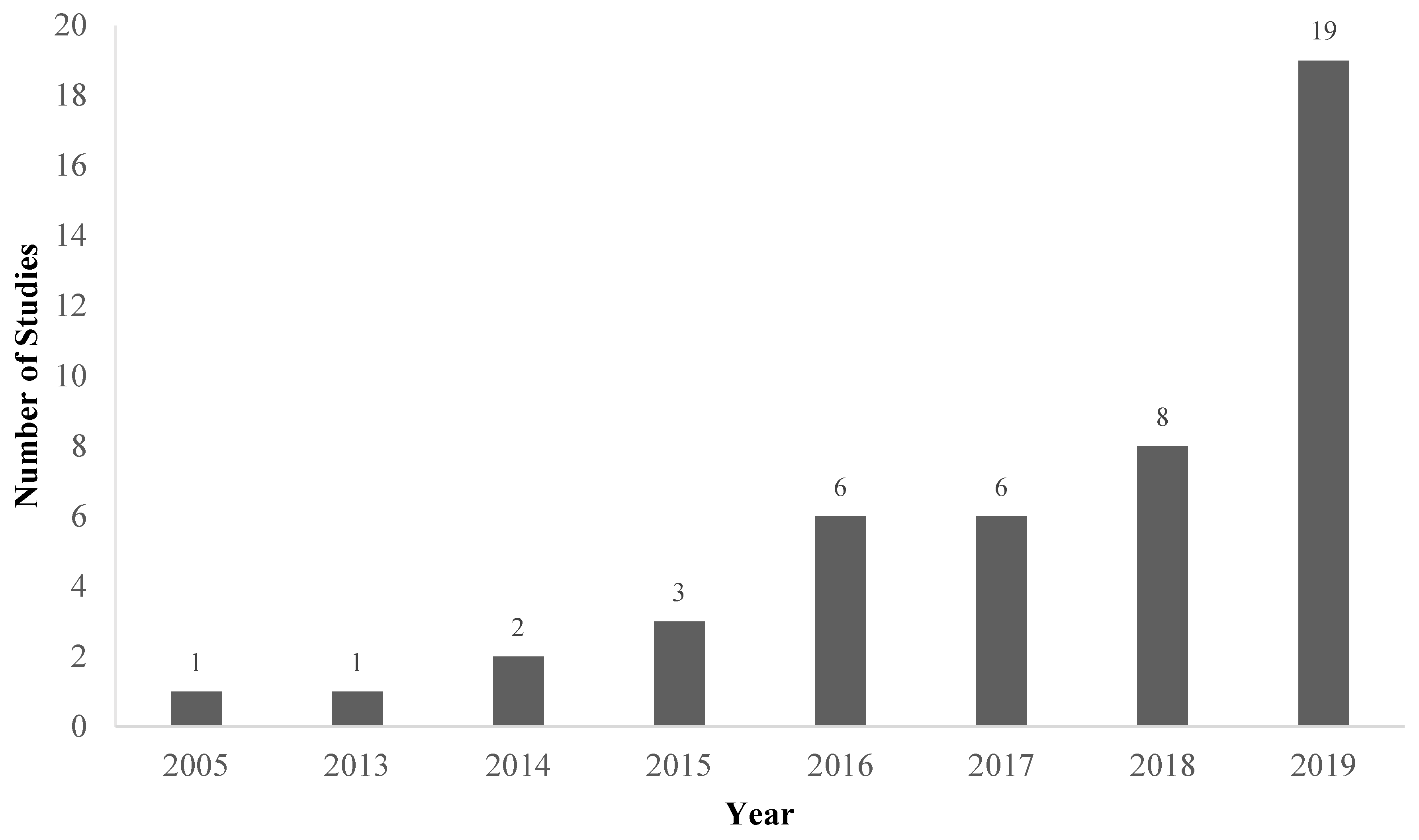
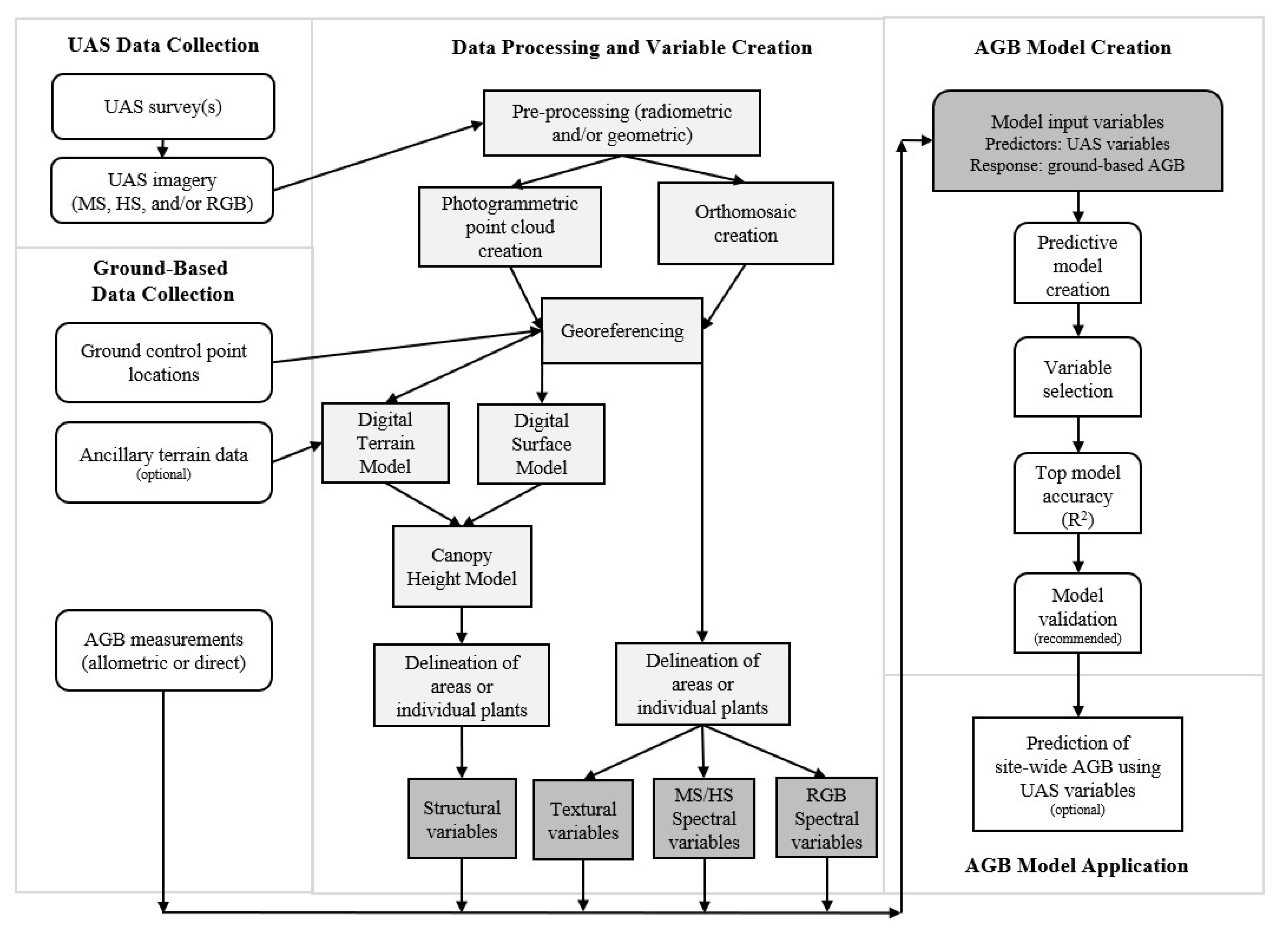
Table A1.
A summary of the 46 studies assembled for this review. Items recorded include study species and location, ground truth data type, UAS type, sensor type(s), flying height, photo overlap and sidelap, ground sample distance (GSD), whether analysis was done on an area-based plots or individual plants, spectral input data used, structural input data used, textural input data used, any other input data used, ground model source, best statistical model type, R2 of top calibration model and top variables.
| Study Parameters | Data Collection Parameters | Data Analysis Parameters | Results | ||||||||||||
|---|---|---|---|---|---|---|---|---|---|---|---|---|---|---|---|
| Species and Location | Ground Truth Data 1 | Sensor 2 | Flight Height | Overlap, Sidelap | GSD (cm/pixel) | Area Based? | Spectral Data | Structural Data | Texture Data | Other Data | Terrain Model Source | Best Statistical Method 3 | R2 | Top Variables | Study |
| Corn, alfalfa, soybean, USA | Direct measurements of dry biomass | RGB | 200 m | unknown | 10 cm | Area-based | NGRDI | n/a | n/a | n/a | n/a | SLR | 0.39–0.88 | NGRDI | [60] |
| Ryegrass crop, Japan | Direct measurements of dry biomass | 3-band MS | 100 m | 50% | 2 cm | Area-based | DN of each band | n/a | n/a | n/a | n/a | MLR | 0.84 | DN of R, G, NIR | [18] |
| Cover crop, USA | Direct measurements of dry biomass | 4-band MS | 100 m | 70%, 80% | 15 cm | Area-based | 4 indices | n/a | n/a | n/a | n/a | SLR | 0.92 | NDVI and GNDVI | [11] |
| Winter wheat crop, Germany | Direct measurements of dry biomass | 4-band MS | 25 m | 96%, 60% | 4 cm | Area-based | NDVI, REIP | n/a | n/a | n/a | n/a | SLR | 0.72–0.85 | NDVI, REIP | [24] |
| Wheat crop, China | Direct measurements of dry biomass | 2-band MS | 1 m | Unknown | <1 cm | Area-based | NDVI, RVI | n/a | n/a | n/a | n/a | SLR | 0.62–0.66 | RVI, NDVI | [58] |
| Wheat crop, Finland | Direct measurements of dry biomass | 42-band HS | 140 m | 78%, 67% | 20 cm | Area-based | All HS bands, NDVI | n/a | n/a | n/a | DTM from ALS data | KNN | 0.57–0.80 | All HS bands with correction | [61] |
| Rice crop, China | Direct measurements of dry biomass | 4-band MS | 80 m | 70% | 8 cm | Area-based | 10 spectral indices | n/a | n/a | n/a | n/a | LME | 0.75–0.89 | All VIs | [62] |
| Tallgrass prairie, USA | Direct measurements of dry biomass | 3-band MS | 5, 20, 50 m | Unknown | 1–9 cm | Area-based | NDVI | n/a | n/a | n/a | n/a | SLR | 0.86–0.94 | NDVI | [77] |
| Coastal wetland, USA | Direct measurements of fresh and dry biomass | 5-band MS | 90 m | 75% | 6.1 cm | Area-based | 6 spectral indices | n/a | n/a | n/a | n/a | SLR | 0.36–0.71 | NDVI | [43] |
| Winter wheat, China | Direct measurements of dry biomass | RGB | 50 m | Unknown | 1 cm | Area-based | 3 RGB bands, 6 RGB indices | n/a | 8 image textures | n/a | DTM interpolated from ground points | SWR, RF | 0.84 | All | [2] |
| Rice crop, China | Direct measurements of dry biomass | 6-band MS | 100 m | unknown | 5 cm | Area-based | 8 spectral indices | n/a | 8 textures, NDTIs | n/a | n/a | SWR | 0.86 | 2 texture, 1 RGB VI | [26] |
| Barley crop, Germany | Direct measurements of fresh and dry biomass | RGB | 50 m | >80% | <1 cm | Area-based | n/a | Mean height | n/a | n/a | Leaf-off DSM | SER | 0.81–0.82 | Mean height | [23] |
| Rice crop, Germany | Direct measurements of fresh and dry biomass | RGB | 7-10 m | 95% | <1 cm | Area-based | n/a | Mean plot height | n/a | n/a | DTM from interpolating plant-free point | SLR | 0.68–0.81 | Mean height | [74] |
| Black oat crop, Brazil | Direct measurements of fresh and dry biomass | RGB | 25 m | 90% | <2 cm | Area-based | n/a | Mean plot height | n/a | n/a | Leaf-off DTM | SER | 0.69–0.94 | Mean height | [75] |
| Temperate grasslands, Germany | Direct measurements of dry biomass | RGB | 20 m | 80% | <1 cm | Area-based | n/a | Mean plot height | n/a | n/a | DTM from raster ground point classification | RMAR | 0.62–0.81 | Mean height | [19] |
| Deciduous forest, USA | Allometric measurements of tree biomass | RGB | 80m | 80% | 3.4 cm | Area-based | n/a | Mean height | n/a | n/a | LiDAR DTM | SLR | 0.80 | Mean height | [55] |
| Coniferous forest, China | Allometric measurements of tree biomass | RGB | 400 m | 80%, 60% | 5 cm | Individual trees | n/a | Tree height | n/a | n/a | DTM from point cloud classification | SER | 0.98 | Max height | [1] |
| Pine tree plantation, Portugal | Allometric measurements of tree biomass | RGB | 170m | 80%, 75% | 6 cm | Individual trees | n/a | Tree height, crown area, diameter | n/a | n/a | DTM from point cloud classification | SER | 0.79–0.84 | All | [50] |
| Tropical forest, Costa Rica | Allometric measurements of tree biomass | RGB | 30–40 m | 90%, 75% | ~10 cm | Area-based | n/a | Canopy height, proportion, roughness, openness | n/a | n/a | DTMs from point cloud and ground-based GPS interpolation | SLR | 0.81–0.83 | Median height | [48] |
| Temperate grasslands, China | Direct measurements of dry biomass | RGB | 3m, 20m | 70% | ~ 1 cm | Area-based | n/a | 5 canopy height metrics | n/a | n/a | DTM from point cloud ground point classification | SLogR, SLR | 0.76–0.78 | Mean height, median height | [65] |
| Temperate grasslands, Germany | Direct measurements of fresh and dry biomass | RGB | 25 m | 80% | ~1 cm | Area-based | n/a | 10 canopy height metrics | n/a | n/a | DTM from TLS data | SLR | 0.0–0.62 | 75th percentile of height | [63] |
| Eggplant, tomato and cabbage crops, India | Direct measurements of fresh biomass | RGB | 20 m | 80% | <1 cm | Area-based | n/a | 14 canopy height metrics | n/a | n/a | DTM from point cloud ground point classification | RF | 0.88–0.95 | All | [34] |
| Mixed forest, Japan | Allometric measurements of tree biomass | RGB | 650 m | 85% | 14 cm | Area-based | n/a | 12 point cloud and 4 CHM metrics | n/a | n/a | LiDAR DTM | RF | 0.87–0.94 | 5 height metrics | [28] |
| Onion crop, Spain | Direct measurements of dry leaf and bulb biomass | RGB | 44 m | 60%, 40% | 1 cm | Area-based | n/a | 3 canopy height, volume and cover metrics | n/a | n/a | Bare-earth DTM | SER | 0.76–0.95 | Canopy volume | [22] |
| Rye and timothy pastures, Norway | Direct measurements of dry biomass | RGB | 30 m | 90%, 60% | <2 cm | Area-based | n/a | Mean plot volume | n/a | n/a | None | SLR | 0.54 | Volume | [64] |
| Boreal forest, Alaska | Allometric measurements of tree biomass | RGB | 100m | 90% | 1.9–2.7 cm | Individual tree crowns and plot level | n/a | Tree crown volume | n/a | n/a | DTM from point cloud classification | OLSR | 0.74–0.92 | Canopy volume | [8] |
| Tropical woodland, Malawi | Allometric measurements of tree biomass | RGB, 2-band MS | 286–487 m | 90%, 70–80% | 10–15 cm | Area-based | 15 RGB and 15 MS indices per 6 bands | 86 canopy height or canopy density features | n/a | n/a | DTM derived from point cloud ground point classification | MLR | 0.76 | 4 height metrics | [57] |
| Tropical forests, Myanmar | Allometric measurements of tree biomass | RGB | 91–96 m | 82% | <4 cm | Area-based | 4 RGB indices of spectral change | 11 height variables, 3 disturbed area variables | n/a | n/a | None | Type 1 Tobit | 0.77 | 2 height metrics | [49] |
| Tropical woodland, Malawi | Allometric measurements of biomass | RGB | 325 m | 80%, 90% | ~5 cm | Area-based | 15 spectral variables per RGB band | 15 canopy height metrics, 10 canopy density metrics | n/a | n/a | DTMs derived from ground point classification or SRTM data | MLR | 0.67 | 2 height, 1 spectral metric | [30] |
| Aquatic plants, China | Direct measurements of dry biomass | RGB | 50m | 60%, 80% | 10 cm | Area-based | 7 RGB indices | 3 height metrics | n/a | n/a | Winter DTM | SWR | 0.84 | 2 spectral, 3 height metrics | [9] |
| Cover crop, Switzerland | Direct measurements of dry biomass | RGB, 5-band MS | 50 m, 30 m | >75%, >65% | <10 cm | Area-based | 1 RGB index, 2 MS indices | Plant height and canopy cover | n/a | n/a | GPS measurements taken on the ground | SLR | 0.74 | 90th percentile of height | [21] |
| Rice crop, China | Direct measurements of dry biomass | RGB, 25-band MS | 25 m | 60%, 75% | 1–5 cm | Area-based | 9 spectral indices | Mean crop height | n/a | n/a | DTM from point cloud ground point classification | RF | 0.90 | Height, 7 RGB VIs, 3 MS VIs | [5] |
| Winter wheat, China | Direct measurements of dry biomass | RGB, 125-band HS | 50 m | 1–2.5 cm | Area-based | 3 RGB bands, 4 HS bands, 9 RGB indices, 8 HS indices | Crop height | n/a | n/a | DTM interpolated from manual ground point classification | RF | 0.96 | All RGB data | [20] | |
| Winter wheat, Germany | Direct measurements of fresh and dry biomass | RGB | 50 m | 60%, 60% | ~1 cm | Area-based | 5 spectral variables | Plant height, crop area | n/a | n/a | DTM from leaf-off flight | MLR | 0.70–0.94 | 2 principal components | [25] |
| Wheat crop, China | Direct measurements of dry biomass | RGB | 30 m | 80%, 60% | 1.66 cm | Area-based | 10 spectral indices | 8 height metrics | n/a | n/a | Leaf-off DTM | RF | 0.76 | All | [12] |
| Maize crop, China | Direct measurements of dry biomass | RGB, 4-band MS | 60 m | 80%, 75% | <1 cm | Area-based | 11 spectral indices | 3 canopy metrics | n/a | n/a | DTM interpolated from un-vegetated points | RF | 0.94 | 3 structural, 2 RGB VI, 1 MS VI metrics | [16] |
| Maize crop, China | Direct measurements of dry biomass | RGB | 150 m | 80%, 40% | 2 cm | Area-based | 8 spectral indices | 4 height metrics | n/a | n/a | DTM interpolated from ALS | RF | 0.78 | 3 structural, 2 RGB metrics | [15] |
| Maize crop, China | Direct measurements of fresh and dry biomass | RGB | 30 m | 90% | <1 cm | Area-based | 6 spectral variables | 6 canopy height variables | n/a | n/a | None | MLR | 0.85 | 3 RGB, 1 structural metric | [4] |
| Barley crop, Germany | Direct measurements of dry biomass | RGB | 50 m | Unknown | 1 cm | Area-based | 3 RGB indices | Mean crop height | n/a | VI*Height | Leaf-off DTM | MNLR | 0.84 | 1 structural, 1 spectral, 4 structural times spectral metrics | [66] |
| Poplar plantation, Spain | Allometric measurements of tree biomass | RGB, 5-band MS | 100 m | 80%, 60% | 4–6 cm | Individual trees | NDVI | Tree height | n/a | NDVI* Height | None | MLR | 0.54 | NDVI * Height | [67] |
| Winter wheat, China | Direct measurements of dry biomass | 125-band HS | 50 m | Unknown | 1 cm | Area-based | 5 HS bands, 14 HS VIs | Plant height | n/a | VI*Height | DTM interpolated from identified ground points | PLSR | 0.78 | 8 structural times spectral metrics | [6] |
| Grassland, Germany | Direct measurements of dry biomass | RGB | 13–16 m and 60 m | Unknown | 1–2 cm | Area-based | RGBVI | Mean plot height | n/a | GrassI (height + RGBVI* 0.25) | Leaf-off DTM | SLR | 0.64 | Mean plot height | [68] |
| Soybean crop, USA | Direct measurements of dry biomass | RGB | 30m | 90%, 90% | <1 cm | Area-based | 3 RGB bands, 17 RGB indices | 6 canopy height metrics, canopy volume | n/a | VI-weighted canopy volume | Winter DTM | SWR | 0.91 | All | [3] |
| Rice crop, China | Direct measurements of dry biomass | RGB, 12-band MS | 120 m | Unknown | 6.5 | Area-based | 11 MS indices + band reflectance of 12 bands | 17 TIN-derived metrics | n/a | Growing degree days (GDD) | Winter DTM | RF | 0.92 | All spectral, structural, GDD metrics | [13] |
| Ryegrass crop, Belgium | Direct measurements of dry biomass | RGB | 30 m | 80% | <2 cm | Area-based | 10 spectral indices | 7 canopy height metrics | n/a | GDD, ΔGDD between cuts | DTMs from interpolation of ground points and from leaf-off flights | MLR | 0.81 | 2 structural, 1 spectral, 2 GDD metrics | [69] |
| Maize crop, Belgium | Direct measurements of dry biomass | RGB | 50 m | 80% | ≤ 5 cm | Area-based | 5 spectral indices | Median plot height | n/a | Ground-based AGB estimate | LiDAR DTM | PLSR | 0.82 | All spectral metrics, mean height, field-measured AGB | [27] |
Direct measurements = destructive sampling; allometric measurements = non-destructive sampling. 2 RGB = visible light camera; MS = multispectral camera; HS = hyperspectral camera. 3 SLR = simple linear regression; SER = simple exponential regression; MLR = multiple linear regression; OLSR = ordinary least squares regression; RMAR = reduced major axis regression; SWR = stepwise regression; PLSR = partial least squares regression; RF = random forest; KNN = K Nearest Neighbor; SLogR = simple logarithmic regression; LME = linear mixed effects; MNLR = multiple non-linear regression.
References
- Lin, J.; Wang, M.; Ma, M.; Lin, Y. Aboveground Tree Biomass Estimation of Sparse Subalpine Coniferous Forest with UAV Oblique Photography. Remote Sens. 2018, 10, 1849. [Google Scholar] [CrossRef] [Green Version]
- Yue, J.; Yang, G.; Tian, Q.; Feng, H.; Xu, K.; Zhou, C. Estimate of winter-wheat above-ground biomass based on UAV ultrahigh- ground-resolution image textures and vegetation indices. ISPRS J. Photogramm. Remote Sens. 2019, 150, 226–244. [Google Scholar] [CrossRef]
- Maimaitijiang, M.; Sagan, V.; Sidike, P.; Maimaitiyiming, M.; Hartling, S.; Peterson, K.T.; Maw, M.J.W.; Shakoor, N.; Mockler, T.; Fritschi, F.B. Vegetation Index Weighted Canopy Volume Model (CVM VI) for soybean biomass estimation from Unmanned Aerial System-based RGB imagery. ISPRS J. Photogramm. Remote Sens. 2019, 151, 27–41. [Google Scholar] [CrossRef]
- Niu, Y.; Zhang, L.; Zhang, H.; Han, W.; Peng, X. Estimating Above-Ground Biomass of Maize Using Features Derived from UAV-Based RGB Imagery. Remote Sens. 2019, 11, 1261. [Google Scholar] [CrossRef] [Green Version]
- Cen, H.; Wan, L.; Zhu, J.; Li, Y.; Li, X.; Zhu, Y.; Weng, H.; Wu, W.; Yin, W.; Xu, C.; et al. Dynamic monitoring of biomass of rice under different nitrogen treatments using a lightweight UAV with dual image—Frame snapshot cameras. Plant Methods 2019, 15, 1–16. [Google Scholar] [CrossRef]
- Yue, J.; Yang, G.; Li, C.; Li, Z.; Wang, Y.; Feng, H.; Xu, B. Estimation of winter wheat above-ground biomass using unmanned aerial vehicle-based snapshot hyperspectral sensor and crop height improved models. Remote Sens. 2017, 9, 708. [Google Scholar] [CrossRef] [Green Version]
- Zhang, X.; Zhang, F.; Qi, Y.; Deng, L.; Wang, X.; Yang, S. New research methods for vegetation information extraction based on visible light remote sensing images from an unmanned aerial vehicle (UAV). Int. J. Appl. Earth Obs. Geoinf. 2019, 78, 215–226. [Google Scholar] [CrossRef]
- Alonzo, M.; Andersen, H.; Morton, D.C.; Cook, B.D. Quantifying Boreal Forest Structure and Composition Using UAV Structure from Motion. Forests 2018, 9, 119. [Google Scholar] [CrossRef] [Green Version]
- Jing, R.; Gong, Z.; Zhao, W.; Pu, R.; Deng, L. Above-bottom biomass retrieval of aquatic plants with regression models and SfM data acquired by a UAV platform—A case study in Wild Duck Lake Wetland, Beijing, China. ISPRS J. Photogramm. Remote Sens. 2017, 134, 122–134. [Google Scholar] [CrossRef]
- Maimaitijiang, M.; Ghulam, A.; Sidike, P.; Hartling, S.; Maimaitiyiming, M.; Peterson, K.; Shavers, E.; Fishman, J.; Peterson, J.; Kadam, S.; et al. Unmanned Aerial System (UAS)-based phenotyping of soybean using multi-sensor data fusion and extreme learning machine. ISPRS J. Photogramm. Remote Sens. 2017, 134, 43–58. [Google Scholar] [CrossRef]
- Yuan, M.; Burjel, J.C.; Isermann, J.; Goeser, N.J.; Pittelkow, C.M. Unmanned aerial vehicle–based assessment of cover crop biomass and nitrogen uptake variability. J. Soil Water Conserv. 2019, 74, 350–359. [Google Scholar] [CrossRef] [Green Version]
- Lu, N.; Zhou, J.; Han, Z.; Li, D.; Cao, Q.; Yao, X.; Tian, Y.; Zhu, Y.; Cao, W.; Cheng, T. Improved estimation of aboveground biomass in wheat from RGB imagery and point cloud data acquired with a low-cost unmanned aerial vehicle system. Plant Methods 2019, 15, 1–16. [Google Scholar] [CrossRef] [PubMed] [Green Version]
- Jiang, Q.; Fang, S.; Peng, Y.; Gong, Y.; Zhu, R.; Wu, X.; Ma, Y.; Duan, B.; Liu, J. UAV-Based Biomass Estimation for Rice-Combining Spectral, TIN-Based Structural and Meteorological Features. Remote Sens. 2019, 11, 890. [Google Scholar] [CrossRef] [Green Version]
- Viljanen, N.; Honkavaara, E. A Novel Machine Learning Method for Estimating Biomass of Grass Swards Using a Photogrammetric Canopy Height Model, Images and Vegetation Indices Captured by a Drone. Agriculture 2018, 8, 70. [Google Scholar] [CrossRef] [Green Version]
- Li, W.; Niu, Z.; Chen, H.; Li, D.; Wu, M.; Zhao, W. Remote estimation of canopy height and aboveground biomass of maize using high-resolution stereo images from a low-cost unmanned aerial vehicle system. Ecol. Indic. 2016, 67, 637–648. [Google Scholar] [CrossRef]
- Han, L.; Yang, G.; Dai, H.; Xu, B.; Yang, H.; Feng, H.; Li, Z.; Yang, X. Modeling maize above-ground biomass based on machine learning approaches using UAV remote-sensing data. Plant Methods 2019, 15, 1–19. [Google Scholar] [CrossRef] [Green Version]
- Näsi, R.; Viljanen, N.; Kaivosoja, J.; Alhonoja, K.; Hakala, T.; Markelin, L.; Honkavaara, E. Estimating Biomass and Nitrogen Amount of Barley and Grass Using UAV and Aircraft Based Spectral and. Remote Sens. 2018, 10, 1082. [Google Scholar] [CrossRef] [Green Version]
- Fan, X.; Kawamura, K.; Xuan, T.D.; Yuba, N.; Lim, J.; Yoshitoshi, R.; Minh, T.N.; Kurokawa, Y.; Obitsu, T. Low-cost visible and near-infrared camera on an unmanned aerial vehicle for assessing the herbage biomass and leaf area index in an Italian ryegrass field. Grassl. Sci. 2018, 64, 145–150. [Google Scholar] [CrossRef]
- Grüner, E.; Astor, T.; Wachendorf, M. Biomass Prediction of Heterogeneous Temperate Grasslands Using an SfM Approach Based on UAV Imaging. Agronomy 2019, 9, 54. [Google Scholar] [CrossRef] [Green Version]
- Yue, J.; Feng, H.; Jin, X.; Yuan, H.; Li, Z.; Zhou, C.; Yang, G.; Tian, Q. A Comparison of Crop Parameters Estimation Using Images from UAV-Mounted Snapshot Hyperspectral Sensor and High-Definition Digital Camera. Remote Sens. 2018, 10, 1138. [Google Scholar] [CrossRef] [Green Version]
- Roth, L.; Streit, B. Predicting cover crop biomass by lightweight UAS-based RGB and NIR photography: An applied photogrammetric approach. Precis. Agric. 2018, 19, 93–114. [Google Scholar] [CrossRef] [Green Version]
- Ballesteros, R.; Fernando, J.; David, O.; Moreno, M.A. Onion biomass monitoring using UAV - based RGB. Precis. Agric. 2018, 19, 840–857. [Google Scholar] [CrossRef]
- Bendig, J.; Bolten, A.; Bennertz, S.; Broscheit, J.; Eichfuss, S.; Bareth, G. Estimating Biomass of Barley Using Crop Surface Models (CSMs) Derived from UAV-Based RGB Imaging. Remote Sens. 2014, 6, 10395–10412. [Google Scholar] [CrossRef] [Green Version]
- Geipel, J.; Link, J.; Wirwahn, J.A.; Claupein, W. A Programmable Aerial Multispectral Camera System for In-Season Crop Biomass and Nitrogen Content Estimation. Agriculture 2016, 6, 4. [Google Scholar] [CrossRef] [Green Version]
- Schirrmann, M.; Giebel, A.; Gleiniger, F.; Pflanz, M.; Lentschke, J.; Dammer, K. Monitoring Agronomic Parameters of Winter Wheat Crops with Low-Cost UAV Imagery. Remote Sens. 2016, 8, 706. [Google Scholar] [CrossRef] [Green Version]
- Zheng, H.; Cheng, T.; Zhou, M.; Li, D.; Yao, X.; Tian, Y.; Cao, W.; Zhu, Y. Improved estimation of rice aboveground biomass combining textural and spectral analysis of UAV imagery. Precis. Agric. 2019, 20, 611–629. [Google Scholar] [CrossRef]
- Michez, A.; Bauwens, S.; Brostaux, Y.; Hiel, M.P.; Garré, S.; Lejeune, P.; Dumont, B. How far can consumer-grade UAV RGB imagery describe crop production? A 3D and multitemporal modeling approach applied to Zea mays. Remote Sens. 2018, 10, 1798. [Google Scholar] [CrossRef] [Green Version]
- Jayathunga, S.; Owari, T.; Tsuyuki, S. Digital Aerial Photogrammetry for Uneven-Aged Forest Management: Assessing the Potential to Reconstruct Canopy Structure and Estimate Living Biomass. Remote Sens. 2019, 11, 338. [Google Scholar] [CrossRef] [Green Version]
- Cunliffe, A.M.; Brazier, R.E.; Anderson, K. Ultra-fine grain landscape-scale quantification of dryland vegetation structure with drone-acquired structure-from-motion photogrammetry. Remote Sens. Environ. 2016, 183, 129–143. [Google Scholar] [CrossRef] [Green Version]
- Kachamba, D.J.; Ørka, H.O.; Gobakken, T.; Eid, T.; Mwase, W. Biomass Estimation Using 3D Data from Unmanned Aerial Vehicle Imagery in a Tropical Woodland. Remote Sens. 2016, 8, 968. [Google Scholar] [CrossRef] [Green Version]
- Zolkos, S.G.; Goetz, S.J.; Dubayah, R. A meta-analysis of terrestrial aboveground biomass estimation using lidar remote sensing. Remote Sens. Environ. 2013, 128, 289–298. [Google Scholar] [CrossRef]
- Zhao, F.; Guo, Q.; Kelly, M. Allometric equation choice impacts lidar-based forest biomass estimates: A case study from the Sierra National Forest, CA. Agric. For. Meteorol. 2012, 165, 64–72. [Google Scholar] [CrossRef]
- Li, F.; Zeng, Y.; Luo, J.; Ma, R.; Wu, B. Modeling grassland aboveground biomass using a pure vegetation index. Ecol. Indic. 2016, 62, 279–288. [Google Scholar] [CrossRef]
- Moeckel, T.; Dayananda, S.; Nidamanuri, R.R.; Nautiyal, S.; Hanumaiah, N.; Buerkert, A.; Wachendorf, M. Estimation of Vegetable Crop Parameter by Multi-temporal UAV-Borne Images. Remote Sens. 2018, 10, 805. [Google Scholar] [CrossRef] [Green Version]
- Moukomla, S.; Srestasathiern, P.; Siripon, S.; Wasuhiranyrith, R.; Kooha, P.; Moukomla, S. Estimating above ground biomass for eucalyptus plantation using data from unmanned aerial vehicle imagery. Proc. SPIE - Int. Soc. Opt. Eng. 2018, 10783, 1–13. [Google Scholar]
- Paul, K.I.; Radtke, P.J.; Roxburgh, S.H.; Larmour, J.; Waterworth, R.; Butler, D.; Brooksbank, K.; Ximenes, F. Validation of allometric biomass models: How to have confidence in the application of existing models. For. Ecol. Manag. 2018, 412, 70–79. [Google Scholar] [CrossRef]
- Roxburgh, S.H.; Paul, K.I.; Clifford, D.; England, J.R.; Raison, R. Guidelines for constructing allometric models for the prediction of woody biomass: How many individuals to harvest? Ecosphere 2015, 6, 1–27. [Google Scholar] [CrossRef] [Green Version]
- Seidel, D.; Fleck, S.; Leuschner, C. Review of ground-based methods to measure the distribution of biomass in forest canopies. Ann. For. Sci. 2011, 68, 225–244. [Google Scholar] [CrossRef] [Green Version]
- Dusseux, P.; Hubert-Moy, L.; Corpetti, T.; Vertès, F. Evaluation of SPOT imagery for the estimation of grassland biomass. Int. J. Appl. Earth Obs. Geoinf. 2015, 38, 72–77. [Google Scholar] [CrossRef]
- Eitel, J.U.H.; Magney, T.S.; Vierling, L.A.; Brown, T.T.; Huggins, D.R. LiDAR based biomass and crop nitrogen estimates for rapid, non-destructive assessment of wheat nitrogen status. Field Crop. Res. 2014, 159, 21–32. [Google Scholar] [CrossRef]
- Hansen, P.M.; Schjoerring, J.K. Reflectance measurement of canopy biomass and nitrogen status in wheat crops using normalized difference vegetation indices and partial least squares regression. Remote Sens. Environ. 2003, 86, 542–553. [Google Scholar] [CrossRef]
- Næsset, E.; Gobakken, T. Estimation of above- and below-ground biomass across regions of the boreal forest zone using airborne laser. Remote Sens. Environ. 2008, 112, 3079–3090. [Google Scholar] [CrossRef]
- Doughty, C.L.; Cavanaugh, K.C. Mapping Coastal Wetland Biomass from High Resolution Unmanned Aerial Vehicle (UAV) Imagery. Remote Sens. 2019, 11, 540. [Google Scholar] [CrossRef] [Green Version]
- Burnham, K.P.; Anderson, D.R. Multimodel inference: Understanding AIC and BIC in model selection. Sociol. Methods Res. 2004, 33, 261–304. [Google Scholar] [CrossRef]
- Shahbazi, M.; Théau, J.; Ménard, P. Recent applications of unmanned aerial imagery in natural resource management. GIScience Remote Sens. 2014, 51, 339–365. [Google Scholar] [CrossRef]
- Anderson, K.; Gaston, K.J. Lightweight unmanned aerial vehicles will revolutionize spatial ecology. Front. Ecol. Environ. 2013, 11, 138–146. [Google Scholar] [CrossRef] [Green Version]
- Jayathunga, S.; Owari, T.; Tsuyuki, S. The use of fixed–wing UAV photogrammetry with LiDAR DTM to estimate merchantable volume and carbon stock in living biomass over a mixed conifer–broadleaf forest. Int. J. Appl. Earth Obs. Geoinf. 2018, 73, 767–777. [Google Scholar] [CrossRef]
- Zahawi, R.A.; Dandois, J.P.; Holl, K.D.; Nadwodny, D.; Reid, J.L.; Ellis, E.C. Using lightweight unmanned aerial vehicles to monitor tropical forest recovery. Biol. Conserv. 2015, 186, 287–295. [Google Scholar] [CrossRef] [Green Version]
- Ota, T.; Ahmed, O.S.; Thu, S.; Cin, T.; Mizoue, N.; Yoshida, S. Estimating selective logging impacts on aboveground biomass in tropical forests using digital aerial photography obtained before and after a logging event from an unmanned aerial vehicle. For. Ecol. Manag. 2019, 433, 162–169. [Google Scholar] [CrossRef]
- Guerra-Hernández, J.; González-Ferreiro, E.; Monleón, V.J.; Faias, S.; Tomé, M.; Díaz-Varela, R. Use of Multi-Temporal UAV-Derived Imagery for Estimating Individual Tree Growth in Pinus pinea Stands. Forests 2017, 8, 300. [Google Scholar] [CrossRef]
- Salamí, E.; Barrado, C.; Pastor, E. UAV flight experiments applied to the remote sensing of vegetated areas. Remote Sens. 2014, 6, 11051–11081. [Google Scholar] [CrossRef] [Green Version]
- Laliberte, A.S.; Goforth, M.A.; Steele, C.M.; Rango, A. Multispectral remote sensing from unmanned aircraft: Image processing workflows and applications for rangeland environments. Remote Sens. 2011, 3, 2529–2551. [Google Scholar] [CrossRef] [Green Version]
- Deng, L.; Mao, Z.; Li, X.; Hu, Z.; Duan, F.; Yan, Y. UAV-based multispectral remote sensing for precision agriculture: A comparison between different cameras. ISPRS J. Photogramm. Remote Sens. 2018, 146, 124–136. [Google Scholar] [CrossRef]
- Maes, W.H.; Steppe, K. Perspectives for Remote Sensing with Unmanned Aerial Vehicles in Precision Agriculture. Trends Plant Sci. 2019, 24, 152–164. [Google Scholar] [CrossRef] [PubMed]
- Dandois, J.P.; Olano, M.; Ellis, E.C. Optimal altitude, overlap, and weather conditions for computer vision uav estimates of forest structure. Remote Sens. 2015, 7, 13895–13920. [Google Scholar] [CrossRef] [Green Version]
- Jensen, J.L.R.; Mathews, A.J. Assessment of Image-Based Point Cloud Products to Generate a Bare Earth Surface and Estimate Canopy Heights in a Woodland Ecosystem. Remote Sens. 2016, 8, 50. [Google Scholar] [CrossRef] [Green Version]
- Domingo, D.; Ørka, H.O.; Næsset, E.; Kachamba, D.; Gobakken, T. Effects of UAV Image Resolution, Camera Type, and Image Overlap on Accuracy of Biomass Predictions in a Tropical Woodland. Remote Sens. 2019, 11, 948. [Google Scholar] [CrossRef] [Green Version]
- Ni, W.; Dong, J.; Sun, G.; Zhang, Z.; Pang, Y.; Tian, X.; Li, Z.; Chen, E. Synthesis of Leaf-on and Leaf-off Unmanned Aerial Vehicle (UAV) Stereo Imagery for the Inventory of Aboveground Biomass of Deciduous Forests. Remote Sens. 2019, 11, 889. [Google Scholar] [CrossRef] [Green Version]
- Renaud, O.; Victoria-Feser, M.P. A robust coefficient of determination for regression. J. Stat. Plan. Inference 2010, 140, 1852–1862. [Google Scholar] [CrossRef] [Green Version]
- Hunt, E.R.; Cavigelli, M.; Daughtry, C.S.T.; McMurtrey, J.E.; Walthall, C.L. Evaluation of digital photography from model aircraft for remote sensing of crop biomass and nitrogen status. Precis. Agric. 2005, 6, 359–378. [Google Scholar] [CrossRef]
- Honkavaara, E.; Saari, H.; Kaivosoja, J.; Pölönen, I.; Hakala, T.; Litkey, P.; Mäkynen, J.; Pesonen, L. Processing and Assessment of Spectrometric, Stereoscopic Imagery Collected Using a Lightweight UAV Spectral Camera for Precision Agriculture. Remote Sens. 2013, 5, 5006–5039. [Google Scholar] [CrossRef] [Green Version]
- Wang, Y.; Zhang, K.; Tang, C.; Cao, Q.; Tian, Y.; Zhu, Y.; Cao, W.; Liu, X. Estimation of rice growth parameters based on linear mixed-effect model using multispectral images from fixed-wing unmanned aerial vehicles. Remote Sens. 2019, 11, 1371. [Google Scholar] [CrossRef] [Green Version]
- Wijesingha, J.; Moeckel, T.; Hensgen, F.; Wachendorf, M. Evaluation of 3D point cloud-based models for the prediction of grassland biomass. Int. J. Appl. Earth Obs. Geoinf. 2019, 78, 352–359. [Google Scholar] [CrossRef]
- Rueda-Ayala, V.P.; Peña, J.M.; Höglind, M.; Bengochea-Guevara, J.M.; Andújar, D. Comparing UAV-based technologies and RGB-D reconstruction methods for plant height and biomass monitoring on grass ley. Sensors 2019, 19, 535. [Google Scholar] [CrossRef] [PubMed] [Green Version]
- Zhang, H.; Sun, Y.; Chang, L.; Qin, Y.; Chen, J.; Qin, Y.; Du, J.; Yi, S.; Wan, Y. Estimation of Grassland Canopy Height and Aboveground Biomass at the Quadrat Scale Using Unmanned Aerial Vehicle. Remote Sens. 2018, 10, 851. [Google Scholar] [CrossRef] [Green Version]
- Bendig, J.; Yu, K.; Aasen, H.; Bolten, A.; Bennertz, S.; Broscheit, J.; Gnyp, M.L.; Bareth, G. Combining UAV-based plant height from crop surface models, visible, and near infrared vegetation indices for biomass monitoring in barley. Int. J. Appl. Earth Obs. Geoinf. 2015, 39, 79–87. [Google Scholar] [CrossRef]
- Peña, J.M.; De Castro, A.I.; Torres-sánchez, J.; Andújar, D.; San Martin, C.; Dorado, J.; Fernández-Quintanilla, C.; López-Granados, F. Estimating tree height and biomass of a poplar plantation with image-based UAV technology. Agric. Food 2018, 3, 313–326. [Google Scholar] [CrossRef]
- Possoch, M.; Bieker, S.; Hoffmeister, D.; Bolten, A.A.; Schellberg, J.; Bareth, G. Multi-Temporal crop surface models combined with the rgb vegetation index from UAV-based images for forage monitoring in grassland. Int. Arch. Photogramm. Remote Sens. Spat. Inf. Sci. - ISPRS Arch. 2016, XLI-B1, 991–998. [Google Scholar] [CrossRef]
- Borra-Serrano, I.; De Swaef, T.; Muylle, H.; Nuyttens, D.; Vangeyte, J.; Mertens, K.; Saeys, W.; Somers, B.; Roldán-Ruiz, I.; Lootens, P. Canopy height measurements and non-destructive biomass estimation of Lolium perenne swards using UAV imagery. Grass Forage Sci. 2019, 356–369. [Google Scholar] [CrossRef]
- Tucker, C.J. Red and photographic infrared linear combinations for monitoring vegetation. Remote Sens. Environ. 1979, 8, 127–150. [Google Scholar] [CrossRef] [Green Version]
- Mutanga, O.; Skidmore, A.K. Narrow band vegetation indices overcome the saturation problem in biomass estimation. Int. J. Remote Sens. 2004, 25, 3999–4014. [Google Scholar] [CrossRef]
- Rasmussen, J.; Ntakos, G.; Nielsen, J.; Svensgaard, J.; Poulsen, R.N.; Christensen, S. Are vegetation indices derived from consumer-grade cameras mounted on UAVs sufficiently reliable for assessing experimental plots? Eur. J. Agron. 2016, 74, 75–92. [Google Scholar] [CrossRef]
- Haralick, R.; Shanmugam, K.; Dinstein, I. Textural Features for Image Classification. IEEE Trans. Syst. Man. Cybern. 1973, SMC-3, 610–621. [Google Scholar] [CrossRef] [Green Version]
- Willkomm, M.; Bolten, A.; Bareth, G. Non-destructive monitoring of rice by hyperspectral in-field spectrometry and UAV-based remote sensing: Case study of field-grown rice in North Rhine-Westphalia, Germany. Int. Arch. Photogramm. Remote Sens. Spat. Inf. Sci. - ISPRS Arch. 2016, XLI-B1, 1071–1077. [Google Scholar] [CrossRef]
- Acorsi, M.G.; das Abati Miranda, F.D.; Martello, M.; Smaniotto, D.A.; Sartor, L.R. Estimating biomass of black oat using UAV-based RGB imaging. Agronomy 2019, 9, 344. [Google Scholar] [CrossRef] [Green Version]
- Ni, J.; Yao, L.; Zhang, J.; Cao, W.; Zhu, Y.; Tai, X. Development of an unmanned aerial vehicle-borne crop-growth monitoring system. Sensors 2017, 17, 502. [Google Scholar] [CrossRef] [Green Version]
- Wang, C.; Price, K.P.; Van Der Merwe, D.; An, N.; Wang, H. Modeling Above-Ground Biomass in Tallgrass Prairie Using Ultra-High Spatial Resolution sUAS Imagery. Photogramm. Eng. Remote Sens. 2014, 80, 1151–1159. [Google Scholar] [CrossRef]
- Wang, F.; Wang, F.; Zhang, Y.; Hu, J.; Huang, J. Rice Yield Estimation Using Parcel-Level Relative Spectral Variables from UAV-Based Hyperspectral Imagery. Front. Plant Sci. 2019, 10, 453. [Google Scholar] [CrossRef] [Green Version]
- Mulla, D.J. Twenty five years of remote sensing in precision agriculture: Key advances and remaining knowledge gaps. Biosyst. Eng. 2013, 114, 358–371. [Google Scholar] [CrossRef]
- Kelcey, J.; Lucieer, A. Sensor correction of a 6-band multispectral imaging sensor for UAV remote sensing. Remote Sens. 2012, 4, 1462–1493. [Google Scholar] [CrossRef] [Green Version]
- McGwire, K.C.; Weltz, M.A.; Finzel, J.A.; Morris, C.E.; Fenstermaker, L.F.; McGraw, D.S. Multiscale assessment of green leaf cover in a semi-arid rangeland with a small unmanned aerial vehicle. Int. J. Remote Sens. 2013, 34, 1615–1632. [Google Scholar] [CrossRef]
- Whitehead, K.; Hugenholtz, C.H. Remote sensing of the environment with small unmanned aircraft systems (UASs), part 1: A review of progress and challenges. J. Unmanned Veh. Syst. 2014, 02, 69–85. [Google Scholar] [CrossRef]
- Lebourgeois, V.; Bégué, A.; Labbé, S.; Mallavan, B.; Prévot, L.; Roux, B. Can commercial digital cameras be used as multispectral sensors? A crop monitoring test. Sensors 2008, 8, 7300–7322. [Google Scholar] [CrossRef] [PubMed]
- Calderón, R.; Navas-Cortés, J.A.; Lucena, C.; Zarco-Tejada, P.J. High-resolution airborne hyperspectral and thermal imagery for early detection of Verticillium wilt of olive using fluorescence, temperature and narrow-band spectral indices. Remote Sens. Environ. 2013, 139, 231–245. [Google Scholar] [CrossRef]
- James, M.R.; Robson, S.; Smith, M.W. 3-D uncertainty-based topographic change detection with structure-from-motion photogrammetry: Precision maps for ground control and directly georeferenced surveys. Earth Surf. Process. Landf. 2017, 1788, 1769–1788. [Google Scholar] [CrossRef]
- James, M.R.; Robson, S. Mitigating systematic error in topographic models derived from UAV and ground-based image networks. Earth Surf. Process. Landf. 2014, 39, 1413–1420. [Google Scholar] [CrossRef] [Green Version]
- Lisein, J.; Pierrot-Deseilligny, M.; Bonnet, S.; Lejeune, P. A photogrammetric workflow for the creation of a forest canopy height model from small unmanned aerial system imagery. Forests 2013, 4, 922–944. [Google Scholar] [CrossRef] [Green Version]
- Fonstad, M.A.; Dietrich, J.T.; Courville, B.C.; Jensen, J.L.; Carbonneau, P.E. Topographic structure from motion: A new development in photogrammetric measurement. Earth Surf. Process. Landf. 2013, 38, 421–430. [Google Scholar] [CrossRef] [Green Version]
- Hardin, P.; Jensen, R. Small-scale unmanned aerial vehicles in environmental remote sensing: Challenges and opportunities. GIScience Remote Sens. 2011, 48, 99–111. [Google Scholar] [CrossRef]
- Rahman, M.M.; McDermid, G.J.; Mckeeman, T.; Lovitt, J. A workflow to minimize shadows in UAV-based orthomosaics. J. Unmanned Veh. Syst. 2019, 7, 107–117. [Google Scholar] [CrossRef]
- Goodbody, T.R.H.; Coops, N.C.; Hermosilla, T.; Tompalski, P.; Pelletier, G. Vegetation Phenology Driving Error Variation in Digital Aerial Photogrammetrically Derived Terrain Models. Remote Sens. 2018, 10, 1554. [Google Scholar] [CrossRef] [Green Version]
- Gitelson, A.A.; Kaufman, Y.J.; Stark, R.; Rundquist, D. Novel algorithms for remote estimation of vegetation fraction. Remote Sens. Environ. 2002, 80, 76–87. [Google Scholar] [CrossRef] [Green Version]
- Assmann, J.J.; Kerby, J.T.; Cunliffe, A.M.; Myers-Smith, I.H. Vegetation monitoring using multispectral sensors—Best practices and lessons learned from high latitudes. J. Unmanned Veh. Syst. 2019, 7, 54–75. [Google Scholar] [CrossRef] [Green Version]
- Von Bueren, S.K.; Burkart, A.; Hueni, A.; Rascher, U.; Tuohy, M.P.; Yule, I.J. Deploying four optical UAV-based sensors over grassland: Challenges and limitations. Biogeosciences 2015, 12, 163–175. [Google Scholar] [CrossRef] [Green Version]
- Turner, D.; Lucieer, A.; Watson, C. An automated technique for generating georectified mosaics from ultra-high resolution Unmanned Aerial Vehicle (UAV) imagery, based on Structure from Motion (SFM) point clouds. Remote Sens. 2012, 4, 1392–1410. [Google Scholar] [CrossRef] [Green Version]
- Lowe, D.G. Distinctive image features from scale-invariant keypoints. Int. J. Comput. Vis. 2004, 60, 91–110. [Google Scholar] [CrossRef]
- Dandois, J.P.; Ellis, E.C. High spatial resolution three-dimensional mapping of vegetation spectral dynamics using computer vision. Remote Sens. Environ. 2013, 136, 259–276. [Google Scholar] [CrossRef] [Green Version]
- Ota, T.; Ogawa, M.; Mizoue, N.; Fukumoto, K.; Yoshida, S. Forest Structure Estimation from a UAV-Based Photogrammetric Point Cloud in Managed Temperate Coniferous Forests. Forests 2017, 8, 343. [Google Scholar] [CrossRef]
- Fraser, R.H.; Olthof, I.; Lantz, T.C.; Schmitt, C. UAV photogrammetry for mapping vegetation in the low-Arctic. Arct. Sci. 2016, 2, 79–102. [Google Scholar] [CrossRef] [Green Version]
- Reykdal, Ó. Drying and Storing of Harvested Grain: A Review of Methods. 2018. Available online: https://www.matis.is/media/matis/utgafa/05-18-Drying-and-storage-of-grain.pdf (accessed on 14 September 2019).
- Ogle, S.M.; Breidt, F.J.; Paustian, K. Agricultural Management Impacts on Soil Organic Carbon Storage under Moist and Dry Climatic Conditions of Temperate and Tropical Regions. Biogeo 2005, 72, 87–121. [Google Scholar] [CrossRef]
- Chen, D.; Huang, X.; Zhang, S.; Sun, X. Biomass modeling of larch (Larix spp.) plantations in China based on the mixed model, dummy variable model, and Bayesian hierarchical model. Forests 2017, 8, 268. [Google Scholar] [CrossRef] [Green Version]
Figure 1.
Number of peer-reviewed studies published per year using unmanned aerial system-borne passive sensors to estimate vegetation biomass. Total number (as of 31 August 2019) of papers published on the topic and fitting the requirements of this review = 46.
Figure 1.
Number of peer-reviewed studies published per year using unmanned aerial system-borne passive sensors to estimate vegetation biomass. Total number (as of 31 August 2019) of papers published on the topic and fitting the requirements of this review = 46.

Figure 2.
A schematic diagram of common steps used by studies summarized in this review for estimating the aboveground biomass (AGB) of vegetation using unmanned aerial system (UAS) data. Data collection steps are shown in rounded white rectangles; data processing in light grey rectangles; UAS-derived input data in dark grey rectangles; AGB model creation steps in white rectangles with rounded top corners; and model application in a white rectangle.

Table 1.
Structural information derived from UAS data that was used to model vegetation biomass in at least one study included in this review. Structural metrics could be calculated using individual plant or area-based approaches.
Table 1.
Structural information derived from UAS data that was used to model vegetation biomass in at least one study included in this review. Structural metrics could be calculated using individual plant or area-based approaches.
| Type | Variable | Used by |
|---|---|---|
| Height | Mean height | [3,9,12,13,15,16,19,20,21,23,25,28,30,34,48,49,50,57,58,63,65,67,68,69,74,75,76] |
| Maximum height | [1,3,4,13,28,30,34,48,57,63,65,69] | |
| Minimum height | [3,28,34,48,57,63,65,69] | |
| Median height | [12,21,27,48,63,65,69] | |
| Mode of height | [57] | |
| Count of height | [63] | |
| Standard deviation of height | [3,9,12,13,15,28,30,34,48,57,63,65,69] | |
| Coefficient of variation of height | [3,9,12,13,15,28,30,34,48,57,69] | |
| Variance of height | [57] | |
| Skewness of height | [30,34,57] | |
| Kurtosis of height | [30,34,57] | |
| Entropy of height | [13] | |
| Relief of height | [13,34] | |
| Height percentile(s) | [4,13,15,21,30,34,49,57,63,69] | |
| Area & Density | Canopy point density | [28,30,57] |
| Proportion of points > mean height relative to total number of points | [28,57] | |
| Proportion of points > mode height relative to total number of points | [57] | |
| Crown/vegetation area (canopy cover) | [3,21,50] | |
| Canopy relief ratio | [16,57] | |
| Crown isle—proportion of site where canopy has height greater than 2/3 of the 99th percentile of all heights | [48] | |
| Canopy openness—proportion of site area <2 m in height | [48] | |
| Canopy roughness—average of SD of each pixel from mean CHM | [48] | |
| Volume | Canopy/crown volume | [3,8,16,22,25,64] |
| VI-weighted canopy volume | [3] | |
| Change-based | Amount of change in DSM before and after plant removal | [49] |
| Other | Height*Spectral (various indices) | [6,66,67] |
| GrassI (RGBVI + CHM) | [68] | |
| TIN-based structure, area, slope | [13] |
Table 2.
All multispectral or hyperspectral vegetation indices used to model vegetation biomass in at least one of the studies included in this review. R, G, B and near infrared (NIR) indicate the measured reflectance (digital numbers) in red, green, blue and near-infrared wavelength ranges, respectively. Λ is used to indicate the reflectance at the given specific wavelength.
| Index | Formula | Used by |
|---|---|---|
| NDSI | (λ1 − λ2)/(λ2 + λ2) where 1 and 2 are any bands | [5] |
| MNDSI | (λ1 − λ2)/(λ1 − λ2) where 1, 2 and 3 are any bands | [5] |
| SR | (λ1/λ2) where 1 and 2 are any bands | [5,25] |
| NDVI | (NIR − R)/(NIR + R) | [6,11,13,16,20,26,43,61,67,76,77,78] |
| GNDVI | (NIR − G)/(NIR + G) | [13,16,26,43,62] |
| NDRE | (λ800 − λ720)/(λ800 + λ720) | [13,16,43,62] |
| SR | λ800/λ700 | [13] |
| NPCI | (λ670 − λ460)/(λ670 + λ460) | [20] |
| TVI | 0.5 * [120 * (λ800 − λ550) − 200 * (λ670 − λ550) | [6,11,13] |
| EVI | 2.5 * (λ800 − λ670)/(λ800 + 6 * λ670 − 7.5 * λ490 + 1) | [6,13,43] |
| EVI2 | 2.5 * (λ800 − λ680)/(λ800 + 2.4 * λ680 + 1) | [6,20] |
| GI | λ550/λ680 | [6] |
| RDVI | (λ798 − λ670)/sqrt(λ798 + λ670) | [13] |
| CI red edge | (λ780 − Λ710) − 1 OR (NIR/RE) − 1 | [13,16,26,43,62] |
| CI green | (λ780 − λ550) − 1 OR (NIR/green) − 1 | [13,16,43] |
| DATT | (λ800 − λ720)/(λ800 − λ680) | [26] |
| LCI | (λ850 − λ710)/(λ850 − λ680) | [13,20] |
| MCARI | [(λ700 − λ670) − 0.2(λ700 − λ550)] * (λ700/λ670) | [13,20] |
| MCARI1 | 1.2(2.5(λ790 − λ660) − 1.3(λ790 − λ560)) | [62] |
| SPVI | 0.4 * (3.7(λ800 − λ670) − 1.2 * |λ530 − λ670|) | [20] |
| OSAVI | 1.16(λ800 − λ670)/(λ800 + λ670 + 0.16) | [6,20,26,62] |
| REIP | 700 + 40 * (((λ667 + λ782)/2) − λ702)/(λ738 − λ702)) | [21,24] |
| MTVI | 1.2[1.2(λ800 − λ550) − (2.5(λ670 − λ550)] | [6,62] |
| MTVI2 | 1.5[1.2(λ800 − λ550) − 2.5(λ670 − λ550)]/sqrt[(2 * λ800 + 1)2 − (6 * λ800 − (5 * λ670)1/2) − 0.5]1/2 | [6,26,62] |
| RVI | λ800/λ670 | [6,16] |
| DVI1-3 | λ800 − λ680; λ750 − λ680; λ550 − λ680 | [6] |
| WDRVI | (0.1 * λ800 − λ680)/(0.1 * λ800 + λ680) | [6,16] |
| CVI | NIR * (R/G2) | [16] |
| BGI | λ460/λ560 | [20] |
| DATT | (λ790 − λ735)/(λ790 − λ660) | [62] |
| MSAVI | (2 * λ800 + 1 − sqrt(2 * λ800 + 1)2) − 8 * (λ800 − λ670) | [6,62] |
Table 3.
All RGB vegetation indices used at least once in vegetation biomass estimation models by studies included in this review. R, G, B and NIR indicate the measured reflectance (digital numbers) in red, green, blue and near-infrared wavelength ranges, respectively.
Table 3.
All RGB vegetation indices used at least once in vegetation biomass estimation models by studies included in this review. R, G, B and NIR indicate the measured reflectance (digital numbers) in red, green, blue and near-infrared wavelength ranges, respectively.
| Index | Formula1 | Used by |
|---|---|---|
| GRVI/NGRDI | (G − R)/(G + R) | [2,3,4,5,9,11,12,16,20,21,26,27,33,60] |
| ExG | 2 × G − R − B | [3,4,9,12,15,16,25,69] |
| GLA/GLI/VDVI | (2 * G − R − B)/(2 * G + R + B) | [3,5,9,12,15,16] |
| MGRVI | G2 − R2/G2 + R2 | [5,12] |
| ExB | 1.4 * B − G/(G + R + B) | [3,12] |
| ExR | 1.4 × R − B or 1.4 * (R − G)/(G + R + B) | [12,15] |
| ExGR | ExG index − ExR index | [3,4,9,12,15,69] |
| Red Ratio | R/(R + G + B) | [2,3,20] |
| Blue Ratio | B/(R + G + B) | [2,3,20] |
| Green Ratio | G/(R + G + B) | [2,3,20] |
| VARI | (G − R)/(G + R − B) | [2,3,5,12,16,20,26,27] |
| ExR | 1.4 * (R − G) | [2,3,20] |
| NRBI | (R − B)/(R + B) | [27] |
| NGBI | (G − B)/(G + B) | [27] |
| VEG | G/(RaB(1−a)) where a = 0.667 | [3,4,5,9,15] |
| WI | (G − B)/(R − G) | [3,15] |
| CIVE | 0.441 * R − 0.881 * G + 0.385 * B + 18.78745 | [3,4,9,15] |
| COM | 0.25 * ExG + 0.3 * ExGR + 0.33 * CIVE + 0.12 * VEG | [3,4,9,15] |
| TGI | G − (0.39 * R) − (0.61 * B) | [27] |
| RGBVI | (G2 − B * R)/(G2 + B * R) | [12,68] |
| IKAW | (R − B)/(R + B) | [3,12] |
| GRRI | G/R | [3,5] |
| GBRI | G/B | [3] |
| RBRI | R/B | [3] |
| BRRI | B/R | [20] |
| BGRI | B/G | [20] |
| RGRI | R/G | [20] |
| INT | (R + G + B)/3 | [3] |
| NDI | (red ratio index − green ratio index)/ (red ratio index + green ratio index + 0.01) | [3] |
| MVARI | (G − B)/(B + R − B) | [5] |
| IPCA | 0.994 * |R − B| + 0.961 * |G − B| + 0.914 * |G − R| | [3] |
| Δ Reflectance | Change in reflectance measured at two time periods | [49] |
© 2020 by the authors. Licensee MDPI, Basel, Switzerland. This article is an open access article distributed under the terms and conditions of the Creative Commons Attribution (CC BY) license (http://creativecommons.org/licenses/by/4.0/).
Share and Cite
MDPI and ACS Style
G. Poley, L.; J. McDermid, G. A Systematic Review of the Factors Influencing the Estimation of Vegetation Aboveground Biomass Using Unmanned Aerial Systems. Remote Sens. 2020, 12, 1052. https://doi.org/10.3390/rs12071052
AMA Style
G. Poley L, J. McDermid G. A Systematic Review of the Factors Influencing the Estimation of Vegetation Aboveground Biomass Using Unmanned Aerial Systems. Remote Sensing. 2020; 12(7):1052. https://doi.org/10.3390/rs12071052
Chicago/Turabian StyleG. Poley, Lucy, and Gregory J. McDermid. 2020. "A Systematic Review of the Factors Influencing the Estimation of Vegetation Aboveground Biomass Using Unmanned Aerial Systems" Remote Sensing 12, no. 7: 1052. https://doi.org/10.3390/rs12071052
Note that from the first issue of 2016, this journal uses article numbers instead of page numbers. See further details here.