60 Years of Glacier Elevation and Mass Changes in the Maipo River Basin, Central Andes of Chile

 , ,
, ,  , , ,
, , ,
Abstract
:1. Introduction
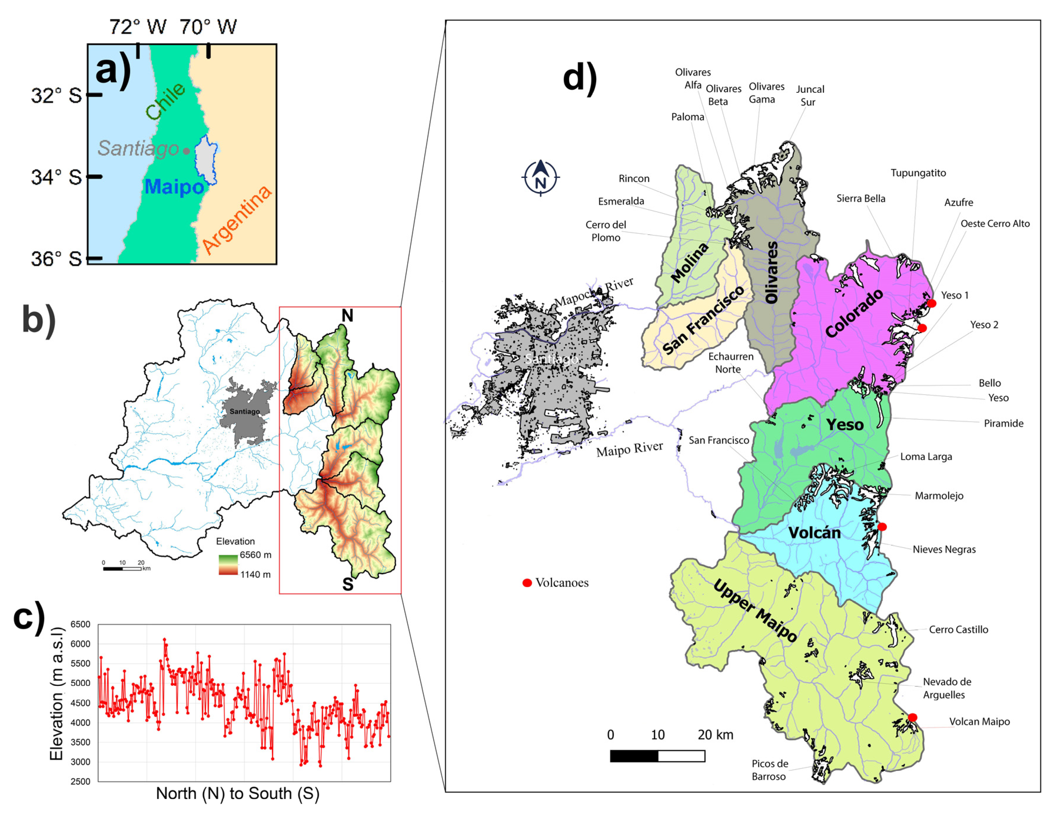
2. Study Area
3. Materials and Methods
3.1. Glacier Outlines
3.2. Glacier Elevation and Mass Changes
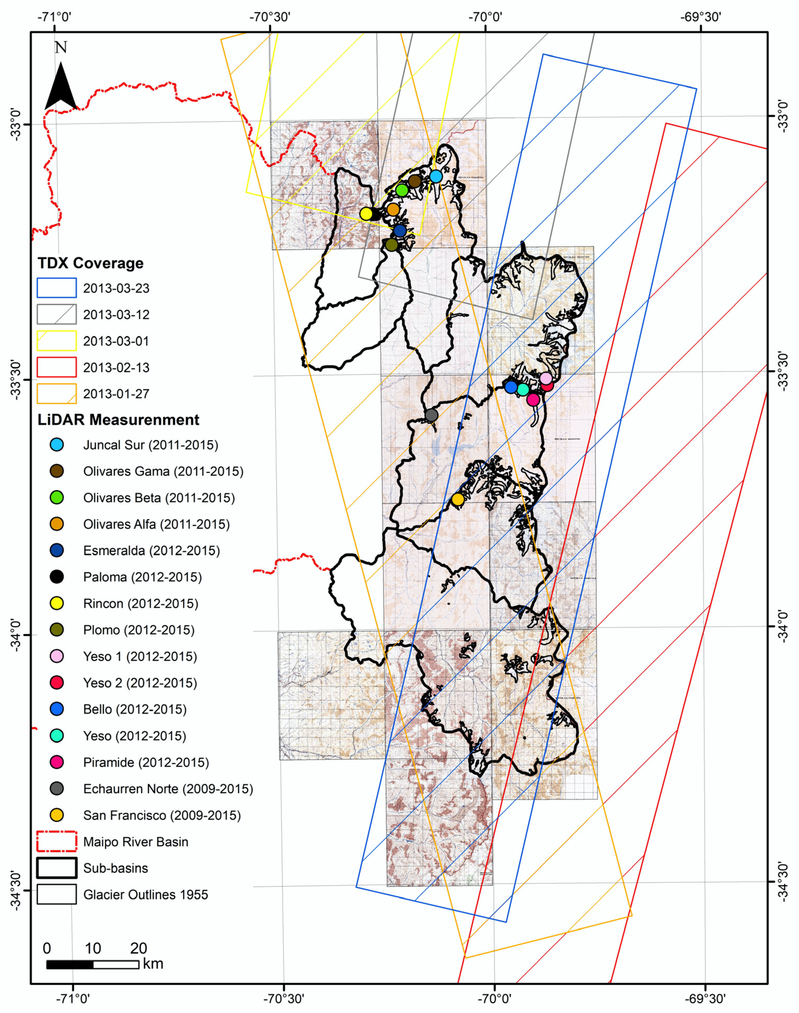
3.3. LiDAR Measurements
3.4. Uncertainties and Error Assessment
4. Results
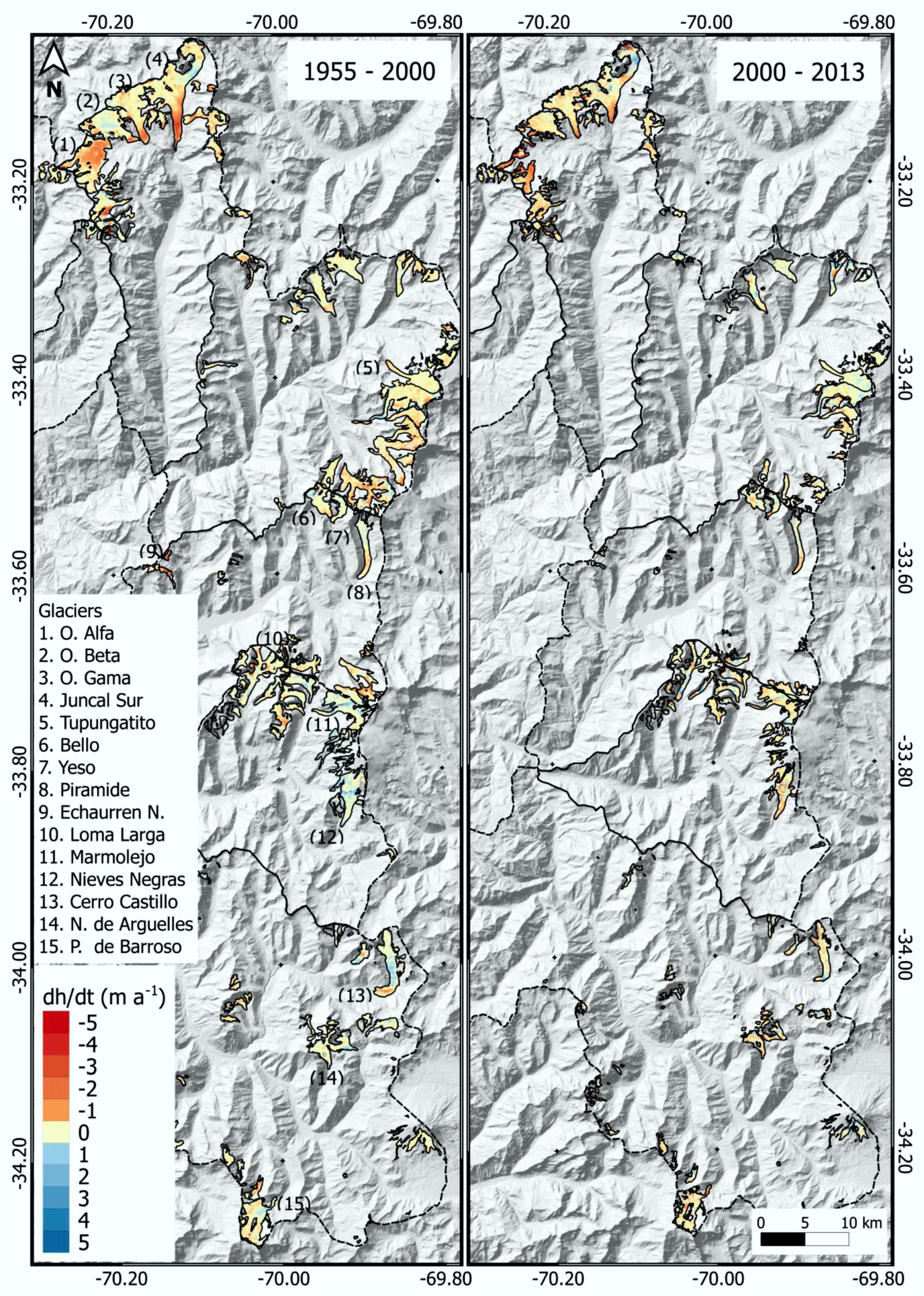
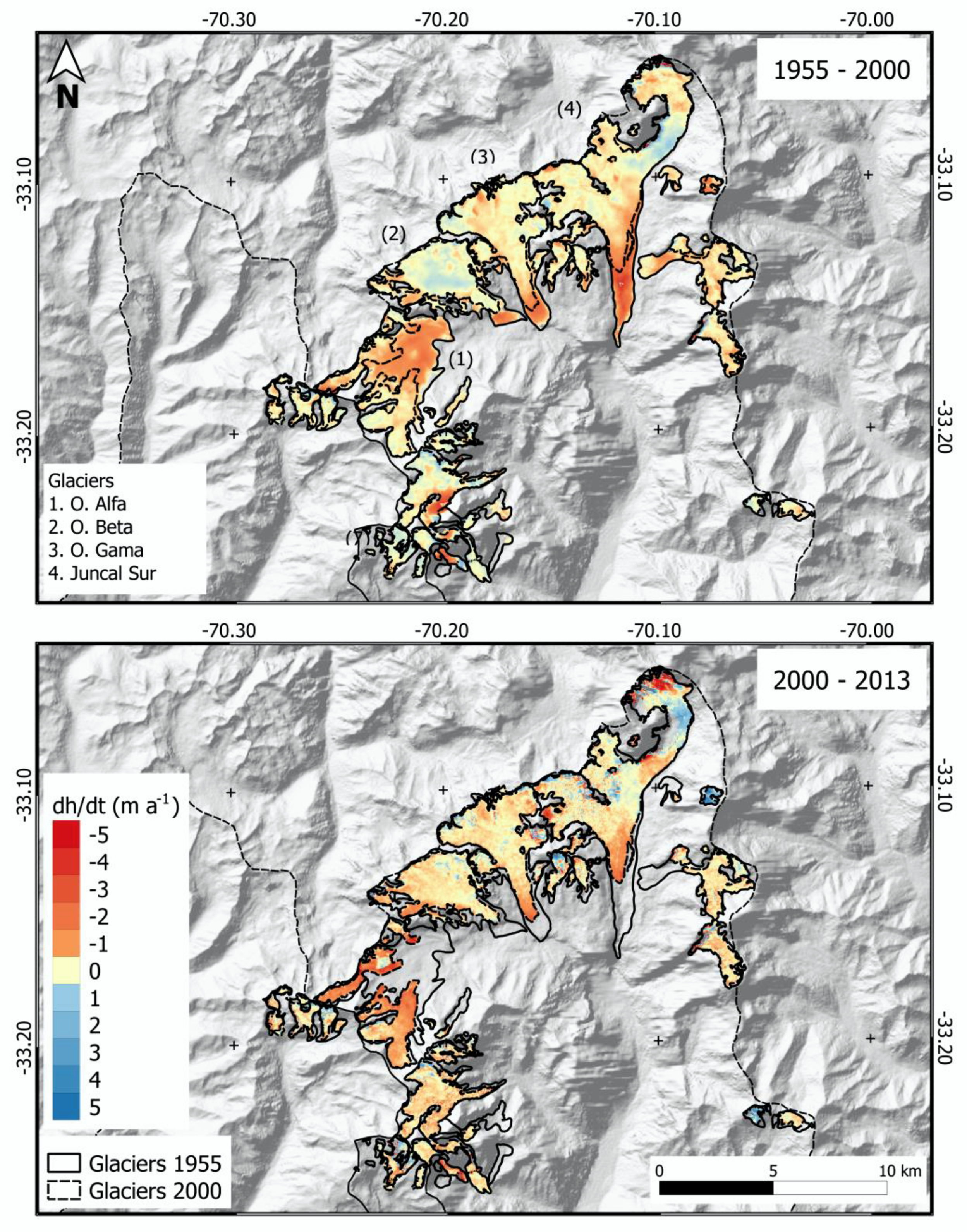
4.1. Glacier Elevation and Mass Changes from Satellite Products
4.2. Glacier Elevation Changes with LiDAR
5. Discussion
6. Conclusions
Supplementary Materials
Author Contributions
Funding
Acknowledgments
Conflicts of Interest
References
- Cogley, J.G.; Hock, R.; Rasmussen, L.A.; Arendt, A.A.; Bauder, A.; Braithwaite, R.J.; Jansson, P.; Kaser, G.; Möller, M.; Nicholson, L. Glossary of Glacier Mass Balance and Related Terms; IHP-VII Technical Documents in Hydrology No. 86, IACS Contribution No. 2; UNESCO-IHP: Paris, France, 2011. [Google Scholar]
- Hock, R.; Rasul, G.; Adler, C.; Cáceres, B.; Gruber, S.; Hirabayashi, Y.; Jackson, M.; Kääb, A.; Kang, S.; Kutuzov, S.; et al. High Mountain Areas. In IPCC Special Report on Ocean and the Cryosphere in a Changing Climate (SROCC); IPCC: Geneva, Switzerland, 2019. [Google Scholar]
- Huss, M.; Hock, R. A new model for global glacier change and sea-level rise. Front. Earth Sci. 2015, 3, 54. [Google Scholar] [CrossRef] [Green Version]
- Braun, M.H.; Malz, P.; Sommer, C.; Farías Barahona, D.; Sauter, T.; Casassa, G.; Soruco, A.; Skvarca, P.; Seehaus, T.C. Constraining glacier elevation and mass changes in South America. Nat. Clim. Chang. 2019, 9, 131–136. [Google Scholar] [CrossRef]
- Zemp, M.; Huss, M.; Thibert, E.; Eckert, N.; McNabb, R.; Huber, J.; Barandun, M.; Machguth, H.; Nussbaumer, S.U.; Gärtner-Roer, I.; et al. Global glacier mass changes and their contributions to sea-level rise from 1961 to 2016. Nature 2019, 568, 382–386. [Google Scholar] [CrossRef] [PubMed]
- Bamber, J.L.; Rivera, A. A review of remote sensing methods for glacier mass balance determination. Glob. Planet. Chang. 2007, 59, 138–148. [Google Scholar] [CrossRef]
- Fischer, M.; Huss, M.; Kummert, M.; Hoelzle, M. Application and validation of long-range terrestrial laser scanning to monitor the mass balance of very small glaciers in the Swiss Alps. Cryosphere 2016, 10, 1279–1295. [Google Scholar] [CrossRef] [Green Version]
- Mölg, N.; Bolch, T. Structure-from-Motion Using Historical Aerial Images to Analyse Changes in Glacier Surface Elevation. Remote Sens. 2017, 9, 1021. [Google Scholar] [CrossRef] [Green Version]
- Berthier, E.; Vincent, C.; Magnússon, E.; Gunnlaugsson, Á.Þ.; Pitte, P.; Le Meur, E.; Masiokas, M.; Ruiz, L.; Pálsson, F.; Belart, J.M.C.; et al. Glacier topography and elevation changes derived from Pléiades sub-meter stereo images. Cryosphere 2014, 8, 2275–2291. [Google Scholar] [CrossRef] [Green Version]
- Dussaillant, I.; Berthier, E.; Brun, F.; Masiokas, M.; Hugonnet, R.; Favier, V.; Rabatel, A.; Pitte, P.; Ruiz, P. Two decades of glacier mass loss along the Andes. Nat. Geosci. 2019, 12, 802–808. [Google Scholar] [CrossRef]
- Rivera, A.; Casassa, G.; Acuña, C.; Lange, H. Variaciones recientes de glaciares en Chile. Investig. Geogr. 2000, 34, 29–60. [Google Scholar] [CrossRef] [Green Version]
- Casassa, G.; Rivera, A.; Schwikowski, M. Glacier mass-balance data for southern South America (30°S–56°S). In Glacier Science and Environmental Change; Knight, P., Ed.; Blackwell Science Ltd.: Hoboken, NJ, USA, 2006; pp. 239–241. [Google Scholar]
- Zemp, M.; Frey, H.; Gärtner-Roer, I.; Nussbaumer, S.U.; Hoelzle, M.; Paul, F.; Haeberli, W.; Denzinger, F.; Ahlstrøm, A.P.; Anderson, B.; et al. Historically unprecedented global glacier decline in the early 21st century. J. Glaciol. 2015, 61, 745–762. [Google Scholar] [CrossRef] [Green Version]
- Malmros, J.K.; Mernild, S.H.; Wilson, R.; Fensholt, R.; Yde, J.C. Glacier area changes in the central Chilean and Argentinean Andes 1955–2013/2014. J. Glaciol. 2016, 62, 391–401. [Google Scholar] [CrossRef] [Green Version]
- Carrasco, J.; Casassa, G.; Quintana, J. Changes of the 0 °C isotherm in central Chile during the last quarter of the XXth Century. Hydrol. Sci. J. 2005, 50, 933–948. [Google Scholar] [CrossRef]
- Pellicciotti, F.; Burlando, P.; Van Vliet, K. Recent trends in precipitation and streamflow in the Aconcagua River Basin, central Chile. In Glacier Mass Balance Changes and Meltwater Discharge (Selected Papers from Sessions at the IAHS Assembly in Foz do Iguaçu, Brazil, 2005); IAHS Publ.: Wallingford, Oxfordshire, UK, 2007; p. 318. [Google Scholar]
- Falvey, M.; Garreaud, R. Regional cooling in a warming world: Recent temperature trends in the southeast Pacific and along the west coast of subtropical South America (1979–2006). J. Geophys. Res. 2009, 114, D04102. [Google Scholar] [CrossRef]
- Boisier, J.P.; Rondanelli, R.; Garreaud, R.; Muñoz, F. Anthropogenic and natural contributions to the Southeast Pacific precipitation decline and recent megadrought in Central Chile. Geophys. Res. Lett. 2016, 43, 413–421. [Google Scholar] [CrossRef] [Green Version]
- Garreaud, R.; Alvarez-Garreton, C.; Barichivich, J.; Boisier, J.P.; Christie, D.; Galleguillos, M.; LeQuesne, C.; McPhee, J.; Zambrano-Bigiarini, M. The 2010–2015 mega drought in Central Chile: Impacts on regional hydroclimate and vegetation. Hydrol. Earth Syst. Sci. 2017, 21, 6307–6327. [Google Scholar] [CrossRef] [Green Version]
- Burger, F.; Ayala, A.; Farías, D.; Shaw, T.; MacDonell, S.; Brock, B.; McPhee, J.; Pelliciotti, F. Interannual variability in glacier contribution to runoff from a high-elevation Andean catchment: Understanding the role of debris cover in glacier hydrology. Hydrol. Process 2019, 33, 214–229. [Google Scholar] [CrossRef] [Green Version]
- Escobar, F.; Casassa, G.; Pozo, V. Variaciones de un glaciar de montaña en los Andes de Chile central en las últimas dos décadas. Bull. Inst. Fr. Etudes Andin. 1995, 24, 683–695. [Google Scholar]
- Masiokas, M.H.; Christie, D.A.; Le Quesne, C.; Pitte, P.; Ruiz, L.; Villalba, R.; Luckman, B.H.; Berthier, E.; Nussbaumer, S.U.; González-Reyes, A.; et al. Reconstructing the annual mass balance of the Echaurren Norte glacier (Central Andes, 33.5, S) using local and regional hydroclimatic data. Cryosphere 2016, 10, 927–940. [Google Scholar] [CrossRef] [Green Version]
- Farías-Barahona, D.; Vivero, S.; Casassa, G.; Schaefer, M.; Burger, F.; Seehaus, T.; Iribarren-Anacona, P.; Escobar, F.; Braun, M.H. Geodetic mass balances and area changes of Echaurren Norte Glacier (Central Andes, Chile) between 1955 and 2015. Remote Sens. 2019, 11, 260. [Google Scholar] [CrossRef] [Green Version]
- Falaschi, D.; Lenzano, M.G.; Tadono, T.; Vich, A.I.; Lenzano, L.E. Balance de masa geodésico 2000–2011 de los glaciares de la cuenca del río Atuel, Andes Centrales de Mendoza (Argentina). Geoacta 2018, 42, 7–22. [Google Scholar]
- Garreaud, R.; Boisier, J.P.; Rondanelli, R.; Montecinos, A.; Sepúlveda, H.; Veloso-Águila, D. The Central Chile Mega Drought (2010–2018): A Climate dynamics perspective. Int. J. Climatol. 2020, 40, 421–439. [Google Scholar] [CrossRef]
- Ayala, A.; Pellicciotti, F.; MacDonell, S.; McPhee, J.; Vivero, S.; Campos, C.; Egli, P. Modelling the hydrological response of debris-free and debris-covered glaciers to present climatic conditions in the semiarid Andes of central Chile. Hydrol. Process 2016, 30, 4036–4058. [Google Scholar] [CrossRef]
- Bravo, C.; Loriaux, T.; Rivera, A.; Brock, B.W. Assessing glacier melt contribution to streamflow at Universidad Glacier, central Andes of Chile. Hydrol. Earth Syst. Sci. 2017, 21, 3249–3266. [Google Scholar] [CrossRef] [Green Version]
- Montecinos, A.; Aceituno, P. Seasonality of the ENSO-related rainfall variability in central Chile and associated circulation anomalies. J. Clim. 2003, 16, 281–296. [Google Scholar] [CrossRef] [Green Version]
- Viale, M.; Garreaud, R. Orographic effects of the subtropical and extratropical Andes on upwind precipitating clouds. J. Geophys. Res. 2015, 120, 4962–4974. [Google Scholar] [CrossRef]
- Garreaud, R. Warm winter storms in Central Chile. J. Hydrometeorol. 2013, 14, 1515–1534. [Google Scholar] [CrossRef]
- Viale, M.; Garreaud, R. Summer precipitation events over the western slope of the subtropical Andes. Mon. Wea. Rev. 2014, 142, 1074–1092. [Google Scholar] [CrossRef]
- Masiokas, M.H.; Villalba, R.; Luckman, B.H.; Le Quesne, C.; Aravena, J.C. Snowpack variations in the central Andes of Argentina and Chile, 1951–2005: Large-scale atmospheric influences and implications for water resources in the region. J. Clim. 2006, 19, 6334–6352. [Google Scholar] [CrossRef]
- Barcaza, G.; Nussbaumer, S.; Tapia, G.; Valdés, J.; García, J.; Videla, Y.; Albornoz, A.; Arias, V. Glacier inventory and recent glacier variations in the Andes of Chile, South America. Ann. Glaciol. 2017, 58, 1–15. [Google Scholar] [CrossRef] [Green Version]
- Marangunic, C. Inventario de Glaciares. Hoya del río Maipo. Dirección General de Aguas, Publicación G-2, Santiago. Technical Report 1979. Available online: www.dga.cl (accessed on 13 April 2020).
- Mikhail, E.M.; Bethel, J.S.; McGlone, J.C. Introduction to Modern Photogrammetry; John Wiley and Sons Inc.: New York, NY, USA, 2001. [Google Scholar]
- Lliboutry, L. Nieves y Glaciares de Chile: Fundamentos de Glaciologia, Ediciones de la Universidad de Chile 1956; Universidad de Chile: Santiago, RM, Chile, 1956. [Google Scholar]
- Paul, F.; Huggel, C.; Kääb, A. Combining satellite multispectral image data and a digital elevation model for mapping debris-covered glaciers. Remote Sens. Environ. 2004, 89, 510–518. [Google Scholar] [CrossRef]
- Farr, T.G.; Rosen, P.; Caro, E.; Crippen, R.; Duren, R.; Hensley, S.; Kobrick, M.; Paller, M.; Rodriguez, E.; Roth, L.; et al. The Shuttle Radar Topography Mission. Rev. Geophys. 2007, 45, RG2004. [Google Scholar] [CrossRef] [Green Version]
- Krieger, G.; Moreira, A.; Fiedler, H.; Hajnsek, I.; Werner, M.; Younis, M.; Zink, M. TanDEM-X: A satellite formation for high-resolution SAR interferometry. IEEE Trans. Geosci. Remote Sens. 2007, 45, 3317–3341. [Google Scholar] [CrossRef] [Green Version]
- Seehaus, T.; Malz, P.; Sommer, C.; Lippl, S.; Cochachin, A.; Braun, M. Changes of the tropical glaciers throughout Peru between 2000 and 2016 – mass balance and area fluctuations. Cryosphere 2019, 13, 2537–2556. [Google Scholar] [CrossRef] [Green Version]
- Vijay, S.; Braun, M.H. Elevation Change Rates of Glaciers in the Lahaul-Spiti (Western Himalaya, India) during 2000–2012 and 2012–2013. Remote Sens. 2016, 8, 1038. [Google Scholar] [CrossRef] [Green Version]
- Goldstein, R.M.; Werner, C.L. Radar interferogram filtering for geophysical applications. Geophys. Res. Lett. 1998, 25, 4035–4038. [Google Scholar] [CrossRef] [Green Version]
- Costantini, M. A novel phase unwrapping method based on network programming. IEEE Trans. Geosci. Remote Sens. 1998, 36, 813–821. [Google Scholar] [CrossRef]
- Nuth, C.; Kääb, A. Co-registration and bias corrections of satellite elevation data sets for quantifying glacier thickness change. Cryosphere 2011, 5, 271–290. [Google Scholar] [CrossRef] [Green Version]
- Malz, P.; Meier, E.; Casassa, G.; Jaña, R.; Skvarca, P.; Braun, M. Elevation and mass changes of the Southern Patagonia Icefield derived from TanDEM-X and SRTM data. Remote Sens. 2018, 10, 188. [Google Scholar] [CrossRef] [Green Version]
- Farías-Barahona, D.; Sommer, C.; Sauter, T.; Bannister, D.; Seehaus, T.; Malz, P.; Casassa, G.; Mayewski, P.A.; Turton, J.V.; Braun, M.H. Detailed quantification of glacier elevation and mass changes in South Georgia. Environ. Res. Lett. 2020, 15, 034036. [Google Scholar] [CrossRef]
- Huss, M. Density assumptions for converting geodetic glacier volume change to mass change. Cryosphere 2013, 7, 877–887. [Google Scholar] [CrossRef] [Green Version]
- DGA. Levantamiento Topográfico Láser Aerotransportado para los Glaciares Echaurren Norte y San Francisco; Technical Report; Terra Remote Sensing Inc.: Sidney, BC, Canada, 2009. [Google Scholar]
- DGA. Levantamiento Láser Aerotransportado de los Glaciares Cipreses, Cortaderal y Palomo, Cuenca del río Cachapoal, Zona Central, Chile; Technical Report; Terra Remote Sensing Inc.: Sidney, BC, Canada, 2011. [Google Scholar]
- DGA. Modelo Digital de Elevación de Centros Montañosos y Glaciares de las Zonas Glaciológicas Norte y Centro, Mediante LiDAR Aerotranpsortado; Technical Report; Digimapas: Santiago, Chile, 2015. [Google Scholar]
- Paul, F.; Barrand, N.E.; Baumann, S.; Berthier, E.; Bolch, T.; Casey, K.; Frey, H.; Joshi, S.P.; Konovalov, V.; Bris, R.L. On the accuracy of glacier outlines derived from remote-sensing data. Ann. Glaciol. 2013, 54, 171–182. [Google Scholar] [CrossRef] [Green Version]
- Rolstad, C.; Haug, T.; Denby, B. Spatially integrated geodetic glacier mass balance and its uncertainty based on geostatistical analysis: Application to the western Svartisen ice cap, Norway. J. Glaciol. 2009, 55, 666–680. [Google Scholar] [CrossRef] [Green Version]
- Dussaillant, I.; Berthier, E.; Brun, F. Geodetic Mass Balance of the Northern Patagonian Icefield from 2000 to 2012 Using Two Independent Methods. Front. Earth Sci. 2018, 6, 8. [Google Scholar] [CrossRef] [Green Version]
- Falaschi, D.; Bolch, T.; Rastner, P.; Lenzano, M.G.; Lenzano, L.; Lo Vecchio, A.; Moragues, S. Mass changes of alpine glaciers at the eastern margin of the Northern and Southern Patagonian Icefields between 2000 and 2012. J. Glaciol. 2017, 63, 258–272. [Google Scholar] [CrossRef] [Green Version]
- Rignot, E.; Rivera, A.; Casassa, G. Contribution of the Patagonia Icefields of South America to Sea Level Rise. Science 2003, 302, 434–437. [Google Scholar] [CrossRef] [PubMed] [Green Version]
- Rivera, A.; Benham, T.; Casassa, G.; Bamber, J.; Dowdeswell, J.A. Ice elevation and areal changes of glaciers from the Northern Patagonia Icefield, Chile. Glob. Planet. Chang. 2007, 59, 126–137. [Google Scholar] [CrossRef]
- Bown, F.; Rivera, A.; Acuña, C. Recent glacier variations at the Aconcagua basin, central Chilean Andes. Ann. Glaciol. 2008, 48, 43–48. [Google Scholar] [CrossRef] [Green Version]
- Rabatel, A.; Castebrunet, H.; Favier, V.; Nicholson, L.; Kinnard, C. Glacier changes in the Pascua-Lama region, Chilean Andes (29° S): Recent mass balance and 50 yr surface area variations. Cryosphere 2011, 5, 1029–1041. [Google Scholar] [CrossRef] [Green Version]
- Jacques-Coper, M.; Garreaud, R. Characterization of the 1970s climate shift in South America. Int. J. Climatol. 2014, 35, 2164–2179. [Google Scholar] [CrossRef]
- González-Reyes, Á.; McPhee, J.; Christie, D.A.; Le Quesne, C.; Szejner, P.; Masiokas, M.H.; Villalba, R.; Muñoz, A.A.; Crespo, S. Spatiotemporal Variations in Hydroclimate across the Mediterranean Andes (30°–37° S) since the Early Twentieth Century. J. Hydrometeorol. 2017, 18, 1929–1942. [Google Scholar] [CrossRef]
- Burger, F.; Brock, B.; Montecinos, A. Seasonal and elevation contrasts in temperature trends in Central Chile between 1979 and 2015. Glob. Planet. Chang. 2018, 162, 136–147. [Google Scholar] [CrossRef]
- Wouters, B.; Gardner, A.S.; Moholdt, G. Global glacier mass loss during the GRACE Satellite Mission (2002–2016). Front. Earth Sci. 2019, 7, 96. [Google Scholar] [CrossRef] [Green Version]
- Barcaza, G.; Segovia, A.; Farías, D.; Huenante, J.; Varela, B.; Gonzalez, D.; Vergara, A. Surface elevation change of Andean glaciers in Central Chile, based upon airborne laser altimetry and ground-truth GPS measurements. In Proceedings of the 26th International Union Geodesy and Geophysics, Prague, Czech Republic, 22 June–2 July 2015. [Google Scholar]
- Geoestudios, S.A. Implementación Nivel 2 Estrategia Nacional de Glaciares: Mediciones Glaciológicas Terrestres en Chile Central, Zona Sur y Patagonia. S.I.T. 327; Dirección General de Aguas: Santiago, Chile, 2013. [Google Scholar]
- Hernández, J.; Paredes, P.; Carrion, D.; Rivera, A. Ice elevation changes surveyed with Airborne laser scanning data. In Proceedings of the First IEEE International Symposium of Geoscience and Remote Sensing (GRSS-CHILE), Valdivia, Chile, 15–16 June 2017. [Google Scholar] [CrossRef]
- Reid, T.; Brock, B. Assessing ice-cliff backwasting and its contribution to total ablation of debris-covered Miage glacier, Mont Blanc massif, Italy. J. Glaciol. 2014, 60, 3–13. [Google Scholar] [CrossRef] [Green Version]
- Brun, F.; Wagnon, P.; Berthier, E.; Shea, J.M.; Immerzeel, W.W.; Kraaijenbrink, P.D.A.; Vincent, C.; Reverchon, C.; Shrestha, D.; Arnaud, Y. Ice cliff contribution to the tongue-wide ablation of Changri Nup Glacier, Nepal, central Himalaya. Cryosphere 2018, 12, 3439–3457. [Google Scholar] [CrossRef] [Green Version]
- Rankl, M.; Braun, M. Glacier elevation and mass changes over the central Karakoram region estimated from TanDEM-X and SRTM/X-SAR digital elevation models. Ann. Glaciol. 2016, 51, 273–281. [Google Scholar] [CrossRef] [Green Version]
- Milana, J.P. A model of the Glaciar Horcones Inferior surge, Aconcagua region, Argentina. J. Glaciol. 2007, 53, 565–572. [Google Scholar] [CrossRef] [Green Version]
- Pitte, P.; Berthier, E.; Masiokas, M.H.; Cabot, V.; Ruiz, L.; Ferri Hidalgo, L.; Gargantini, H.; Zalazar, L. Geometric evolution of the Horcones Inferior Glacier (Mount Aconcagua, Central Andes) during the 2002–2006 surge: Horcones Inferior Glacier Surge. J. Geophys. Res. 2016, 121, 111–127. [Google Scholar] [CrossRef] [Green Version]
- Bruce, R.H.; Cabrera, G.; Leiva, J.C.; Lenzano, L. The 1985 surge and ice dam of Glaciar Grande del Nevado del Plomo, Argentina. J. Glaciol. 1987, 33, 131–132. [Google Scholar] [CrossRef] [Green Version]
- Espizua, L.E.; Bengochea, J.D. Surge of Grande del Nevado glacier (Mendoza, Argentina) in 1984: Its evolution through satellite images. Geogr. Ann. 1990, 72, 255–259. [Google Scholar] [CrossRef]
- Peña, H.; Klohn, W. Hidrología de desastres en Chile: Crecidas catastróficas recientes de origen meterológicos. Rev. de la Soc. Chil. de Ing. Hidraúlica 1990, 5, 21–38. [Google Scholar]
- Falaschi, D.; Bolch, T.; Lenzano, G.; Tadono, T.; Lo Vecchio, A.; Lenzano, L. New evidence of glacier surges in the Central Andes of Argentina and Chile. Progr. Phys. Geogr. 2018, 42, 792–825. [Google Scholar] [CrossRef]


| Glaciers (North to South) | Sub-Basin | Date 1 | Date 2 | Total Coverage (%) |
|---|---|---|---|---|
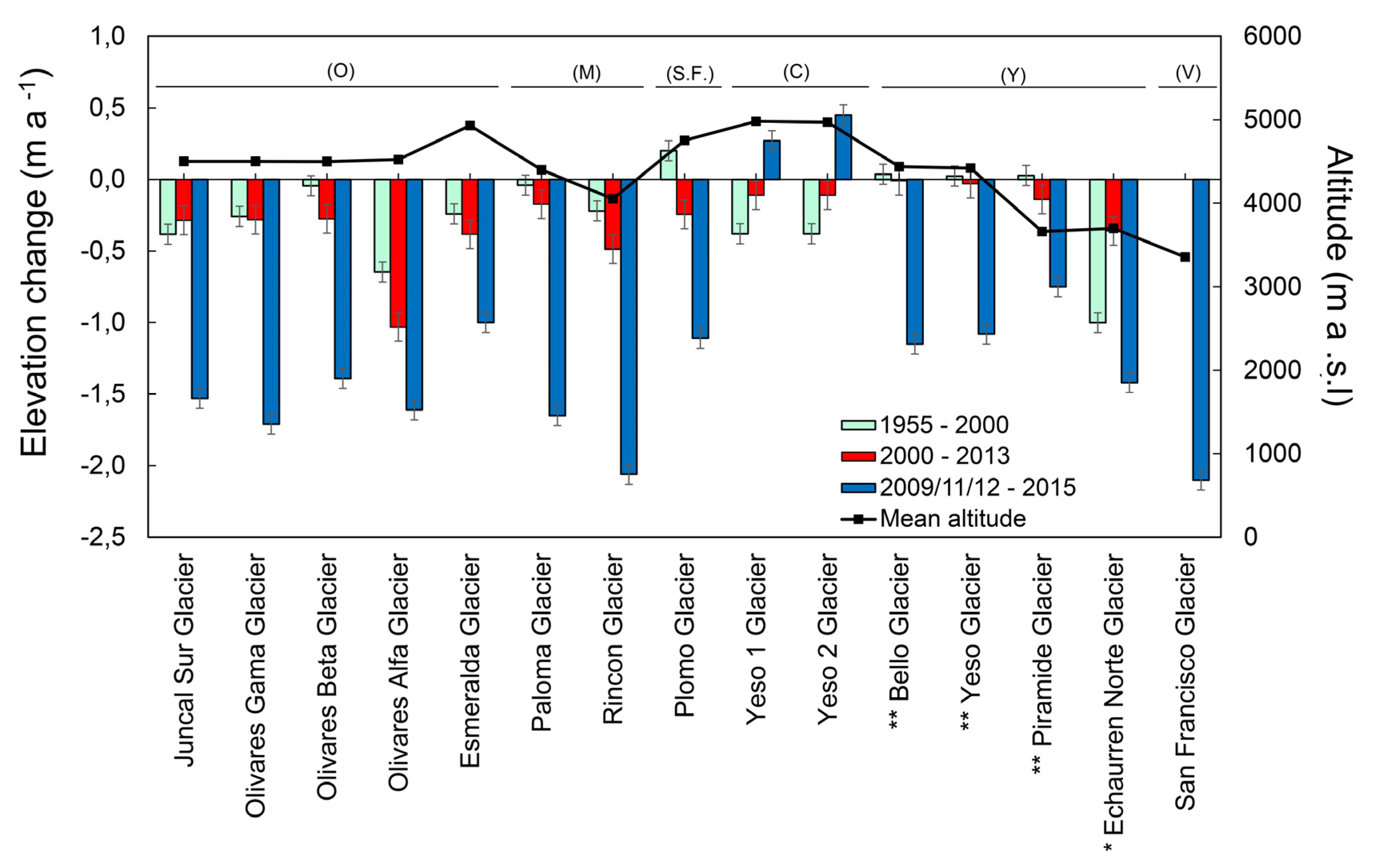
| Juncal Sur | Olivares | 20–29/04/2011 | 02–11/04/2015 | ~30 |
| Olivares Gama | Olivares | 20–29/04/2011 | 02–11/04/2015 | ~30 |
| Olivares Beta | Olivares | 20–29/04/2011 | 02–11/04/2015 | ~30 |
| Olivares Alfa | Olivares | 20–29/04/2011 | 02–11/04/2015 | ~30 |
| Esmeralda | Olivares | 30/04/2012 | 02–11/04/2015 | ~50 |
| Paloma | Molina | 30/04/2012 | 02–11/04/2015 | 100 |
| Rincón | Molina | 30/04/2012 | 02–11/04/2015 | 100 |
| Plomo | San Francisco | 30/04/2012 | 02–11/04/2015 | 100 |
| Yeso 1 | Colorado | 24/04/2012 | 23/02/2015 | 80 |
| Yeso 2 | Colorado | 24/04/2012 | 23/02/2015 | 100 |
| Bello | Yeso | 22/04/2012 | 26/02/2015 | 100 |
| Yeso | Yeso | 24/04/2012 | 17/02/2015 | 100 |
| Piramide | Yeso | 22/04/2012 | 23/03/2015 | 100 |
| Echaurren Norte | Yeso | 28/04/2009 | 23/02/2015 | 100 |
| San Francisco | Volcán | 29/04/2009 | 26/02/2015 | 100 |
| Sub-Basin | Area 2000 (km2) | Mass Balance Rate 1955–2000 (m w.e.a−1) | Mass Balance Rate 2000–2013 (m w.e.a−1) | Glacier Runoff Contribution |
|---|---|---|---|---|
| Olivares | 71.94 | −0.28 ± 0.07 | −0.32 ± 0.13 | Maipo River |
| Colorado | 63.11 | −0.18 ± 0.07 | 0.05 ± 0.12 | Maipo River |
| Yeso | 21.58 | −0.13 ± 0.07 | −0.15 ± 0.12 | Maipo River |
| Volcán | 50.22 | 0.14 ± 0.07 | −0.17 ± 0.13 | Maipo River |
| Maipo (Upper) | 46.56 | −0.01 ± 0.07 | −0.16 ± 0.13 | Maipo River |
| Rio Molina | 2.02 | 0.18 ± 0.07 | −0.17 ± 0.12 | Mapocho River |
| San Francisco | 3.01 | −0.04 ± 0.07 | −0.17 ± 0.13 | Mapocho River |
© 2020 by the authors. Licensee MDPI, Basel, Switzerland. This article is an open access article distributed under the terms and conditions of the Creative Commons Attribution (CC BY) license (http://creativecommons.org/licenses/by/4.0/).
Share and Cite
Farías-Barahona, D.; Ayala, Á.; Bravo, C.; Vivero, S.; Seehaus, T.; Vijay, S.; Schaefer, M.; Buglio, F.; Casassa, G.; Braun, M.H. 60 Years of Glacier Elevation and Mass Changes in the Maipo River Basin, Central Andes of Chile. Remote Sens. 2020, 12, 1658. https://doi.org/10.3390/rs12101658
Farías-Barahona D, Ayala Á, Bravo C, Vivero S, Seehaus T, Vijay S, Schaefer M, Buglio F, Casassa G, Braun MH. 60 Years of Glacier Elevation and Mass Changes in the Maipo River Basin, Central Andes of Chile. Remote Sensing. 2020; 12(10):1658. https://doi.org/10.3390/rs12101658
Chicago/Turabian StyleFarías-Barahona, David, Álvaro Ayala, Claudio Bravo, Sebastián Vivero, Thorsten Seehaus, Saurabh Vijay, Marius Schaefer, Franco Buglio, Gino Casassa, and Matthias H. Braun. 2020. "60 Years of Glacier Elevation and Mass Changes in the Maipo River Basin, Central Andes of Chile" Remote Sensing 12, no. 10: 1658. https://doi.org/10.3390/rs12101658