Global Calibration and Error Estimation of Altimeter, Scatterometer, and Radiometer Wind Speed Using Triple Collocation

Abstract

The accuracy of wind speed measurements is important in many applications. In the present work, error standard deviations of wind speed measured by satellites and National Data Buoy Center (NDBC) buoys were estimated using triple collocation. The satellites included six altimeters, three scatterometers, and four radiometers. The six altimeters were TOPEX, ERS-2, JASON-1, ENVISAT, JASON-2, and CRYOSAT-2, whilst the three scatterometers were QUIKSCAT, METOP-A, and METOP-B and the four radiometers included SSMI-F15, AMSR-2, WINDSAT, and GMI. Hence, a total of 14 platform measurements, including NDBC buoy data, were used and the error standard deviations of each estimated. It was found that altimeters have the smallest error standard deviations for wind speed measurements followed by scatterometers and then radiometers. NDBC buoys have the largest error standard deviation. Since triple collocation can simultaneously perform error estimation as well as calibration for a given reference, this method enables us to perform intercalibration between platform measurements including NDBC buoy. In addition, the calibration relations obtained from triple collocation were compared with the calibrations obtained from the widely used reduced major axis (RMA) regression approach. This method, to some extent, can accommodate measurements in which both platforms contain errors. The results showed that calibration relations obtained from RMA and triple collocation are very similar, as indicated by statistical parameters such as RMSE, correlation coefficient, scatter index, and bias.

1. Introduction

Global ocean wind speed data measured by a variety of different satellite platforms are now readily available in the public domain. These include altimeters, scatterometers, radiometers, and synthetic aperture radar (SAR). The durations of these satellite measurements amount to more than 30 years. The accuracy of these measurements is critical for a range of applications such as weather forecasting, the development of wind energy projects, model validations, monitoring of marine disasters, and wind climatology [1,2,3,4].

In order to improve the accuracy of the measurements, the satellite data have previously been calibrated and validated against in situ measurements by assuming that buoy measurements are the “ground truth” even though they are not free from errors [1]. However, although global wind data have been well calibrated and validated, they still contain measurement uncertainty and calibration inaccuracies. Hence, the estimation of these measurement errors is important.

Triple collocation is an approach which has been widely used to estimate the errors of a range of satellite measurements. This method was first introduced by Stoffelen [5] to estimate the wind vector component errors obtained from three different measurements, namely ERS-1 scatterometer, buoy data, and a forecast model. He found that NOAA buoys have the largest error variances whilst National Centers for Environmental Prediction (NCEP) model data have the smallest error variances on the spatial scale of the model. The method was used to calibrate measurements against a given reference data set, in this case moored buoys. The method has also been used to validate other satellite products such as soil moisture products [6,7,8,9,10,11], land water storage [12], precipitation products [13], atmospheric columnar integrated water vapor [14], and sea surface salinity [15]. In addition, the method has also been used to estimate wind speed errors of different satellite measurements [16,17,18,19]. Furthermore, the method has been extended by McColl et al. [20] by estimating the correlation coefficient of the measurement systems with respect to the unknown truth. This extension of triple collocation has been used to validate satellite surface albedo products [21].

Although triple collocation can be applied in a straightforward manner to estimate the error of measurements, the method has to satisfy the following assumptions, or the error estimation will be invalid. Since the method will involve three different measurements, the errors of each have to be uncorrelated. Moreover, linear calibration must be appropriate over the whole range of measurement values [22]. As shown in Young et al. [1] and Ribal and Young [23], high wind speeds of radiometers and QUIKSCAT scatterometer were calibrated nonlinearly. To address this issue in the application of triple collocation, we used the calibrated radiometers and QUIKSCAT scatterometer (i.e., linearized values).

Triple collocation can also be used to determine measurement calibration. Such an approach has been applied to OCEANSAT-2 calibration [18], ERS-1 scatterometer [5], ASCAT, and QUIKSCAT [24], and intercalibrations between satellites [19]. It should be noted that in order to calibrate a measurement using triple collocation, one of the three measurements has to be a reference. Hence, the other two measurements will be calibrated with respect to the reference. The reference can be in situ measurements or other satellites such as altimeters. The output of this calibration process will be the gradient or calibration factor (or scaling) and the offset or bias.

In relation to measurement calibration, there is another well-known method which has been extensively applied, so-called reduced major axis (RMA) regression [25]. This method is suitable for the calibration of measurements against reference data, where both measurement and reference contain errors. Such cases cannot be considered using conventional regression. RMA regression is also a powerful approach, as major outliers can be removed using robust regression [26]. Unlike conventional regression, which assumes that only one measurement contains errors, RMA, to some extent, can accommodate both measurements containing errors. RMA regression minimizes the triangular area bounded by the vertical and horizontal offsets between data points and the regression line and the cord of the regression line. This is different to conventional regression which only minimizes the vertical axis offsets from the regression line. Although both triple collocation and RMA regression have both been widely used for calibration purposes, we are not aware of a reference which compares the resulting calibration relations.

Therefore, the present work has two main goals. The first goal is to estimate the random error standard deviations of wind speed obtained from six altimeters, three scatterometers, and four radiometers as well as National Data Buoy Center (NDBC) buoy data. We also carry out intercalibrations between the various measurement platforms. The second goal of this work is to compare the calibration relationships obtained by applying the triple collocation method to the various satellite platforms with those obtained by using RMA regression. It should be noted that unlike other works, which usually involve data from numerical models, here, we only employ satellite data and NDBC buoy data.

Following this introduction, the source of each datasets that is used in this work is described in Section 2. The details of the triple collocation approach, including revisiting its derivation and its applications, will be presented in Section 3. This is followed by Section 4 in which the comparison calibrations between triple collocation and RMA regression are investigated. Discussion and conclusions are presented in Section 5 and Section 6, respectively.

2. Datasets

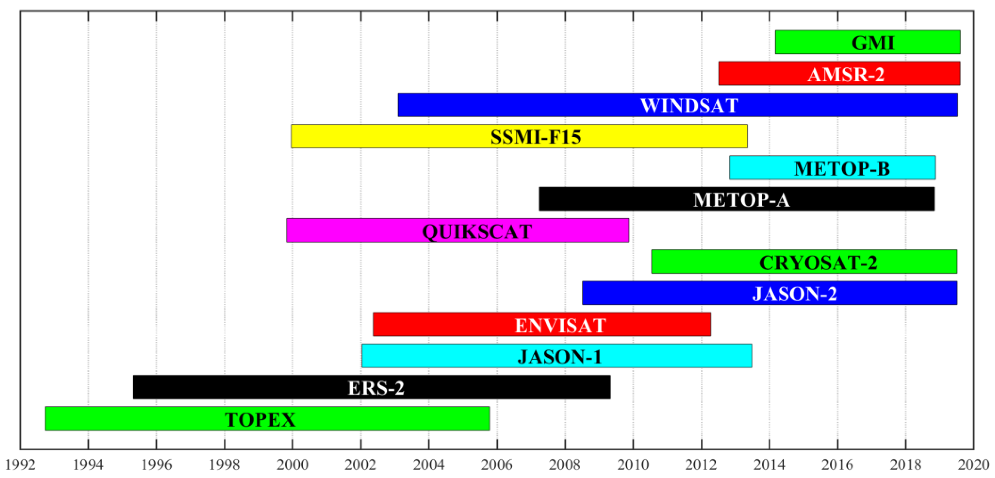
In order to conduct this study, data from a number of satellite missions are utilized. These missions includes six altimeters: TOPEX, ERS-2, JASON-1, ENVISAT, JASON-2, and CRYOSAT-2 (expressed in the order of launch), three scatterometers: QUIKSCAT, METOP-A, and METOP-B and four radiometers: SSMI-F15, AMSR-2, WINDSAT, and GMI. Hence a total of 13 satellites are used in this work. Figure 1 shows the periods in which all instruments were active. Details of each satellite are provided in the following sub-sections, including their respective data sources.

2.1. Altimeter Data

Since 1985, there have been 14 altimeters that have been launched for ocean wind speed and significant wave height observations. Altimeters measure the radar cross-section, $\sigma$, which is the ratio of the transmitted to received radar energy along a nadir track below the satellite [27]. This radar cross-section can be related to wind speed using a non-linear function. As the altimeter measures only over a narrow footprint (approximately 10 km) directly below the satellite, the resolution of altimeter data along the track is high (measurement every approximately 10 km) but the cross-track separation is large (of order 500 km) [1]. However, it has been shown by comparison with in situ data that altimeter measurements are in good agreement with buoy and platform measurements, including at high wind speeds (>18 m/s) [23].

An extensive data set of calibrated altimeter data has been archived on the Australian Ocean Data Network (AODN), by Ribal and Young [4]. This archive includes a total of 14 altimeters, namely GEOSAT, ERS-1, TOPEX, ERS-2, GFO, JASON-1, ENVISAT, JASON-2, CRYOSAT-2, HY-2A, SARAL, JASON-3, SENTINEL-3A, and SENTINEL-3B (expressed in the order of launch). The database is updated every six months and presently includes data from 1985 to 31 December 2019. The Ribal and Young [4] database determines the wind speed, $U_{10}$ by firstly extracting the 1Hz radar cross-section, ${\sigma }_0$ for each altimeter. The Abdalla [28] relationship between $U_{10}$ and ${\sigma }_0$ is then used to obtain a first approximation to the wind speed. A further linear least-squares correction based on buoy match-up data is then applied to produce the 1Hz calibrated altimeter wind speed product.

For the present work, six of these altimeter missions were used, namely TOPEX, ERS-2, JASON-1, ENVISAT, JASON-2, and CRYOSAT-2 for error estimation and intercalibration based on triple collocation. This subset of altimeter missions was used as they are of long duration and overlap in time with the other satellite platform to be used.

2.2. Scatterometer Data

Unlike altimeters, which measure the radar cross-section at nadir along the track, scatterometers measure radar cross-section over a broad swath. Hence, cross-track resolution is increased significantly (25 km with a swath up to 1400 km wide) compared to the altimeters, but along-track resolution is slightly decreased (typically 25 km). The swath configuration of the scatterometers depend on their antenna configuration [23].

The first scatterometer mission to provide global data was ERS-1, which was launched in 1991. Following ERA-1 a series of scatterometers have provided continuous global coverage to the present day. Recently, Ribal and Young [23] have calibrated and cross-validated seven different scatterometers and archived calibrated and quality controlled data for the period 1992–2018 on the AODN (see the details including the procedure to obtain the data in Ribal and Young [23]). The Ribal and Young [23] scatterometer database takes wind speed data from the respective satellite mission repositories for each scatterometer and then applies a linear least-squares correction based on buoy match-up data to obtain the final wind speed product. The seven scatterometers in the database are ERS-1, ERS-2, QUIKSCAT, METOP-A, OCEANSAT-2, METOP-B, and RAPIDSCAT (also expressed in the order of launch). The database is also updated every six months and presently includes data from 1992 to 2 April 2020. It should be noted that most of the scatterometers are in sun-synchronous orbits except RAPIDSCAT. These orbit details are important when considering collocations with other satellites platforms.

The total duration of the available scatterometer dataset is approximately 27 years. In the present work, the QUIKSCAT, METOP-A and METOP-B scatterometer missions have been used. This sub-set was used as the time period overlaps with the other satellite platforms used and the satellite orbits are such that collocations occur with the other missions. The grid resolution of QUIKSCAT is 12.5 km while the grid resolution of METOP-A and METOP-B is 25 km.

2.3. Radiometer Data

Similar to scatterometer, radiometer also measures over a swath which is approximately 1400 km wide with a grid resolution of 25 km [1,29]. Moreover, radiometers are also generally placed in sun-synchronous orbits. While scatterometers measure radar cross-section, radiometers measure brightness temperature of the sea surface. This measurement is related to the emissivity and reflectivity of the ocean surface at the frequency of the radiometer. These properties are in turn related to the roughness of the water surface and hence the wind stress. The wind stress is then related to the wind speed assuming a neutrally stable atmospheric boundary layer and a constant value of drag coefficient [29,30,31,32]. Radiometers are particularly impacted by heavy rain, making the recovery of reliable wind speed measurements problematic in such situations [33]. Although both altimeter and scatterometer data does degrade in heavy rain events, these instruments are far less impacted than radiometers, notably ERS and ASCAT which operate at C-band.

A calibrated and cross-validated dataset of radiometers from 1991 is described in Young et al. [1]. In relation to the present work, four radiometer missions from this combined dataset were used: SSMI-F15, AMSR-2, WINDSAT, and GMI. The durations of these selected radiometers are presented in Figure 1. The raw data for these radiometers were obtained from Remote Sensing Systems (REMSS) (http://www.remss.com/) [1]. Consistent with the altimeter and scatterometer processing, the wind speed values obtained from REMSS were calibrated using a linear least-squares correction based on buoy match-up data [1].

2.4. National Data Buoy Center (NDBC) Buoy Data

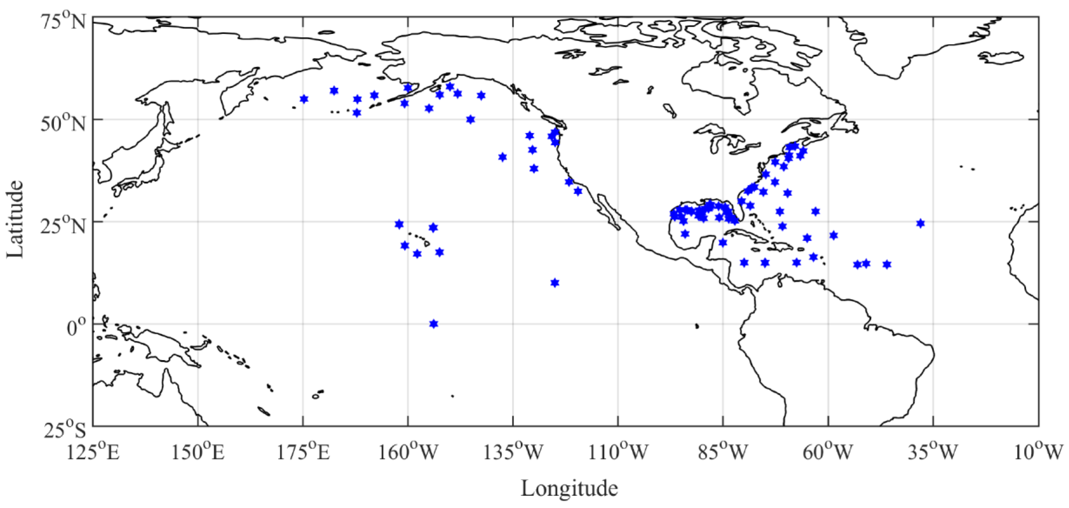
In addition to considering error estimation of the satellite data described above, errors for wind speed data obtained from National Data Buoy Center (NDBC) anemometer data has also been considered in this study. Although buoy data is usually assumed as the “ground truth”, random errors and accuracy of such data must also be considered. The NDBC buoy data used in this work were obtained from the National Oceanographic Data Center (NODC, https://data.nodc.noaa.gov/thredds/catalog/ndbc/cmanwx/catalog.html), and are publicly available under NOAA’s National Centers for Environment Information (NCEI). In order to ensure collocated satellite data are not impacted by the proximity of land, only buoys which are more than 50 km from a coastline were used. NDBC data include quality flags of 0, 1, 2, and 3, representing quality_good, out_of_range, sensor_nonfunctional, and questionable, respectively. In order to ensure high quality data, only wind speeds flagged “0” were used. NDBC data before 2011 do not have quality flags, however, as reported in Ribal and Young [23], the data indicate few clear outliers. The locations of the buoys used are presented in Figure 2.

Buoys measure wind speed at the height of anemometer z $\left(U_z\right),$ where each buoy has a different anemometer height. All data were converted to a consistent reference height of 10 m assuming a neutral stability boundary layer and a logarithmic profile (e.g., [34,35]):

$$U_{10}=U_z\sqrt{\frac{{\kappa }^2}{C_d}}\frac{1}{\ln \left(z/z_0\right)},$$

(1)

where $\kappa$ is the von Kármán constant which is approximately 0.4, $C_d$ and $z_0$ are the drag coefficient and the roughness length, respectively. In the present work, values of $C_d$ and $z_0$ were assumed as $1.2\times {10}^{-3}$ and $9.7\times {10}^{-5} \mathrm{m}$, respectively. These values have previously been adopted by Young et al. [1] and Ribal and Young [4,23]. As noted by Young et al. [1], a different assumption for the value of $C_d$ does not have a major impact on the final satellite wind speed [36].

3. Triple Collocation Method

3.1. Derivation of the Calibration Scheme

As previously noted, triple collocation has been widely used to estimate the accuracy of measurements either from satellites or buoy data. In most previous derivations of triple collocation, it has been assumed that one or all of the measurement systems have uncorrelated errors, or the correlation is specified. However, in the present derivation, we will remove this constraint and allow errors of the three systems to be correlated.

It is assumed that there are three different measurement systems, $X_i, i=1,2,3$, in which all measurements are related to the true value T through the following linear relation [16,20,24]:

$$X_i=a_i+b_{i}T+e_i$$

(2)

where $a_i$ and $b_i$ (i = 1, 2, 3) are the offset and the slope of the calibration, respectively and $e_i$ is the random measurement error in system i. It is assumed that the random measurement error is free from bias and hence, $\langle e_i\rangle =0$. Moreover, the variance of random measurement errors, $\langle e_i^2\rangle$, is assumed not to be dependent on T over the whole period of wind speed measurements.

$X_1$ is assumed to be the reference, which could be buoys or altimeters or any of the other measurement system. Hence, the other two systems, namely $X_2$ and $X_3$ are calibrated with respect to the reference. As a result, Equation (2) becomes:

$$\begin{gathered} X_1=T+e_1 \\ {X}_2=a_2+b_{2}T+e_2 \\ {X}_3=a_3+b_{3}T+e_3 \end{gathered}$$

(3)

Following a similar procedure to Vogelzang and Stoffelen [22] but without specifying the correlation of the errors of the systems, the slopes of the calibrations of the two systems are given by:

$$b_2=\frac{C_{23}-\langle e_2{e}_3\rangle }{C_{13}-\langle e_1{e}_3\rangle }$$

(4)

and

$$b_3=\frac{C_{23}-\langle e_2{e}_3\rangle }{C_{12}-\langle e_1{e}_2\rangle }$$

(5)

where $\langle e_i{e}_j\rangle$ is the error covariance between system i and system j, $C_{ij}$ is the covariance between system i and j, $C_{ij}=cov\left(X_i,X_j\right)$, $C_{ii}=var\left(X_i\right)$, determined from the N data values as $cov\left(X_i,X_j\right)=\frac{1}{N}{\sum }_{k=1}^N{X}_{ik}{X}_{jk}-{\overline{X}}_i{\overline{X}}_j$. The covariance, $C_{ij}$ can be related to the first and the second (mixed) order moments, $M_i$ and $M_{ij}$ of datasets i and j, where $M_i={\overline{X}}_i=\langle X_i\rangle =\frac{1}{N}{\sum }_{k=1}^N{X}_{ik}$, by the relationship

$$C_{ij}=M_{ij}-M_i{M}_j$$

(6)

Equation (4) is the same as Equation (13) of Abdalla and Chiara [19] and also Equation (13) of Su et al. [11], if the error covariances are zero which means that the random errors in the systems are uncorrelated.

Similarly, the offsets of the calibration relationships of two systems are given by

$$a_2=M_2-b_2{M}_1 \mathrm{and} a_3=M_3-b_3{M}_1$$

(7)

The error variances can be written as:

$$\begin{gathered} {\sigma }_1^2=C_{11}-\frac{\left(C_{12}-\langle e_1{e}_2\rangle \right)\left(C_{13}-\langle e_1{e}_3\rangle \right)}{C_{23}-\langle e_2{e}_3\rangle } \\ {\sigma }_2^2=C_{22}-\frac{\left(C_{12}-\langle e_1{e}_2\rangle \right)\left(C_{23}-\langle e_2{e}_3\rangle \right)}{C_{13}-\langle e_1{e}_3\rangle } \\ {\sigma }_3^2=C_{33}-\frac{\left(C_{23}-\langle e_2{e}_3\rangle \right)\left(C_{13}-\langle e_1{e}_3\rangle \right)}{C_{12}-\langle e_1{e}_2\rangle } \end{gathered}$$

(8)

Equations (8) contain six unknowns, namely three error covariances on the right-hand side of the equations and three error variances on the left-hand side, with only three equations. In order to make the problem tractable, additional assumptions are required. The simplest assumption is to assume that the error covariances of all measurement systems are zero. This assumption will remove three unknowns and yields a system of three equations in three unknowns. However, this assumption does not always hold, an illustration of such a case can be found in Stoffelen [5], Vogelzang et al. [24] and Abdalla and Chiara [19]. It should be noted that Equation (8) reduces to Equation (4) of Nearing et al. [37] when it is assumed that all errors from the measuring systems are uncorrelated, e.g., $\langle e_i{e}_j\rangle =0, \mathrm{where} i,j=1,2,3 \mathrm{and} i\ne j.$ Error standard deviations are obtained by taking the square root of error variances.

3.2. Control Conditions for Data Collocation

In order to estimate the error of any measurements using triple collocation, one has to find matchups of three different measurement systems, with given collocation conditions (CC). When NDBC buoys are included in the triple collocation, then, as mentioned above, only buoys which have a reported anemometer height and are more than 50 km from the coastline are used. In order to find matchups of three measurements, both spatial and temporal separation criteria were adopted [19]. A one-degree spatial separation criteria, for which only measurements less than approximately 100 km (1 degree) from the selected buoy were considered. Similarly, a 60-min temporal separation criterion, where only measurements which occurred within 60-min of the buoy recording data, was used. In addition, a minimum of five wind vector cells were required within a 100 km radius region around the buoy. Finally, large variability in the satellite data wind speed were excluded, by rejecting matchup data for which $\sigma \left(U_{10}\right)/{\overline{U}}_{10}>0.2$, where $\sigma \left(U_{10}\right)$ and ${\overline{U}}_{10}$ are the standard deviation and mean, respectively, of wind speed measurements within a radius of 100 km from the buoy. Similar criteria have been applied for the matchups between satellites. It should be noted that all altimeter, radiometer, and scatterometer data used in this analysis have had a land mask applied to ensure there are no matchups potentially contaminated by land.

3.3. Wind Speed Errors

Error standard deviations of the six altimeters, three scatterometers, and four radiometers shown in Figure 1 were determined using triple collocation. In addition, as indicated above, the random error standard deviation of NDBC buoy will also be estimated. Since the selected satellites do not operate at the same time, the combinations of the three platforms cannot be selected randomly. The possible combinations of the measurement platforms which meet the matchup criteria are shown in

Table 1. All possible triplet-collocated datasets and their random error standard deviations shown in the parentheses. N is the number of matchups after quality assurance criteria are applied, O is the number of outliers, and C=N-O is the number of observations used to estimate the error variances.

No.	Altimeters/NDBC (Error Standard Deviation (m/s))	Scatterometers (Error Standard Deviation (m/s))	Radiometers (Error Standard Deviation (m/s))	N	O	C
1.	TOPEX (0.524)	QUIKSCAT (0.391)	F15 (0.794)	35,795	228	35,567
2.	ERS-2 (0.605)	QUIKSCAT (0.473)	F15 (0.673)	15,143	77	15,066
3.	JASON-1 (0.571)	QUIKSCAT (0.387)	F15 (0.771)	94,779	825	93,954
4.	ENVISAT (0.545)	QUIKSCAT (0.463)	F15 (0.637)	27,136	305	26,831
5.	JASON-2 (0.538)	METOP-A (0.546)	AMSR-2 (0.682)	23,677	218	23,459
6.	JASON-2 (0.284)	METOP-A (1.022)	WINDSAT (0.723)	34,424	219	34,205
7.	JASON-2 (0.574)	METOP-A (0.643)	GMI (0.602)	27,297	306	26,991
8.	JASON-2 (0.547)	METOP-B (0.547)	AMSR-2 (0.667)	23,592	210	23,382
9.	JASON-2 (0.257)	METOP-B (1.011)	WINDSAT (0.725)	21,100	157	20,943
10.	JASON-2 (0.578)	METOP-B (0.635)	GMI (0.607)	26,889	318	26,571
11.	CRYOSAT-2 (0.505)	METOP-A (0.555)	AMSR-2 (0.710)	13,487	172	13,315
12.	CRYOSAT-2 (0.310)	METOP-A (0.899)	WINDSAT (0.670)	19,745	180	19,565
13.	NDBC (0.833)	METOP-A (0.542)	WINDSAT (0.725)	58,313	814	57,499
14	NDBC (0.840)	METOP-B (0.523)	WINDSAT (0.698)	39,389	636	38,753

.

In order to estimate the error variances, it is assumed that the random errors in the three different measurements are uncorrelated. For the present datasets, this is believed to be a reasonable assumption, as each system senses the wind using independent processes (i.e., nadir radar cross-section—altimeter; off-nadir multiple-look radar cross-section—scatterometer; brightness temperature—radiometer; anemometer—buoys). The assumption of uncorrelated errors is more questionable, when model reanalysis data is used in which satellite wind speeds have been assimilated into the model. Hence, all error covariances are assumed approximately zero and Equation (8) can be simplified to:

$$\begin{gathered} {\sigma }_1^2=C_{11}-\frac{C_{12}{C}_{13}}{C_{23}} \\ {\sigma }_2^2=C_{22}-\frac{C_{12}{C}_{23}}{C_{13}} \\ {\sigma }_3^2=C_{33}-\frac{C_{23}{C}_{13}}{C_{12}} \end{gathered}$$

(9)

Figure 3a,b show examples of the wind speed error standard deviations, ${\sigma }_i$, calculated based on yearly data for two sets of collocation triplets [TOPEX (alt.), QUIKSCAT (scat.), SSMI-F15 (rad.)] and [JASON-1 (alt.), QUIKSCAT (scat.), SSMI-F15 (rad.)]. It is clear that the error standard deviations, ${\sigma }_i$, are almost constant over the observation period, indication no significant changes in the errors, ${\sigma }_i$, as a function of time, as expected. Moreover, Figure 3c,d show the corresponding number of observations used to estimate the random errors per year in Figure 3a,b It is important to note that it is not recommended to calculate the error variances based on monthly data, as the number of observations will be relatively small over such periods, leading to unrepresentative statistics [19]. It should be noted that these annual statistics are calculated from all triplet matchups and hence implicitly account for seasonal variations in wind speed and zonal variations across the globe.

Applying Equation (9), the error standard deviations (${\sigma }_i$) for all cases are summarized in Table 1 (in parentheses). Note that, as previously mentioned, error standard deviations are defined as the square root of error variances. The number of matchups is typically a few hundred thousand but after applying the quality control conditions (see data collocation section), the quality data is typically reduced to approximately 20% of this figure. Stoffelen [5] has proposed a condition for quality control of triple collocation where some collocation triplets can be rejected as they are clear outliers. In the present work, we used robust regression with reduced major axis regression to exclude the outliers from the triplets [4]. Testing indicated this produced results very similar to the method of Stoffelen [5]. The number of excluded outliers for each triplet are presented in Table 1 (column labelled “O”). All outliers are excluded in determining the error variances. The resulting number of “clean” data collocation values used for error estimations as summarized in Table 1 (column labelled “C”).

Where a platform is present in multiple triplets in Table 1, the mean error standard deviation is computed for each platform by averaging the error standard deviation for each triplet. The average result is then reported in

Table 2. Average random error standard deviations for measurement systems.

No.	Satellite Measurements	Mean Error Standard Deviation (m/s)	Mean Error Standard Deviation for Platform Type (m/s)
1.	TOPEX	0.524	0.519
2.	ERS-2	0.605
3.	JASON-1	0.571
4.	ENVISAT	0.545
5.	JASON-2	0.463
6.	CRYOSAT-2	0.407
7.	QUIKSCAT	0.428	0.603
8.	METOP-A	0.701
9.	METOP-B	0.679
10.	SSMI-F15	0.719	0.679
11.	AMSR-2	0.686
12.	WINDSAT	0.708
13.	GMI	0.604
14.	NDBC	0.837	0.837

. This table includes the average error standard deviation for both satellite systems and NDBC buoys. The four platform groups, namely altimeters, scatterometers, radiometers, and NDBC buoys are found to have average error standard deviations of 0.519 m/s, 0.603 m/s, 0.679 m/s, and 0.837 m/s, for altimeter, scatterometer, radiometer, and NDBC buoy, respectively. This indicates that altimeters have the smallest random errors for wind speed measurements, followed by scatterometers and then radiometers. It should be noted that, although altimeters generally show smaller error standard deviation than scatterometers, as is revealed in Table 1, the QUIKSCAT scatterometer has high quality measurements.

The results also show that NDBC buoys have the largest error standard deviations. This result is similar to what has been reported by Stoffelen [5] where NDBC buoys had larger error variances than ERS scatterometer and the NCEP forecast model. Stoffelen argued that the main reason for NDBC buoys having relatively large error variances is due to the spatial representativeness error: the buoys measure small-scale signals that are not detected by the other systems. That is, the NDBC buoy data are point measurements averaged over a short period of time, whereas the satellite and model products are averages over the relatively large satellite footprint or model grid square.

As noted above, Figure 3 shows two selected cases for the error standard deviation wind speeds calculated on a yearly basis. Both cases use altimeters as the reference. As can be seen from the figures, the average random errors are almost the same as obtained when using all the data and reported in Table 1 and Table 2. For completeness, it should be noted that the triplet-collocations between TOPEX, QUIKSCAT and SSMI-F15 have some matchups in 1999 but there are a total of only 16 matchups which passed the quality assurance process, hence the yearly estimated error standard deviation for 1999 has been excluded. However, these matchups have been included when estimating the total error variances.

3.4. Calibrations Based on Triple Collocation

Starting from Equation (3), it is assumed that $X_1$ is the reference, which in this case would be an altimeter or in situ buoys. Hence, the calibration relations for scatterometers and radiometers against the reference can be written as

$$X_2^{*}=\frac{X_2}{b_2}-\frac{a_2}{b_2}$$

(10)

and

$$X_3^{*}=\frac{X_3}{b_3}-\frac{a_3}{b_3},$$

(11)

respectively, where $a_2,a_3, b_2$ and $b_3$ are given in Equations (4), (5) and (7). $X_i$ and $X_i^{*}$ are uncalibrated and calibrated data, respectively.

Similarly, intercalibration relations between scatterometers and radiometers are given by

$$X_3^{*}=a_4+b_4{X}_3\hspace{1em}\left(if X_2 is the reference\right)$$

(12)

or

$$X_2^{*}=\frac{X_2}{b_4}-\frac{a_4}{b_4}\hspace{1em}\left(if X_3 is the reference\right)$$

(13)

where $a_4=a_2-\frac{a_3{b}_2}{b_3} \mathrm{and} b_4=\frac{b_2}{b_3}.$

By using the measurements from the altimeter as reference, the offset, a_i, and slope, b_i, coefficients in Equations (10) and (11) were calibrated. Values from the calibrating operation are reported in

Table 3. Calibration coefficient slopes $\left(b_i\right)$ and offsets $\left(a_i\right)$ for the triplet collocated altimeter $(X_1)$, scatterometer $\left(X_2\right)$ and radiometer $\left(X_3\right)$ wind speed. Empty cells mean no collocation has been performed and altimeter is the reference. All other parameters as noted above.

Altimeters	Scatterometers				Radiometers
		QS	MA	MB		F15	AM	WS	GMI
TP	$a_2$	−0.2964			$a_3$	−0.0062
	$b_2$	0.9918			$b_3$	0.9448
E2	$a_2$	−0.0847			$a_3$	−0.0794
	$b_2$	0.9785			$b_3$	0.9722
J1	$a_2$	−0.0911			$a_3$	0.1769
	$b_2$	0.9787			$b_3$	0.9394
EV	$a_2$	−0.2669			$a_3$	−0.0729
	$b_2$	0.9706			$b_3$	0.9455
J2	$a_2$		0.1408		$a_3$		−0.1341
	$b_2$		0.9270		$b_3$		0.9442
	$a_2$		0.2169		$a_3$				0.1607
	$b_2$		0.9180		$b_3$				0.9235
	$a_2$		0.5471		$a_3$			0.3564
	$b_2$		0.8909		$b_3$			0.9137
	$a_2$			0.1276	$a_3$		−0.1429
	$b_2$			0.9331	$b_3$		0.9445
	$a_2$			0.4693				0.2270
	$b_2$			0.8977				0.9183
	$a_2$			0.2287					0.1409
	$b_2$			0.9225					0.9257
C2	$a_2$		0.5259				0.4919
	$b_2$		0.9214				0.9167
	$a_2$		0.6916					0.8028
	$b_2$		0.9036					0.8898

for all the platforms investigated. Likewise, using Equation (13) and choosing the radiometer as reference, the scatterometer can be calibrated. In this case the values of offset, a₄, and slope, b₄, are summarized in

Table 4. Calibration coefficients slope $\left(b_4\right)$ and offsets $\left(a_4\right)$ for intercalibrations between scatterometers $\left(X_2\right)$ and radiometers $\left(X_3\right)$ wind speed in which radiometer is the reference. Empty cells mean no calibration has been performed. All other parameters as noted above.

Radiometers		Scatterometers			Altimeters Used in Triplet
		QUIKSCAT	METOP-A	METOP-B
SSMI-F15	$a_4$	−0.2899			TOPEX
	$b_4$	1.0498
	$a_4$	−0.0047			ERS-2
	$b_4$	1.0065
	$a_4$	−0.2755			JASON-1
	$b_4$	1.0418
	$a_4$.	−0.1921			ENVISAT
	$b_4$	1.0265
AMSR-2	$a_4$		0.2725	0.2688	JASON-2
	$b_4$		0.9818	0.9879
	$a_4$.		0.0315		CRYOSAT-2
	$b_4$		1.0052
WINDSAT	$a_4$		0.1996	0.2474	JASON-2
	$b_4$.		0.9750	0.9775
	$a_4$		−0.1237		CRYOSAT-2
	$b_4$		1.0156
GMI	$a_4$		0.0571	0.0883	JASON-2
	$b_4$		0.9940	0.9966

, along with the altimeter used (right column Table 4), for all the platforms investigated. Note that TP, E2, J1, EV, J2, and C2 in the table are abbreviated forms of altimeters TOPEX, ERS-2, JASON-1, ENVISAT, JASON-2, and CRYOSAT-2, respectively. Likewise, for scatterometers and radiometers, QS, MA, MB, F15, AM, and WS are abbreviated forms of QUIKSCAT, METOP-A, METOP-B, SSMI-F15, AMSR-2, and WINDSAT, respectively. Moreover, index i has values of 2 and 3 which represent scatterometer and radiometer. As mentioned earlier, the altimeters are taken as the reference.

4. Comparison Calibrations between Reduced Major Axis (RMA) and Triple Collocations

In order to compare the calibration relations obtained from triple collocation and reduced major axis regression, two different cases were considered. Firstly, NDBC buoy data were considered as the reference and then scatterometer and radiometer were calibrated with respect to the reference. Secondly, intercalibrations between scatterometer and radiometer were performed. For the latter case, radiometer was considered as the reference.

As previously applied [1,4,23,36], reduced major axis (RMA) regression can accommodate two different measurements, both of which contain random errors [25]. This regression approach minimizes the triangular region, bounded by the vertical and horizontal lines between data points and the regression line, and the cord of the regression line. This differs from traditional regression which assumes that one of the measurements does not contain any errors and hence only minimizes the vertical offsets from regression line. Moreover, standard least squares regression analysis is very sensitive to outliers, which can be removed using robust regression [26]. Robust regression removes outliers using iteratively reweighted least-squares [26]. In this method, for each point, robust regression assigns a weight with values between 0 and 1. The weights for all points are obtained and then all values with weights which were less than 0.01 were defined as outliers and removed from subsequent analysis before applying the RMA regression analysis.

In order to compare the resulting calibration relations between RMA and triple collocation, four different statistical parameters were evaluated. These statistical parameters are bias (B), root-mean square error (RMSE), Pierson’s correlation coefficient ($\rho$), and scatter index (SI). These parameters were calculated using the following equations in which M and O stand for model and observation, respectively, and N is the number of data used [4,23,38].

$$B=\frac{1}{N}{\displaystyle \sum }_{i=1}^N\left(M_i-O_i\right)$$

(14)

$$RMSE=\sqrt{\frac{1}{N}{\displaystyle \sum }_{i=1}^N{\left(M_i-O_i\right)}^2}$$

(15)

$$SI=\frac{\sqrt{\frac{1}{N}{\sum }_{i=1}^N{\left(M_i-O_i-B\right)}^2}}{\frac{1}{N}{\sum }_{i=1}^N{O}_i}$$

(16)

$$\rho =\frac{cov(M,O)}{\sqrt{cov(M)cov(O)}}$$

(17)

Two triplet combinations were considered as examples: (a) METOP-A (scatterometer), WINDSAT (radiometer) and NDBC and (b): METOP-B (scatterometer), WINDSAT (radiometer) and NDBC. The calibration of the scatterometers and a radiometer with respect to NDBC buoy data are given by Equations (10) and (11). Similarly, the calibration relations of the scatterometers with respect to the radiometer are obtained from Equation (13). For simplicity, the figures below do not show the results involving METOP-B.

Figure 4 shows the comparisons between calibration relations obtained from RMA regression and triple collocation between METOP-A and NDBC data. As can be seen from the figure, the calibration relations differ slightly in terms of slope and offset. However, the statistical parameters [Equations (14)–(17)], are very similar, with the correlation coefficient agreeing to four decimal places. The RMSE values differ by only 1.19 cm/s and the scatter index values differ by only 0.14%. It should be noted that the RMA regression calibration relation between METOP-A and NDBC buoy data is almost the same as that previously found by Ribal and Young [23], the small differences due to slightly different collocation datasets. Similar good agreement between the two approaches were also found for METOP-B (figure is not shown). The detailed calibration relations are shown in

Table 5. Comparison of calibration relations obtained from RMA regression and triple collocation (TC). MA, MB, and WS are abbreviated forms of METOP-A, METOP-B, and WINDSAT, respectively. $U_{10}^{*}$ is the calibrated value and $U_{10}$ is the uncalibrated data. Also shown are the confidence limits on the RMA regression, number of points, N, and the percentage of outliers from the robust regression.

Scat	Method	Calibration Relation	95% Limit Slope	95% Limit Offset	N	% Outliers	Ref.
MA	RMA	$U_{10}^{*}=1.040U_{10}-0.199$	1.037 to 1.043	−0.225 to −0.173	57,499	0.91	NDBC
	TC	$U_{10}^{*}=1.010U_{10}+0.050$
WS	RMA	$U_{10}^{*}=1.061U_{10}-0.513$	1.058 to 1.065	−0.543 to −0.483		0.84
	TC	$U_{10}^{*}=1.052U_{10}-0.431$
MA	RMA	$U_{10}^{*}=0.979U_{10}+0.306$	0.976 to 0.982	0.283 to 0.328		0.34	WS
	TC	$U_{10}^{*}=0.960U_{10}+0.458$
MB	RMA	$U_{10}^{*}=1.028U_{10}-0.129$	1.024 to 1.032	−0.161 to −0.096	38,753	1.10	NDBC
	TC	$U_{10}^{*}=0.990U_{10}+0.182$
WS	RMA	$U_{10}^{*}=1.055U_{10}-0.479$	1.051 to 1.060	−0.517 to −0.442		1.06
	TC	$U_{10}^{*}=1.039U_{10}-0.344$
MB	RMA	$U_{10}^{*}=0.972U_{10}+0.353$	0.969 to 0.975	0.326 to 0.381		0.35	WS
	TC	$U_{10}^{*}=0.953U_{10}+0.507$

. In Figure 4 (and subsequently in Figure 5 and Figure 6) the outliers randomly scatter outside two lines which run parallel to the RMA regression line. The reason for this structure is that we chose an arbitrary value of 0.01 for the robust regression weight to define the outliers. The lines parallel to the RMA regression result represent this limit.

Similarly to Figure 4, Figure 5 shows the comparison of the calibration relations obtained from RMA regression and triple collocation approaches between WINDSAT and NDBC buoy data. Again, the agreement between the approaches is excellent, with the correlation coefficients being the same to four decimal places, an RMSE difference of 0.47 cm/s and the scatter index difference of only 0.06%. In addition, the calibration relations obtained from triplet-collocated NDBC buoy, METOP-B and WINDSAT are almost the same as obtained from triplet-collocated NDBC buoy, METOP-A and WINDSAT as shown in Table 5. This follows the findings of Ribal and Young [23] that the calibration relationships for METOP-A and METOP-B are almost identical.

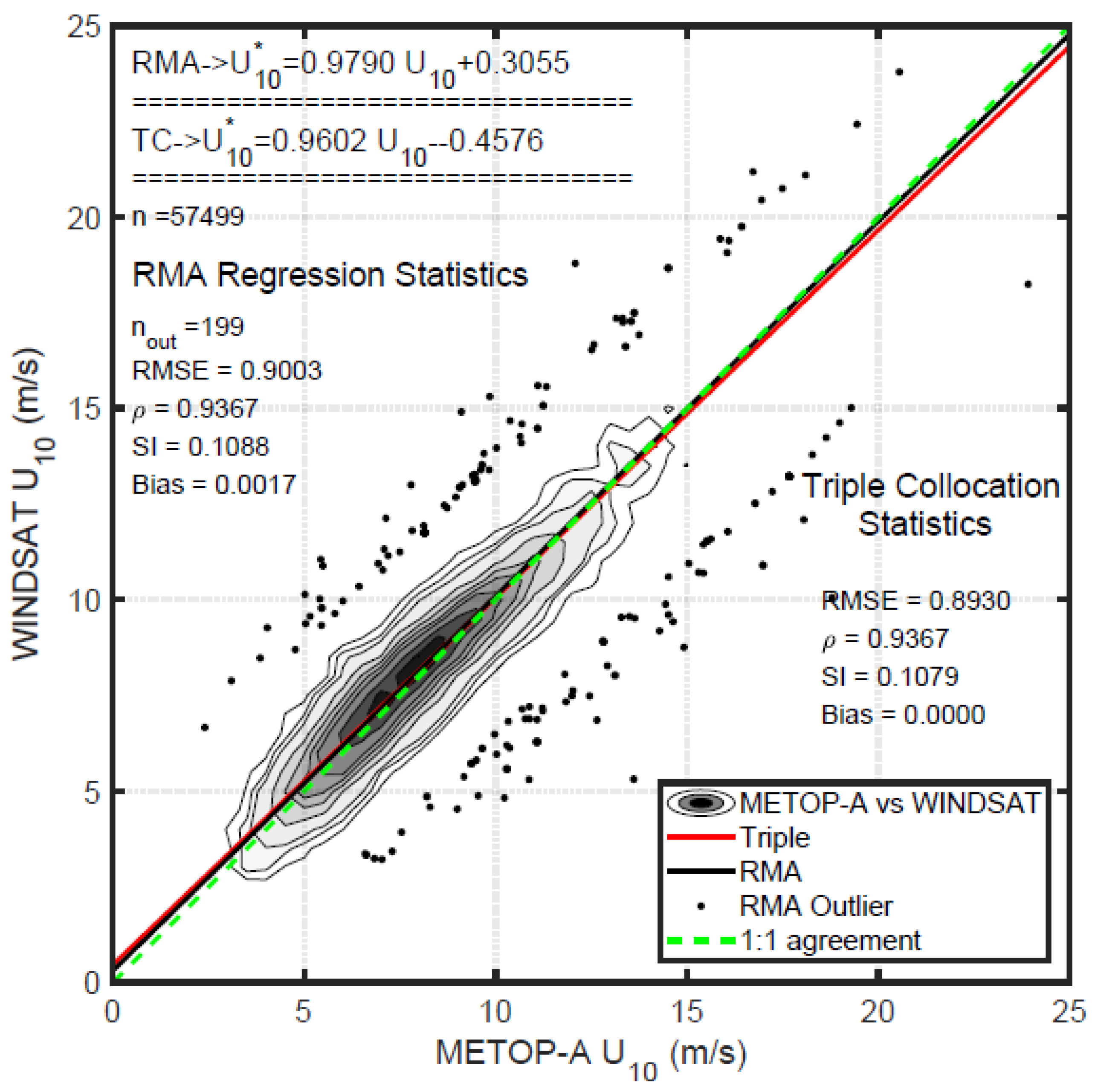
As noted above, this approach can also calibrate the scatterometers METOP-A and METOP-B with respect to the radiometer WINDSAT. As shown in Figure 6 (METOP-A with respect to WINDSAT), the calibration relations obtained from RMA regression and triple collocation are again very similar, with the offsets having the same sign. In terms of statistical parameters, the correlation coefficient is the same to 4 decimal places and RMSE and scatter index differ by 0.73 cm/s and 0.09%, respectively. A similar result was obtained when METOP-B was calibrated with respect to WINDSAT, with the details provided in Table 5.

Examination of Table 5 shows that triple collocation and RMA regression produce very similar calibration relations across all the satellites. Therefore, in order to calibrate a measurement system with respect to another system, it appears sufficient to only employ RMA regression, unless one is interested in error estimation of the systems. Calibrating a measurement system with respect to another system using RMA regression requires only two systems which can lead to a higher number of matchups, whereas the requirements of three independent measurements with triple collocation typically results in a much smaller collocation dataset. Finally, triple collocation has to satisfy the requirements that the random measurements are uncorrelated and that the errors are not a function of time (both requirements met for the present data).

5. Discussion

5.1. Triple Collocation

Triple collocation is a powerful tool to estimate error variances of measurements. It is very straightforward to apply, as long as the required assumptions are satisfied. Triple collocation requires one of the datasets to be specified as the reference. The other datasets are then calibrated against the reference. As altimeters have the highest along-track resolution (of order 10 km), they were designated as the reference for this work. The scatterometers and radiometers were then calibrated with respect to the altimeters (and NDBC buoy data in some cases) and the random error variances determined for all systems. For the three satellite systems, it was found that altimeters have the smallest error variances followed by scatterometers with radiometers having the largest error variances. NDBC buoy data were found to have larger error variances than any of the satellite systems.

These results are perhaps surprising, as altimeters are generally not considered the platform of choice for the measurement of wind speed. However, we are aware of no systematic studies which actually confirm this. These results are believed to be the first quantitative assessment of the magnitude of random error variances between the platforms. The reason for the smaller error variances for altimeters cannot be determined from this analysis. However, it presumably relates to the imaging mechanisms used to determine wind speed from each platform. As altimeter measurements are always made at nadir, radar power is at a maximum, resulting in a high signal-to-noise ratio. In contrast radiometer and scatterometer measurements are obtained across a broad swatch, and the signal-to-noise ratio may be much lower. Therefore, a comparison is being made between altimeter nadir measurements and radiometer/scatterometer off-nadir data with different noise characteristics.

As noted above, the larger error variances reported for buoy data are most likely due to the fact that buoy data are point measurements measured over a short time, whereas satellite values are an average over the measurement footprint.

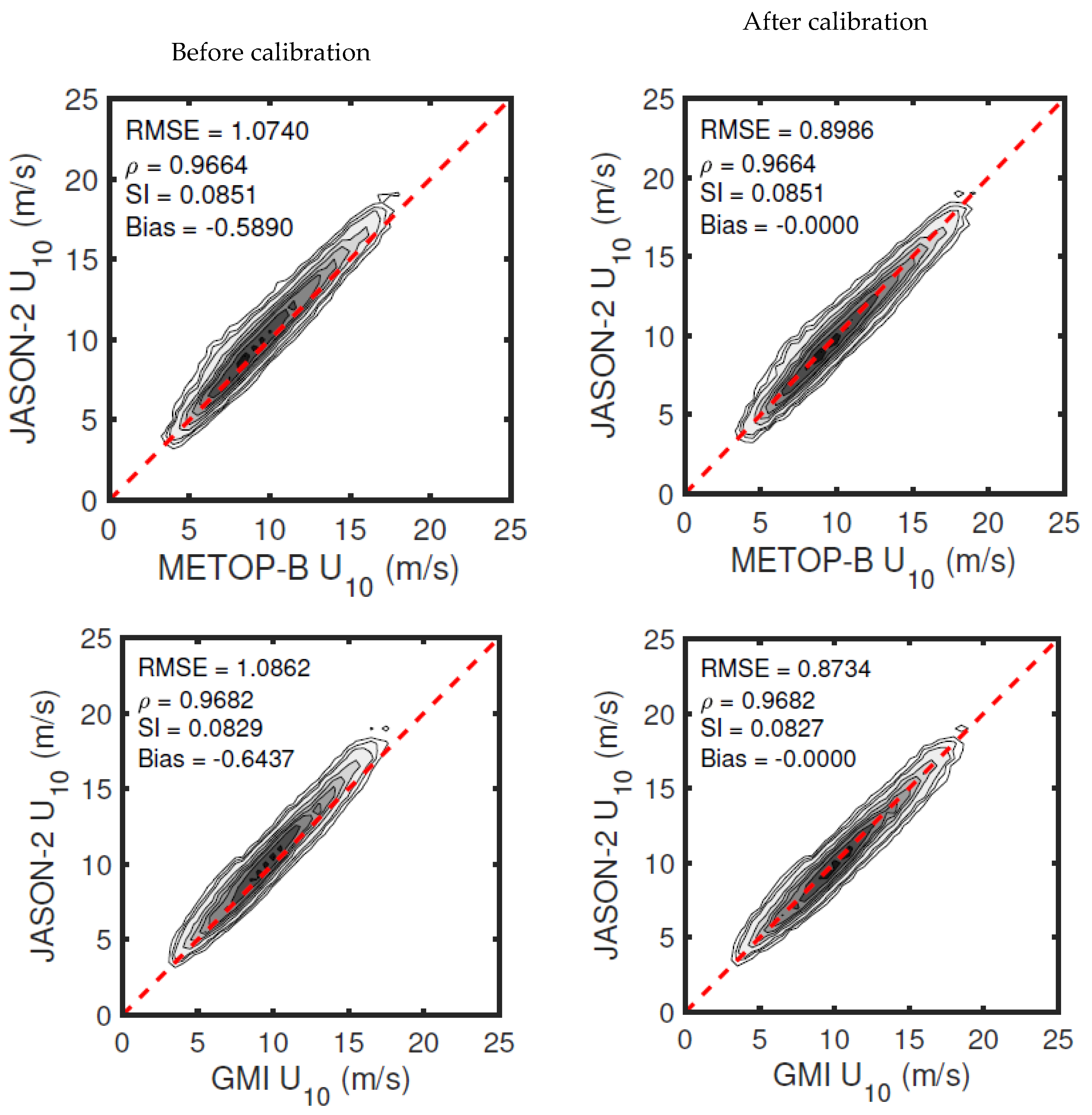
Figure 7 shows contour plots of data density for selected comparison cases, both before and after triple collocation calibrations were applied. As can be seen from the figure, although the correlation coefficients remain the same, there were changes in the values of RMSE, scatter index, and biases once the data are calibrated. As expected, the most significant change was bias, which is approximately zero after the calibrations relations were applied. This indicates that the calibration using triple collocation produces the expected outcomes.

5.2. Comparison of Calibration Approaches

As shown above, triple collocation and RMA regression produce very similar calibration relationships. However, there are some practical considerations which need to be taken into account when choosing a method.

If one is interested in estimating error variances, then triple collocation is the only available method to use. This is due to the fact that triple collocation can perform error estimations as well as calibration. However, as argued by Abdalla and Chiara [19], the method requires a few thousand collocated measurements to produce robust results. Therefore, most studies generally include a numerical model as one of the data sources for triple collocation. For example, METOP-B, CRYOSAT-2, and SSMI-F16 were operational at the same time but their respective orbits meant that there are no three-way matchups. In contrast, a huge number of matchups (more than 172,000) can be obtained if only two measurements are included such as METOP-B and CRYOSAT-2 or METOP-B and SSMI-F16. In this case, triple collocation is not a feasible solution.

Although reduced major axis (RMA) regression cannot be used to estimate error variances for a measurement, it also does not require a priori assumptions about the nature of the errors (e.g., uncorrelated random errors). Hence, RMA regression is a good solution if one is only interested in measurement calibration. It should be noted that neither approach will produce good results if the calibration is nonlinear, as has been noted at high wind speed. In such cases, a nonlinear or piecewise linear calibration can be applied [23,39].

6. Conclusions

Random error standard deviations of wind speed from 14 different measurement platforms have been estimated in the present work using triple collocation. The measurement platforms include six altimeters, three scatterometers, four radiometers, and NDBC buoys. Of all 13 satellite measurement systems, it is found that radiometers have the largest error standard deviations followed by scatterometers, with altimeters having the smallest error standard deviations. NDBC buoy data which is usually assumed as “ground truth” has error standard deviations larger than all the satellite systems. However, it is believed that the apparent low accuracy of the buoy is due to spatial representativeness errors.

Since triple collocation can simultaneously perform error estimation as well as calibration for a given reference, intercalibrations between satellites including NDBC buoy data have been carried out. Furthermore, calibration relations obtained from triple collocation have been compared with calibration relations obtained from reduced major axis (RMA) regression. It was found that the calibration relations obtained from the two approaches are very similar. Four different statistical parameters, namely RMSE, correlation coefficient, scatter index, and bias, have been evaluated and all show consistent results between the two calibration approaches.

The present work has not attempted to estimate error standard deviations for wind directions. Stoffelen [5] has qualitatively presented errors for wind direction for NDBC buoy data, not surprisingly showing that wind direction errors are larger at light winds. As only buoys and scatterometers measure wind direction, such an analysis could not be performed with the present datasets.

References

- Young, I.R.; Sanina, E.; Babanin, A.V. Calibration and cross validation of a global wind and wave database of altimeter, radiometer, and scatterometer measurements. J. Atmos. Ocean. Technol. 2017, 34, 1285–1306. [Google Scholar] [CrossRef]
- Verhoef, A.; Vogelzang, J.; Verspeek, J.; Stoffelen, A. Long-term scatterometer wind climate data records. IEEE J. Sel. Top. Appl. Earth Obs. Remote Sens. 2017, 10, 2186–2194. [Google Scholar] [CrossRef]
- Young, I.R.; Ribal, A. Multiplatform evaluation of global trends in wind speed and wave height. Science 2019, 364, 548–552. [Google Scholar] [CrossRef] [PubMed]
- Ribal, A.; Young, I.R. 33 years of globally calibrated wave height and wind speed data based on altimeter observations. Sci. Data 2019, 6, 77. [Google Scholar] [CrossRef] [Green Version]
- Stoffelen, A. Toward the true near-surface wind speed: Error modeling and calibration using triple collocation. J. Geophys. Res. Ocean. 1998, 103, 7755–7766. [Google Scholar] [CrossRef]
- An, R.; Zhang, L.; Wang, Z.; Quaye-Ballard, J.A.; You, J.; Shen, X.; Gao, W.; Huang, L.; Zhao, Y.; Ke, Z. Validation of the ESA CCI soil moisture product in China. Int. J. Appl. Earth Obs. Geoinf. 2016, 48, 28–36. [Google Scholar] [CrossRef]
- Draper, C.; Reichle, R.; de Jeu, R.; Naeimi, V.; Parinussa, R.; Wagner, W. Estimating root mean square errors in remotely sensed soil moisture over continental scale domains. Remote Sens. Environ. 2013, 137, 288–298. [Google Scholar] [CrossRef] [Green Version]
- Gruber, A.; Su, C.-H.; Zwieback, S.; Crow, W.; Dorigo, W.; Wagner, W. Recent advances in (soil moisture) triple collocation analysis. Int. J. Appl. Earth Obs. Geoinf. 2016, 45, 200–211. [Google Scholar] [CrossRef]
- Miyaoka, K.; Gruber, A.; Ticconi, F.; Hahn, S.; Wagner, W.; Figa-Saldana, J.; Anderson, C. Triple Collocation Analysis of Soil Moisture from Metop-A ASCAT and SMOS Against JRA-55 and ERA-Interim. IEEE J. Sel. Top. Appl. Earth Obs. Remote Sens. 2017, 10, 2274–2284. [Google Scholar] [CrossRef]
- Scipal, K.; Dorigo, W.; de Jeu, R. Triple collocation—A new tool to determine the error structure of global soil moisture products. In Proceedings of the International Geoscience and Remote Sensing Symposium, Honolulu, HI, USA, 25–30 July 2010; pp. 4426–4429. [Google Scholar]
- Su, C.H.; Ryu, D.; Crow, W.T.; Western, A.W. Beyond triple collocation: Applications to soil moisture monitoring. J. Geophys. Res. Atmos. 2014, 119, 6419–6439. [Google Scholar] [CrossRef]
- Van Dijk, A.I.J.M.; Renzullo, L.J.; Wada, Y.; Tregoning, P. A global water cycle reanalysis (2003–2012) merging satellite gravimetry and altimetry observations with a hydrological multi-model ensemble. Hydrol. Earth Syst. Sci. 2014, 18, 2955–2973. [Google Scholar] [CrossRef] [Green Version]
- Alemohammad, S.H.; McColl, K.A.; Konings, A.G.; Entekhabi, D.; Stoffelen, A. Characterization of precipitation product errors across the United States using multiplicative triple collocation. Hydrol. Earth Syst. Sci. 2015, 19, 3489–3503. [Google Scholar] [CrossRef] [Green Version]
- Thao, S.; Eymard, L.; Obligis, E.; Picard, B. Trend and variability of the atmospheric water vapor: A mean sea level issue. J. Atmos. Ocean. Technol. 2014, 31, 1881–1901. [Google Scholar] [CrossRef] [Green Version]
- Ratheesh, S.; Mankad, B.; Basu, S.; Kumar, R.; Sharma, R. Assessment of satellite-derived sea surface salinity in the Indian ocean. IEEE Geosci. Remote Sens. Lett. 2013, 10, 428–431. [Google Scholar] [CrossRef]
- Caires, S.; Sterl, A. Validation of ocean wind and wave data using triple collocation. J. Geophys. Res. Ocean. 2003, 108, 1–16. [Google Scholar] [CrossRef]
- Janssen, P.A.E.M.; Abdalla, S.; Hersbach, H.; Bidlot, J.-R. Error estimation of buoy, satellite, and model wave height data. J. Atmos. Ocean. Technol. 2007, 24, 1665–1677. [Google Scholar] [CrossRef] [Green Version]
- Chakraborty, A.; Kumar, R.; Stoffelen, A. Validation of ocean surface winds from the OCEANSAT-2 scatterometer using triple collocation. Remote Sens. Lett. 2013, 4, 85–94. [Google Scholar] [CrossRef]
- Abdalla, S.; Chiara, G.D. Estimating random errors of scatterometer, altimeter, and model wind speed data. IEEE J. Sel. Top. Appl. Earth Obs. Remote Sens. 2017, 10, 2406–2414. [Google Scholar] [CrossRef]
- McColl, K.A.; Vogelzang, J.; Konings, A.G.; Entekhabi, D.; Piles, M.; Stoffelen, A. Extended triple collocation: Estimating errors and correlation coefficients with respect to an unknown target. Geophys. Res. Lett. 2014, 41, 6229–6236. [Google Scholar] [CrossRef] [Green Version]
- Wu, X.; Xiao, Q.; Wen, J.; You, D. Direct comparison and triple collocation: Which is more reliable in the validation of coarse-scale satellite surface albedo products. J. Geophys. Res. Atmos. 2019, 124, 5198–5213. [Google Scholar] [CrossRef]
- Vogelzang, J.; Stoffelen, A. Triple Collocation. NWPSAF Technical Report NWPSAF-KN-TR-021 2012, EUMETSAT. Available online: http://projects.knmi.nl/publications/fulltexts/triplecollocation_nwpsaf_tr_kn_021_v1.0.pdf (accessed on 22 July 2019).
- Ribal, A.; Young, I.R. Calibration and cross-validation of global ocean wind speed based on scatterometer observation. J. Atmos. Ocean. Technol. 2020, 37, 279–297. [Google Scholar] [CrossRef]
- Vogelzang, J.; Stoffelen, A.; Verhoef, A.; Figa-Saldaña, J. On the quality of high-resolution scatterometer winds. J. Geophys. Res. Ocean. 2011, 116, C10033. [Google Scholar] [CrossRef] [Green Version]
- Harper, W.V. Reduced major axis regression: Teaching alternatives to least squares. In Proceedings of the Ninth International Conference on Teaching Statistics (ICOTS9), Flagstaff, AZ, USA, 13–18 July 2014. [Google Scholar]
- Holland, P.W.; Welsch, R.E. Robust regression using iteratively reweighted least-squares. Commun. Stat. Theory Methods 1977, 6, 813–827. [Google Scholar] [CrossRef]
- Chelton, D.B.; Ries, J.C.; Haines, B.J.; Fu, L.L.; Callahan, P.S. Satellite Altimetry. In Satellite Altimetry and Earth Sciences: A Handbook of Techniques and Applications; Fu, L.-L., Cazenave, A., Eds.; Academic Press: San Diego, CA, USA, 2001; Volume 69, pp. 1–131. [Google Scholar]
- Abdalla, S. Ku-band radar altimeter surface wind speed algorithm. Mar. Geod. 2012, 35, 276–298. [Google Scholar] [CrossRef] [Green Version]
- Mears, C.A.; Smith, D.K.; Wentz, F.J. Comparison of special sensor microwave Imager and buoy-measured wind speeds from 1987 to 1997. J. Geophys. Res. Ocean. 2001, 106, 11719–11729. [Google Scholar] [CrossRef] [Green Version]
- Hollinger, J.P.; Peirce, J.L.; Poe, G.A. SSM/I instrument evaluation. IEEE Trans. Geosci. Remote Sens. 1990, 28, 781–790. [Google Scholar] [CrossRef]
- Wentz, F.J. A well-calibrated ocean algorithm for special sensor microwave / imager. J. Geophys. Res. Ocean. 1997, 102, 8703–8718. [Google Scholar] [CrossRef] [Green Version]
- Meissner, T.; Wentz, F.J. The emissivity of the ocean surface between 6 and 90 GHz over a large range of wind speeds and earth incidence angles. IEEE Trans. Geosci. Remote Sens. 2012, 50, 3004–3026. [Google Scholar] [CrossRef]
- Takbash, A.; Young, I.R. Global ocean extreme wave heights from spatial ensemble data. J. Clim. 2019, 32, 6823–6836. [Google Scholar] [CrossRef]
- Priestley, C.H.B. Turbulent Transfer in the Lower Atmosphere; University of Chicago Press: Chicago, IL, USA, 1959. [Google Scholar]
- Young, I.R. Seasonal variability of the global ocean wind and wave climate. Int. J. Climatol. 1999, 19, 931–950. [Google Scholar] [CrossRef]
- Zieger, S.; Vinoth, J.; Young, I.R. Joint calibration of multiplatform altimeter measurements of wind speed and wave height over the past 20 years. J. Atmos. Ocean. Technol. 2009, 26, 2549–2564. [Google Scholar] [CrossRef]
- Nearing, G.S.; Yatheendradas, S.; Crow, W.T.; Bosch, D.D.; Cosh, M.H.; Goodrich, D.C.; Seyfried, M.S.; Starks, P.J. Nonparametric triple collocation. Water Resour. Res. 2017, 53, 5516–5530. [Google Scholar] [CrossRef]
- Zieger, S.; Babanin, A.V.; Erick Rogers, W.; Young, I.R. Observation-based source terms in the third-generation wave model WAVEWATCH. Ocean. Model. 2015, 96, 2–25. [Google Scholar] [CrossRef] [Green Version]
- Takbash, A.; Young, I.R.; Breivik, Ø. Global wind speed and wave height extremes derived from long-duration satellite records. J. Clim. 2019, 32, 109–126. [Google Scholar] [CrossRef]
Figure 1.
Durations of all satellite data used for the present analysis.
Figure 2.
Locations of the NODC buoys (blue stars) used in this study where only buoys more than 50 km offshore are used.
Figure 3.
Error standard deviations, , (m/s) per year for (a) TOPEX, QUIKSCAT, and SSMI-F15; (b) JASON-1, QUIKSCAT, and SSMI-F15; (c) The number of matchups used per year for the case (a); (d) The number of matchups used per year for the case (b). The results in (a) and (b) show that the error standard deviations are approximately constant over time, a requirement of the triple collocation approach.
Figure 4.
Calibration of METOP-A wind speed against National Data Buoy Center (NDBC) buoy data using reduced major axis (RMA) and triple collocation. The contours represent the normalized density of data points, with contours drawn at 0.9, 0.7, 0.5, …, 0.1, 0.07, 0.04 (maximum value is one). Dots represent outliers excluded from RMA regression using robust regression. refer to calibrated values of wind speed and to uncalibrated values. n and nout are the number of clean (i.e., not outliers) collocated measurements and the number of outliers, respectively.
Figure 5.
Calibration of WINDSAT wind speed against NDBC buoy data using RMA and triple collocation. The contours represent the normalized density of data points, with contours drawn at 0.9, 0.7, 0.5, …, 0.1, 0.07, 0.04 (maximum value is one). Dots represent outliers excluded from RMA regression using robust regression. refer to calibrated values of wind speed and to uncalibrated values. n and nout are the number of clean (i.e., not outliers) collocated measurements and the number of outliers, respectively.
Figure 6.
Calibration of METOP-A wind speed with respect to WINDSAT using RMA and triple collocation. The contours represent the normalized density of data points, with contours drawn at 0.9, 0.7, 0.5, …, 0.1, 0.07, 0.04 (maximum value is one). Dots represent outliers excluded from RMA regression using robust regression. refer to calibrated values of wind speed and to uncalibrated values. n and nout are the number of clean (i.e., not outliers) collocated measurements and the number of outliers, respectively.
Figure 7.
Comparisons of selected cases of matchup data before and after triple collocation calibrations were applied. The contours represent the normalized density of data points, with contours drawn at 0.9, 0.7, 0.5, …, 0.1, 0.07, 0.04 (maximum value is one).