The Fusion of Spectral and Structural Datasets Derived from an Airborne Multispectral Sensor for Estimation of Pasture Dry Matter Yield at Paddock Scale with Time

Abstract

This study aimed to develop empirical pasture dry matter (DM) yield prediction models using an unmanned aerial vehicle (UAV)-borne sensor at four flying altitudes. Three empirical models were developed using features generated from the multispectral sensor: Structure from Motion only (SfM), vegetation indices only (VI), and in combination (SfM+VI) within a machine learning modelling framework. Four flying altitudes were tested (25 m, 50 m, 75 m and 100 m) and based on independent model validation, combining features from SfM+VI outperformed the other models at all heights. However, the importance of SfM-based features changed with altitude, with limited importance at 25 m but at all higher altitudes SfM-based features were included in the top 10 features in a variable importance plot. Based on the independent validation results, data generated at 25 m flying altitude reported the best model performances with model accuracy of 328 kg DM/ha. In contrast, at 100 m flying altitude, the model reported an accuracy of 402 kg DM/ha which demonstrates the potential of scaling up this technology at farm scale. The spatial-temporal maps provide valuable information on pasture DM yield and DM accumulation of herbage mass over the time, supporting on-farm management decisions.

1. Introduction

With numerous challenges facing the dairy sector in Australia, optimising the utilisation of home-grown pasture, the cheapest feed, is an essential target for the sustainability and profitability of the industry [1,2,3]. Emerging technologies such as virtual fencing can only be effectively implemented with accurate and timely information on feed resources across a given area (i.e., paddock-scale). State-of-the-art sensor technologies offer new opportunities for measuring and managing pasture dry matter (DM) yield within paddock and across farms in near-real-time through characterisation of its variability in space-time.

Predicting spatial variability of pasture DM yield and nutritive characteristics across farms is challenging due to heterogeneous pasture accumulation patterns; the impact of management decisions, such as grazing and species heterogeneity; and the effect of other factors such as terrain and variable soil types as all affect pasture production in a landscape context [4]. Traditionally, estimation of DM yield at a paddock or farm-scale is undertaken through developed allometric equations derived through empirical relationships between the pasture DM yield and sward height [5]. For instance, the rising plate meter (RPM) provides average paddock-scale estimates via calibrated equations to predict pasture DM yield [6,7]. However, these approaches ignore the spatial variability of pasture DM yield across the paddock resulting in under or over utilisation of this feed resource. Past work has shown the ability to utilise different sensor technologies, such as (a) proximal sensing (e.g., ground-based sonar [8], active multi-spectral sensors [9] or a combination of active and LiDAR sensors mounted on farm vehicles [10]), (b) aerial sensors [11,12] and (c) satellite-based technologies [13,14] to provide estimates of pasture DM yield. Nevertheless, practical applications of these technologies on-farm are limited due to many factors such as associated driving time for data collection for large paddocks using vehicle-mounted proximal sensors, and coarse spatial resolution of satellite-derived datasets as well as the impact of clouds on data quality when utilising passive remote sensing products.

The Australian dairy industry relies on a predominantly grazing-based system. Land managers are interested in not only the pre-grazing pasture DM yield, but also the post-grazing residual as these two factors determine the amount consumed by the cow and can equally influence longer term pasture productivity and persistence. In addition, the height and evenness of post-grazing residual is an important factor for pasture recovery rate. To capture such DM yield variability, it is essential to develop robust models that can predict pasture DM yield across the paddock and over time. Previous studies associated with UAV-borne sensor technologies have generally focussed on measurements closer to grazing. These studies are based mostly within European temperate agriculture production systems [11,12]. Furthermore, these production systems are mainly targeted at optimising the harvest of conserved forage (i.e., hay and silage) to provide feed for indoor dairy systems. This requires a very different approach to pasture management than that of the large-scale and intensive rotationally grazed pasture-based systems that are more commonly used in the Australian dairy industry.

There is untapped potential to utilise rich datasets gathered through Unmanned Aerial Vehicle (UAV)-borne systems for measurement and subsequent management of pasture production systems. These UAV-borne systems provide very high-resolution datasets at the paddock scale and have other advantages over passive remote sensing systems such as satellite datasets, fewer issues with atmospheric correction and removing the impact of clouds on data availability. Quantification of biomass using UAV-associated technologies is not new. There has been a great deal of work associated with quantification of crop biomass over the last decade using UAV-derived datasets [15,16,17]. In comparison to crop production systems, grazing production systems do not have the luxury of synchronised continuous growth and harvest, where the latter is often disturbed through intermediate grazing or cutting herbage for forage conservation. As such, spatial-temporal modelling of pasture DM yield at the paddock scale is far more challenging.

Both spectral and structural (e.g., height) characteristics of pasture are important for the prediction of pasture DM yield [11,12,18]. Spectral information can be gathered through different sensors, including RGB [19], multispectral [4,20] or hyperspectral [21] instruments. These spectral datasets are then processed to derive vegetation indices (VI; e.g., Normalised Difference Vegetation Index) that are used as drivers for the development of empirical relationships between measured pasture DM yield [18,22]. There is also a growing interest in utilising three-dimensional (3D) datasets gathered through UAV-borne remote sensing platforms for pasture DM modelling. These 3D datasets can be effectively re-arranged to derive a variety of features (covariates) to represent the crop surface model (CSM) across the landscape which then act as a proxy for plant structural components such as height [11]. These 3D structures can be created from (a) UAV-mounted active sensors through direct measurement of the distance between the object and the sensor (e.g., LiDAR) or (b) through further processing of 2D images acquired using a passive sensor [11]. For the latter, state-of-the-art passive algorithms such as Structure from Motion (SfM) are commonly used to generate 3D datasets from 2D images. Previous studies [11,23,24] provide some early results on the usage of SfM datasets to successfully model pasture DM yield.

There is a growing trend to simultaneously use both structural and spectral information for modelling of pasture DM yield especially in the area of high-throughput phenotyping (HTP) applications where experiments are typically carried out at small plot scale [20]. However, there are few studies that have focused on modelling pasture DM yield within farm or at the paddock scale using both structural and spectral characteristics simultaneously, rather, previous work of this kind has focussed on small extents and has not tested the ability to scale up technologies to commercial farm-scale applications [11]. Scaling up these methodologies to landscape-scale is currently constrained by UAV battery life, data processing speed and by a lack of automated data processing pipelines. Furthermore, the effects of flying at different altitudes on pasture DM model prediction quality (model performances) needs to be better understood to develop best practice guidelines for the use of UAVs for on-farm application and to prepare for future technology improvements. This study aimed to (a) evaluate the prediction quality of models derived from structural information only, spectral information only or a combination of structural and spectral information, obtained from UAV-borne datasets; (b) test the effect of different flying altitudes on model quality; and finally (c) use the derived models to produce estimates of paddock-scale spatial-temporal variability of pasture DM yield. It is anticipated that these spatial-temporal variability maps can be used for optimising on-farm feed utilisation.

2. Materials and Methods

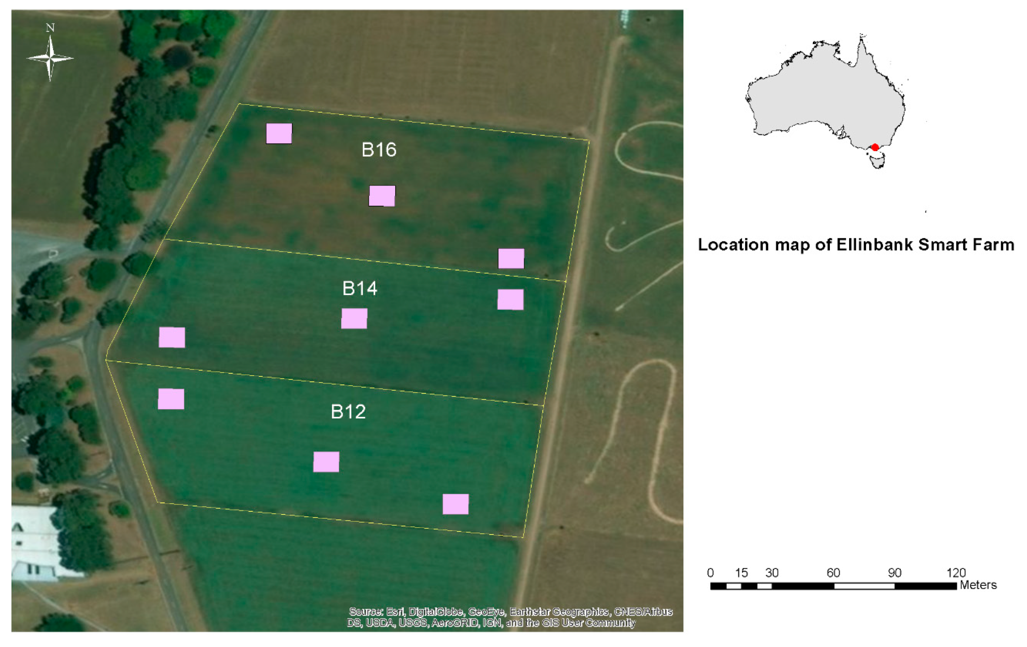
2.1. Study Area

Data collection was carried out between October and November 2019 over 3 adjacent paddocks, which covered a total area of 3.02 ha (hereafter known as B’s and consisted of sub-paddocks B12, B14 and B16) at the Ellinbank Smart Farm (38.2408 S, 145.9414 E), Agriculture Victoria, Australia (Figure 1). The topography of the paddocks varies from the 155 m to 177 m. The sub-paddocks were chosen to encompass sufficient spatial variation to enable training of robust spatial-temporal models. The paddocks were previously sown with perennial ryegrass (Lolium Perenne L. PRG), with additional over-sowing of PRG in March 2019. The paddocks were cut for silage on 1st October 2019 at approximately 5 cm above ground-level using a tractor-mounted mower to provide a uniform pasture height, and an inorganic nitrogen-based fertiliser was applied (33.6 kg N/ha) (

Table 1. Summary of agronomic practices applied and field sampling campaigns and associated UAV survey missions.

Management Activity/Measurement	Date
Cut for silage	1 October 2019
Fertiliser applied	4 October 2019
Baseline week	10 October 2019
Measurement week 1	14 October 2019
Measurement week 2	22 October 2019
Measurement week 3	28 October 2019
Measurement week 4	5 November 2019

). Four temporal measurements were taken following silage and prior to the next grazing event, at approximately weekly intervals (Table 1). Weekly measurements aimed to capture the heterogeneous nature of pasture DM accumulation across the landscape and with time enabling the development of a spatial and temporal empirical model to predict pasture DM yield at farm scale.

2.2. Sampling Design and Field Data Collection

Three pre-identified 10 m × 10 m spatial resolution units (henceforth termed “pixels” as they match the spatial grids of the Sentinel 2 satellite) within each of the sub-paddocks were chosen which resulted total of nine pixels (Figure 1). This ensured that samples were collected across the area of interest, covered the spatial extent and met the logistical requirements of field data collection. The sampling scheme employed in the current study was considered a stratified random sampling scheme. Each pixel was considered as a stratum, and three independent samples (at each measurement) were randomly collected within the pixel using a 35 cm × 70 cm quadrat. The three sampling locations within each pixel were randomised by following a set of predetermined bearings and positions for each timepoint, thus removing subjectivity and preventing double-sampling of the same area.

The quadrat was considered as the primary unit for model calibration with their positions and attributes recorded using the ESRI Collector^TM application. The Collector app was used to record measurements within the quadrat polygon defined using an EMLID Reach RS+ GPS unit set-up in RTK mode with a horizontal accuracy of +/−7 mm and vertical accuracy of +/−14 mm (Emlid Ltd., Australia). Finally, destructive sampling of the pasture was undertaken in the area covered by the quadrat using battery-powered hand shears. As the overall research program, of which this study formed a part, was aimed at predicting both pasture nutritive characteristics (reported separately) and quantity, each sample was cut in two portions where the top portion, represented the biomass available for grazing, and underwent additional nutritional analysis as well as for dry matter yield determination.

In brief, biomass greater than 5 cm and the remaining biomass between 5 cm and the ground were cut separately. The >5 cm sample was sub-divided into 25% and 75% portions using a quartering technique. Fresh weights of each subsample were recorded. The 25% subsample was oven-dried at 100 °C until a constant weight was obtained to determine DM percentage and applied to the total weight of the >5 cm fraction. Samples cut at less <5 cm were first washed to remove any contamination during field data collection and then dried at 100 °C following the same procedure until a constant weight was obtained. Total pasture DM yield was calculated as the cumulative dry matter yield value for the two samples. For modelling and reporting purposes, the pasture DM yield in each quadrat was converted to a kg DM/ha basis.

2.3. Acquisition of UAV-Borne Datasets

A DJI M200 (DJI Technology Co., Shenzhen, China) UAV, which was equipped with a RedEdge-MX (MicaSense Inc., Seattle, WA, USA) multispectral sensor, was used to collect the aerial datasets. All mission paths were designed to fly using a single grid pattern with 25 m, 50 m, 75 m and 100 m flying altitudes. A summary of the missions is depicted in

Table 2. The summary of the flying mission carried out at varying flying altitudes.

Flight Altitude (m)	Forward Overlap (Speed)	Side Overlap	Ground Sampling Distance (GSD)
25	80% (3.2 m/s)	80%	1.74 cm/pixel
50	80% (6.5 m/s)	80%	3.47 cm/pixel
75	80% (10 m/s)	80%	5.21 cm/pixel
100	80% (13 m/s)	80%	6.94 cm/pixel

. All mission data collections were carried out between 1100 h and 1300 h. The sensor characteristics of RedEdge-MX multispectral sensor are shown in

Table 3. Summary of the spectral and spatial characteristics of the MicaSense RedEdge-MX sensor.

Band	Spectral Resolution (nm)	Resolution (px)
Blue	465–485	1200 × 960
Green	550–570	1200 × 960
Red	663–673	1200 × 960
Red Edge	712–722	1200 × 960
NIR	820–860	1200 × 960

. During the flight mission, ground calibration tarpaulins with known reflection values of 3%, 6%, 11%, 22%, 33%, and 44% were laid on the ground for radiometric calibration of the acquired multispectral datasets for ground reflectance.

2.4. Processing of UAV Datasets and Deriving Structural and Spectral Features

2.4.1. Preprocessing of the UAV-Derived Datasets

Pix4D Mapper Pro (version 4.3.31 Pix4D, Lausanne, Switzerland) was used to process images. A customised “AgMultispectral” settings template was used to process acquired datasets including geometric corrections using 3D ground control points (GCPs) (n = 10) through realignment in the X, Y and Z axes and re-optimisation. The GCPs were marked using an EMLID Reach RS+ GPS unit setup in RTK mode. Automatic tie points were used for densification and classification of the generated 3D point cloud through the SfM algorithm embedded within the Pix4D software. Finally, for each survey, a digital surface model (DSM), digital terrain model (DTM), orthomosaic images with raw digital numbers (DN) (for each of the five bands), and point cloud data were exported from the Pix4D software.

As previously described [20], orthomosaic images were calibrated using empirical line calibration method using the ground calibration tarpaulins with known reflectance values. To summarise this process, the orthomosaic bands were first loaded into the QGIS Version 3.4.2-Madeira (QGIS Development Team, 2017, Raleigh, NC, USA) environment. The calibration tarpaulin areas were manually digitised into polygons, and the known reflectance panel percentage was entered as the polygon unique identification number. Then, within QGIS, the zonal statistics tool was used to extract the mean value of the raw DN within each polygon for each of the five corresponding bands acquired though the MicaSense Red Edge MX sensor. Extracted data were regressed against the known reflectance and the obtained regression equation was used to convert the image’s raw DN to surface reflectance.

2.4.2. Evaluation of the Accuracy of the SfM Z Estimates

The accuracy of the reported Z values within the point cloud dataset was evaluated with known Z (elevation) obtained using an EMLID Reach RS+ RTK-GPS unit. Artificial height references (AHR), each consisting of a group of seven boxes with flat, levelled, surfaces (0.5 m × 0.5 m), were placed at the top and bottom of the paddock across the slope (Supplementary Material; Figure S2). Centres of each AHR were marked using RTK GPS resulting in a total of 14 AHRs. A circular buffer of 20 cm diameter was created in a GIS environment around the centre-point (X and Y) of the AHR and SfM data within the buffer zone were extracted. Having a buffer of 20 cm ensured that only the SfM data that was known to be within the 0.5 × 0.5 m AHR structures were extracted for further evaluation. The mean and standard deviation values for SfM Z were calculated for each of the 14 AHRs. The error associated with SfM Z was determined by the difference between the SfM Z and the RTK GPS Z. Results from this analysis were not the main focus of this manuscript but are included as supplementary material used to support the discussion (Supplementary material; Figures S1 and S2).

2.4.3. Deriving Structural and Spectral Features

Pasture height (PH) (CSH—crop surface height) was derived for all quadrats using an approximated baseline digital terrain model (DTM) or digital surface model (DSM) and using the point cloud data generated for each measurement survey period (Equation (1)).

Z_{CSH for x}^th _location = Z _{for x}^th_location − Z_{DSM or DTM of the baseline survey}

(1)

A proxy for a DTM was used. This was due to the difficulty in observing any bare surface in the pasture after mechanical harvesting and the pasture accumulation in the following two weeks was small and difficult to measure. As previously explained the cutting height used in the mechanical harvesting process was approximately 5 cm, after one week of growth the PH was approximated at 7 cm and therefore a standardised offset of 7 cm was applied to baseline DSM to approximate ground level. Therefore, the structural characteristics of the pasture canopy were calculated using Equation (2).

Z_{CSH for x}^th _location = Z _{for x}^th _location − Z_{DSM of the baseline survey − 7 cm offset}

(2)

Results from Equation (2) were filtered for any unrealistic values by removing values > 1 m and negative values. This resulted in a total of 101 usable polygons out of a possible 108, used for model development and validation purposes. Additional features were derived for each quadrat, including mean, minimum, maximum and the quantiles 0.05, 0.10. 0.25, 0.50, 0.75, 0.90, and 0.95 to represent surrogates for PH.

A variety of VIs and individual spectral bands were derived using the calibrated orthomosaic images. These spectral datasets were generated using ENVI software Version 5.5 through model builder (Exelis Visual Information Solutions, Boulder, CO, USA). The key VIs derived from the multispectral images are summarised in

Table 4. The summary of the key indices derived from spectral and structure from motion datasets.

Name	Abbreviation	Equation	Reference
Blue reflectance band	Mean_X5band_T.1
Green reflectance band	Mean_X5band_T.2
Red reflectance band	Mean_X5band_T.3
Red Edge reflectance band	Mean_X5band_T.4
Near Infrared reflectance band	Mean_X5band_T.5
Normalised Difference Vegetation Index	Mean_NDVI_T	(NIR − R)/(NIR + R)	Rouse et al. (1973) [25]
Green Normalised Difference Vegetation Index	Mean_GNDVI_T	(NIR − G)/(NIR + G)	Gitelson et al. (1996) [26]
Red Edge Normalised Difference Vegetation Index	Mean_ReNDVI_T	(NIR − RE)/(NIR + RE)	Gitelson and Merzlyak (1994) [27]
Red Edge Simple Ratio	Mean_ReSRI_T	NIR/RE	Gitelson et al. (2005) [28]
Enhanced Vegetation Index 2	Mean_EVI2_T	2.5 × (NIR − R)/(NIR + (2.4 × R) + 1)	Huete et al. (2002) [29]
Green Chlorophyll Index	Mean_GCI_T	(NIR/G) − 1	Gitelson et al. (2005) [28]
Red Edge Chlorophyll Index	Mean_ReCI_T	(NIR/RE) − 1	Gitelson et al. (2005) [28]
Medium Resolution Imaging Spectrometer (MERIS) Terrestrial Chlorophyll Index (MRCI)	Mean_MRCI_T	(NIR − RE)/(RE + R)	Dash and Curran (2004) [30]
Core Red Edge Triangular Vegetation Index	Mean_CReTVI_T	100(NIR − RE) − 10(NIR − G)	Chen et al. (2010) [31]
Red Difference Index	Mean_RedDI_T	NIR − R	Tucket (1979) [32]
Canopy Chlorophyll Concentration Index	Mean_CCCI_T	((NIR − RE)/(NIR + RE))/NDVI	Jago et al. (1999) [33]
Green Difference Index	Mean_GreenDI_T	NIR − G	Sripada (2005) [34]
Green Ratio Simple Index	Mean_GRSI_T	NIR/G	Sripada et al. (2006) [35]
Soil Adjusted Vegetation Index	Mean_SAVI_T	((NIR − R)/(NIR − R + 0.5)) ∗ (1 + 0.5)	Huete (1988) [36]
Anthocyanin Reflectance Index 1	Mean_ARI1_T	(1/G) − (1/RE)	Gitelson et al. (2007) [37]
SfM height − minimum	min
SfM height − maximum	max
SfM height − mean	mean
SfM height − Quantile − 0.05	p05
SfM height − Quantile − 0.10	p10
SfM height − Quantile − 0.25	p25
SfM height − Quantile − 0.50	p50
SfM height − Quantile − 0.75	p75
SfM height − Quantile − 0.90	p90
SfM height − Quantile − 0.95	p95

.

2.5. Data Modelling

A Random Forest model was used to determine the features of greatest influence in predicting pasture DM yield as it has the ability to handle both linear and nonlinear relationships and the presence of multicollinearity among the input features. The Random Forest modelling approach is an ensemble learning method and detail on the algorithm is provided in Brieman (2001) [38]. In the current study, the “ranger” package in the software R was used to create the model, which is a fast implementation of Random Forest for high dimensional data [39]. Prior to modelling at each of the different flying altitudes, a Pearson’s correlation matrix was produced to examine the relationships between the features within the dataset and measured pasture DM yield.

The dataset was split into calibration (80%) (n = 81) and validation (20%) (n = 20) using a conditional Latin hypercube sampling (cLHC) strategy [40], where (a) individual pixels within each sub-paddock area (i.e., B12, B14 and B16) and (b) measured pasture DM yield were used as inputs for the cLHC sampling algorithm. Latin hypercube sampling is a procedure that provides an efficient way of sampling variables from their multivariate distributions using a stratified random approach. It enables a full coverage of the range of each variable to be selected by maximally stratifying the marginal distribution. The same calibration and validation datasets were developed for all models at all flying altitudes. This enabled inter-model comparison to be undertaken.

Three types of models were fitted: (a) structural information only ((SfM), (b) spectral information only (VI) and (c) a combination of structural and spectral information (SfM+VI). Each model was optimised for key Random Forest model hyperparameters (mtry, n-nodes, variance type) through 10-fold cross-valuation techniques. Once the optimum model hyperparameters were obtained, those models were validated using two approaches (a) leave-one-out cross-validation (LOOCV) and (b) fully independent validation.

Model quality was assessed using (a) root mean squared error (RMSE) as a measure of model accuracy, (b) normalised RMSE and (c) Lin’s concordance correlation (LCC), which measures the variation of predicted values from a 45-degree line (1:1 line) in a validation plot [41]. The best model was selected considering the lowest RMSE and highest LCC out of the three types of models for each flying altitude. These validation indices were calculated as below,

$$\mathrm{RMSE}={\displaystyle \sum }_{i=1}^N\frac{{(\mathrm{Y}-\mathrm{Yi})}^2}{N}$$

(3)

where $\mathrm{Y}$ = Observed pasture DM yield value, $\mathrm{Yi}$ = Predicted pasture DM yield value and N is the number of samples.

$$\begin{array}{cc}\mathrm{Normalise}\mathrm{RMSE}& =\mathrm{RMSE}\times 100\hfill \\ & \mathrm{Mean}\mathrm{measured}\mathrm{pasture}\mathrm{DM}\mathrm{yield}\hfill \end{array}$$

(4)

The LCC can be defined as

$$\mathrm{LCC}=\frac{2{\mathsf{\rho }\mathsf{\sigma }}_{\mathrm{x}}{\mathsf{\sigma }}_{\mathrm{y}}}{{\mathsf{\sigma }}_{\mathrm{x}}^2+{\mathsf{\sigma }}_{\mathrm{y}}^2+{\left({\mathsf{\mu }}_{\mathrm{x}}-{\mathsf{\mu }}_{\mathrm{y}}\right)}^2}$$

(5)

where μ_x and μ_y are the means for the measured and predicted pasture DM yield, ${\mathsf{\sigma }}_{\mathrm{x}}^2$ and ${\mathsf{\sigma }}_{\mathrm{y}}^2$ are the corresponding variances of measured and predicted pasture DM yield and ρ is the Pearson correlation coefficient between the measured and predicted pasture DM yield. Even though the model quality evaluation in this manuscript is based on the above three model quality indices, most published work reported model evaluation based on coefficient of determination (R²); therefore, for the purpose of comparison, additional validation indices were calculated including mean error (ME) as a measure of model bias, Pearson’s correlation (r) and R². A summary of this analysis is included in the supplementary material (Tables S1 and S2).

In order to assess statistical significance, the prediction bias (Measured–Predicted) was contrasted for each validation datapoint within each tested model against each other using linear mixed models. In the linear mixed model, the model type was considered as a fixed effect term and sampling quadrat location was considered as a random effect which accounted for unknown variability. Mean separation was conducted using the LSD mean separation technique at the 0.05 probability level.

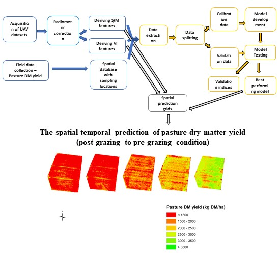
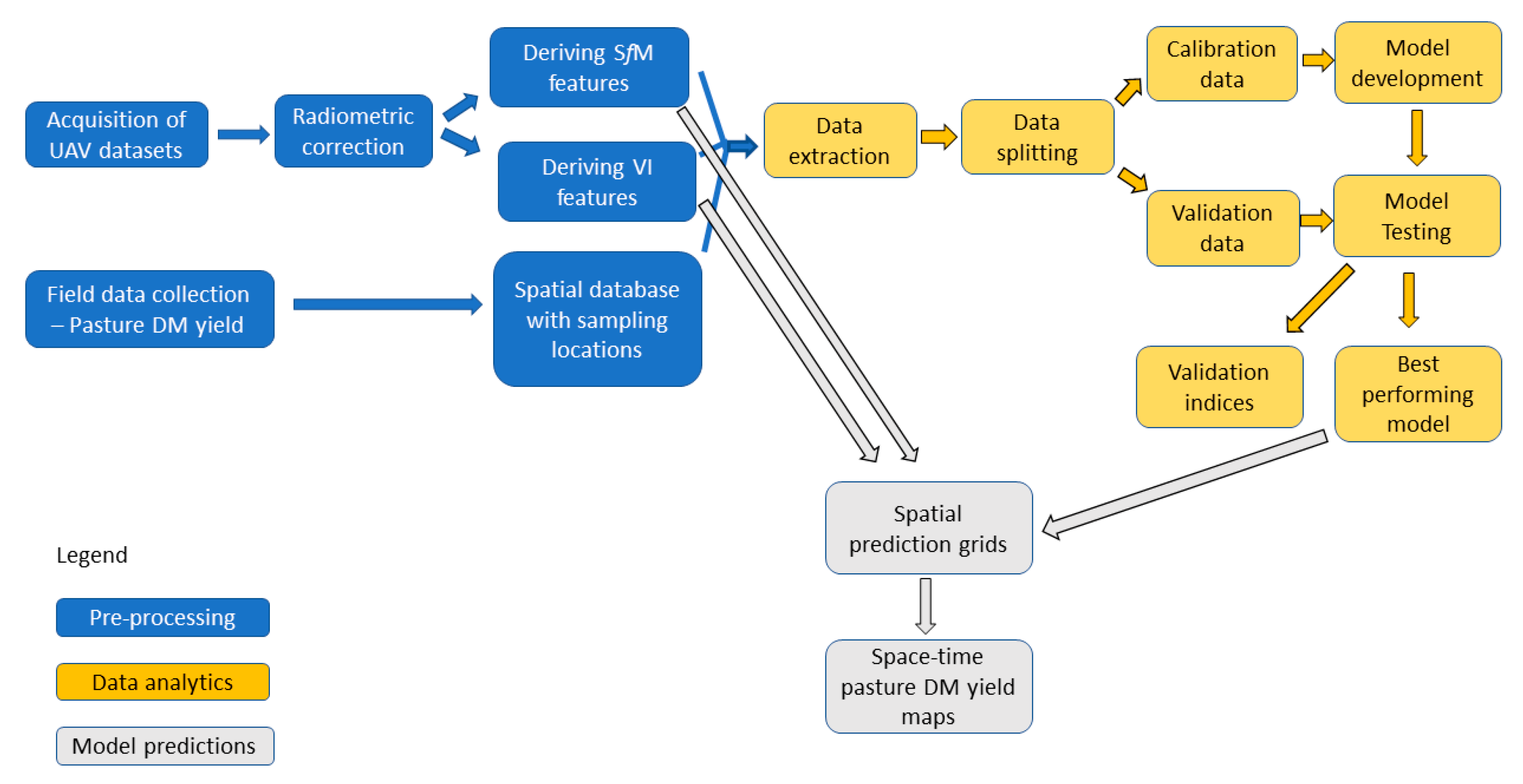
2.6. Spatial-Temporal Predictions across the Landscape

Space-time prediction across the landscape was implemented at a 1 m spatial resolution. The spectral data were resampled to 1 m resolution using a bilinear interpolation method and SfM data were summarised onto a 1 m grid prior to carrying out the prediction. The graphical summary of the methodology adopted for data modelling (analysis approach) is depicted in Figure 2.

3. Results

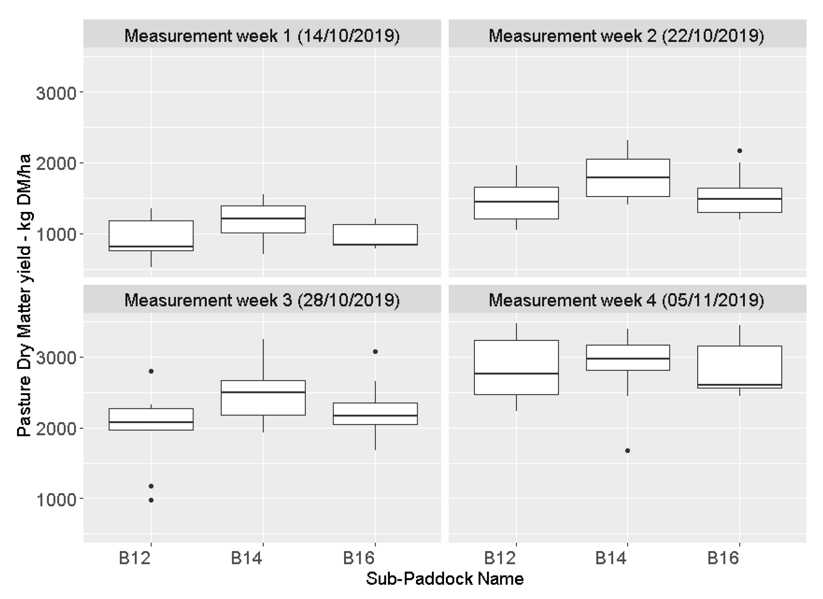
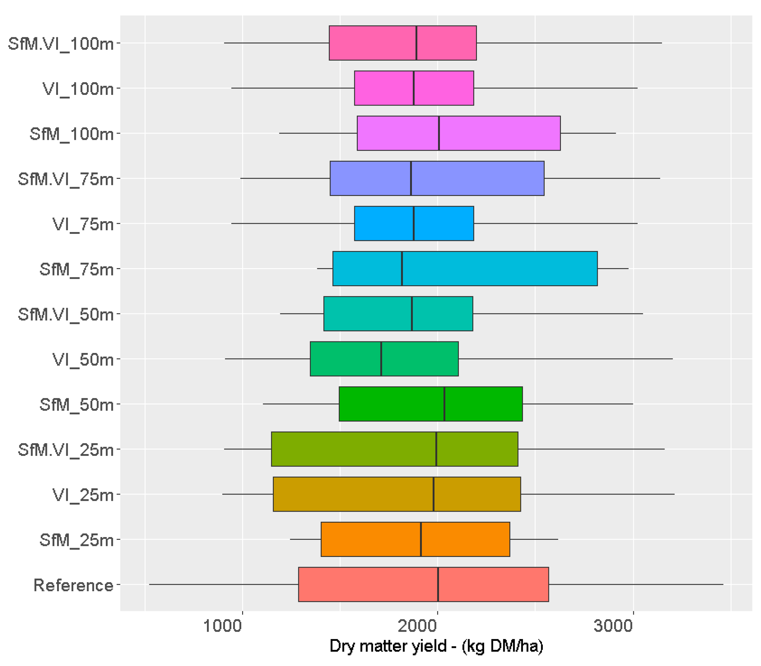
3.1. Temporal Variation of Pasture Dry Matter Yield

The mean pasture DM yields for the B paddocks were reported as 1013 kg DM/ha (±285 s.d.), 1596 kg DM/ha (±347 s.d.), 2223 kg DM/ha (±502 s.d.) and 2843 kg DM/ha (±447 s.d.) for measurement (sampling) weeks 1–4 respectively. Mean DM yield and its distribution measurement across the three sub-paddocks at each sampling date are depicted in Figure 3. There is an inherent spatial variation of pasture DM yield across the paddocks. The mean pasture DM yield for sub-paddock B14 was higher than for sub-paddocks B12 and B16 at each sampling time (Figure 3). The strip chart that shows the individual measurement with respect to pixels with each sub-paddock and with time is included in supplementary Material (Figure S3).

3.2. The Relationship between Pasture Dry Matter Yield and the Derived Model Features

Despite flying at varying altitudes, the matrices depict similar correlation patterns between measured pasture DM yield and features considered as model drivers (Supplementary Material, Figure S4). All derived features using SfM reported a positive correlation with measured pasture DM yield. Positive correlations with pasture DM yield were also reported for most of the VI features derived from spectral datasets (Supplementary Material, Figure S4). It is not possible to determine from this analysis whether any of the relationships displayed a degree of non-linearity; however, a machine learning algorithm was used to develop the empirical modelling framework and such algorithms can handle both linear and nonlinear relationships more effectively than classical statistical regression modelling approaches.

3.3. Data Quality of the SfM Z Estimates

The accuracy of UAV Z estimates was undertaken with reference to AHR (n = 14). The analysis revealed that all flying heights recorded an error value of +/−0.05 m for most of the validation panels (Supplementary Material; Figure S2). However, up to ~0.10 m errors were reported for some validation panels, for example, the 100 m flight mission carried out on measurement week three (28th October 2019) (Supplementary Material; Figure S2).

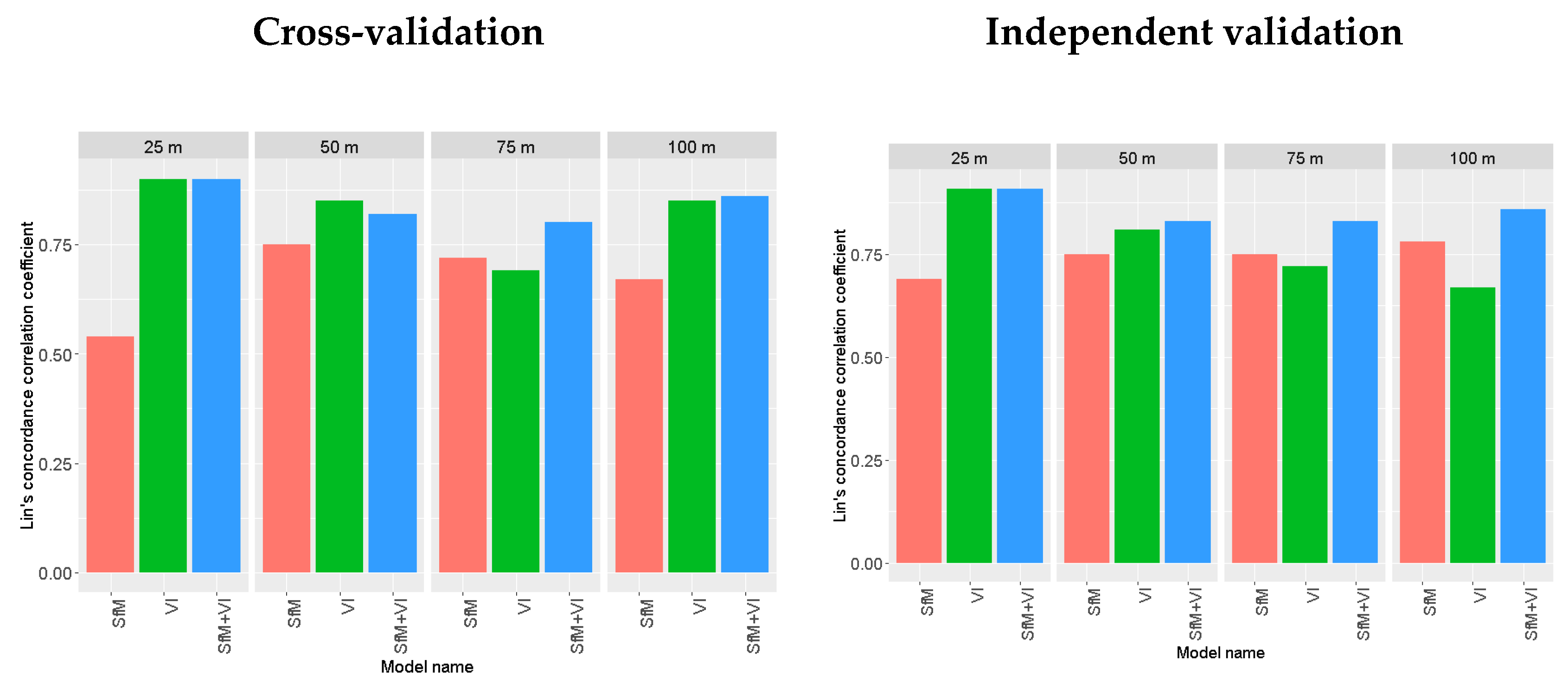
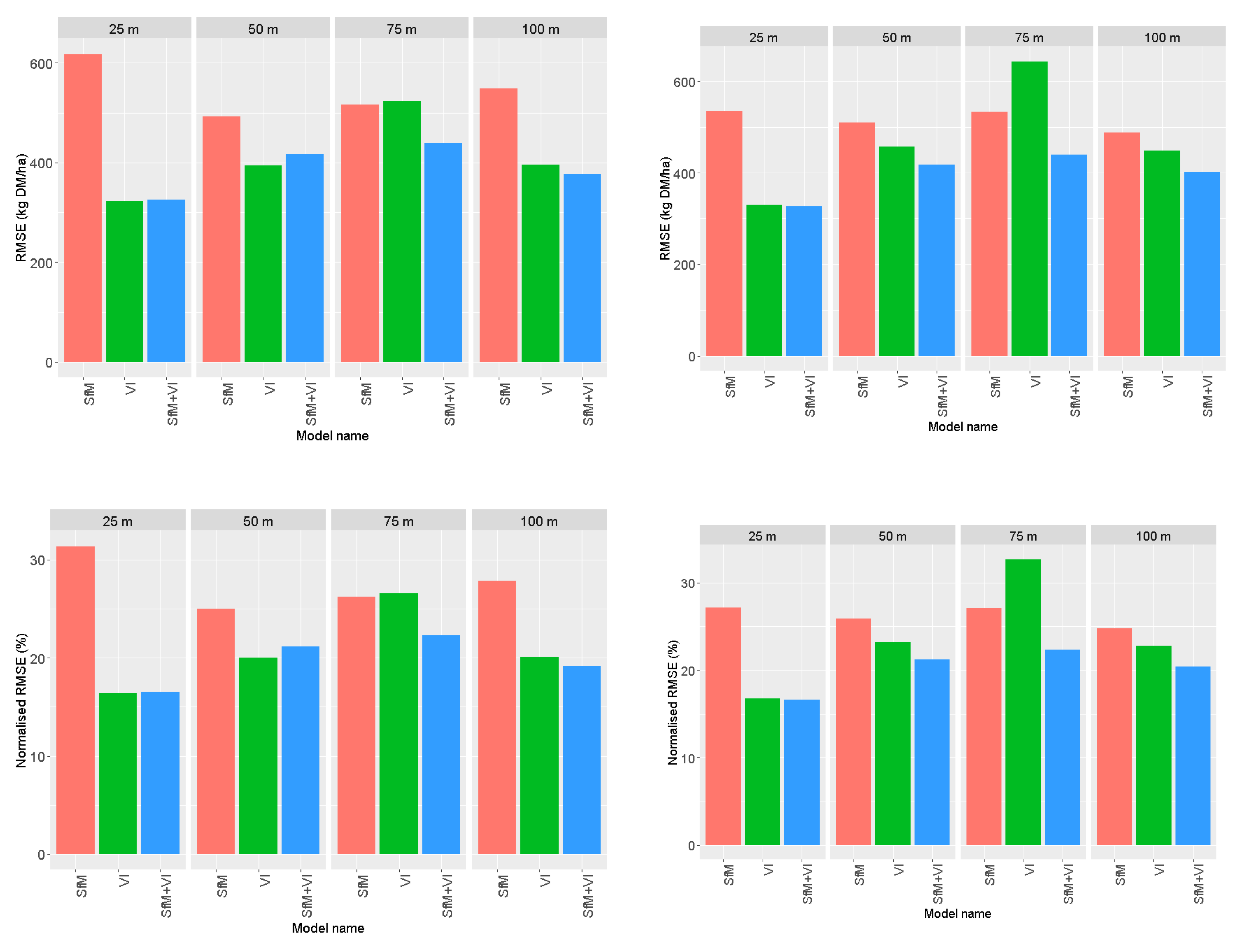
3.4. Evaluation of the Model Performances

Three different models (SfM, VI and combined features of SfM+VI) were evaluated for their ability to predict pasture DM yield at the four flying altitudes. The graphical summary of model quality evaluation (both cross-validation and independent validation) based on Lin’s concordance correlation, RMSE and normalised RMSE are summarised by flying altitude in Figure 4. The detailed summary of model quality evaluation with additional indices is provided in supplementary Material Table S1 (For cross-validation) and Table S2 (for independent validation). The selection of the most parsimonious model for each flying altitude was chosen using independent validation results according to the highest LCC value and lowest RSME value.

At lower flying altitudes (25 m and 50 m) models solely developed using the SfM features reported low model quality compared to VI only and SfM+VI combined models. At 25 m, a LCC value of 0.69 and RSME of 534 kg DM/ha was reported for the SfM model while both VI and SfM+VI models reported an LCC value >0.90 and RSME of 330 and 327 kg DM/ha, respectively (Figure 4; Supplementary Material; Table S2). A similar pattern was reported for the model developed using data generated by flying at 50 m. In contrast, at higher flying altitudes (75 and 100 m), the SfM only model reported similar model quality to the VI and SfM+VI models (Figure 4). Flying at 100 m, the SfM only model reported a RMSE value of 488 kg DM/ha, while VI and SfM+VI models reported 448 and 402 kg DM/ha, respectively (Figure 4; Supplementary Material; Table S2).

In summary, the best performing models for each flying altitude all reported LCC values greater than 0.80; RMSE less than 440 kg DM/ha, and normalised RMSE less than 23%. Out of all models tested, the SfM+VI model developed using data gathered from 25 m flying altitude was the best performing model with a LCC value of 0.91, and an RMSE of 327 kg DM/ha and a normalised RMSE of 16.6% (Figure 4; Supplementary Material; Table S2). Generally, the VI only and SfM+VI models reported similar model quality with little improvement gained by adding SfM features, flying at 75 m being the only observed exception.

As identical datasets were used for model calibration and validation at all altitudes, model comparison can be carried out both within and between the varying altitudes. In Figure 5, the distributions of the independently predicted values from all models are compared to the distribution of the measured pasture DM yield dataset. Despite the differences in model quality already reported (Figure 4 and Supplementary Material Tables S1 and S2), the distributions of the predicted datasets show a high level of agreement with that of the reference dataset and all overlap. In fact, linear mixed models analysis (results not shown) revealed that the models were not predicting differently enough to be statistically separable using standard means separation. This is because the differences in the means of the predicted values between models are naturally minor and not able to be picked up by traditional means separation techniques, but this does not mean that some models are not better at predicting than others, as shown by the validation metrics (Figure 4). The mean values of the predicted DM yield from each of the different models closely match with the reference pasture DM yield at ~2000 kg DM/ha (Figure 5). Notably, the best performing models for each flying altitude (the SfM+VI model in all cases) were able to correctly capture the variability between 1000 kg DM/ha to 3000 kg DM/ha (Figure 5). However, none of the models were able to predict the extreme values which were as low as 500 kg/DM per ha and greater than 4000 kg DM/ha in some instances (Figure 5).

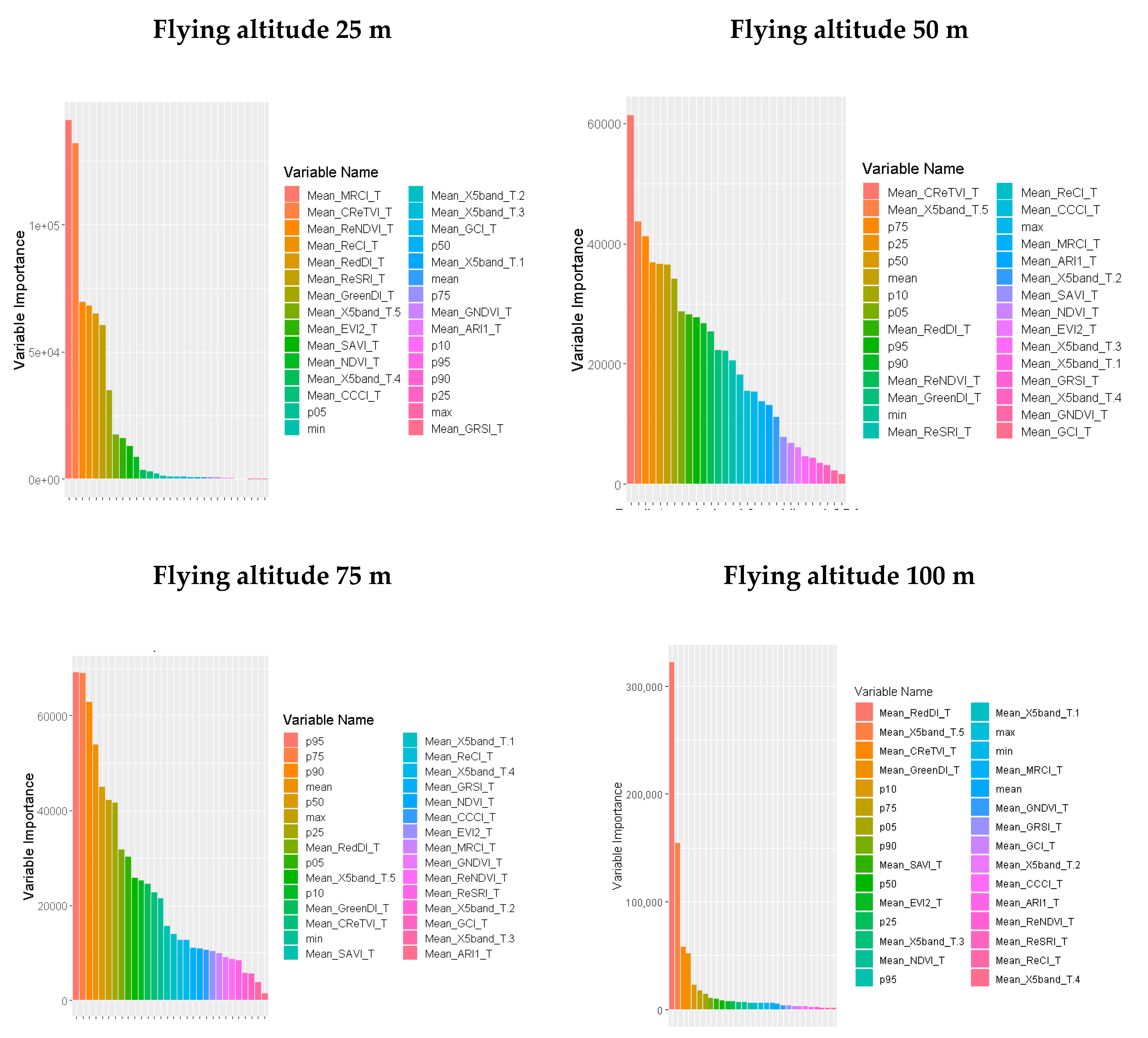
3.5. Model Drivers for Best Performing Models

The variable importance plot (VIP) associated with each fitted random forest model indicates the contribution of each feature towards the prediction of pasture DM yield. The VIP for the best performing model at each flying altitude is shown in Figure 6. Although SfM+VI models were chosen as the best performing models for all four of the flying altitudes tested, there were no SfM-derived features included within the top 10 most important features for the 25 m model (Figure 6). In contrast, the best performing models for the altitudes of 50, 75 and 100 m did rely on SfM-derived features within their top 10 most important features (Figure 6). The VIP plots for other models tested in current work (SfM only and VI only) are included in supplementary material Figure S5 (for SfM only models) and Figure S6 (for VI only models).

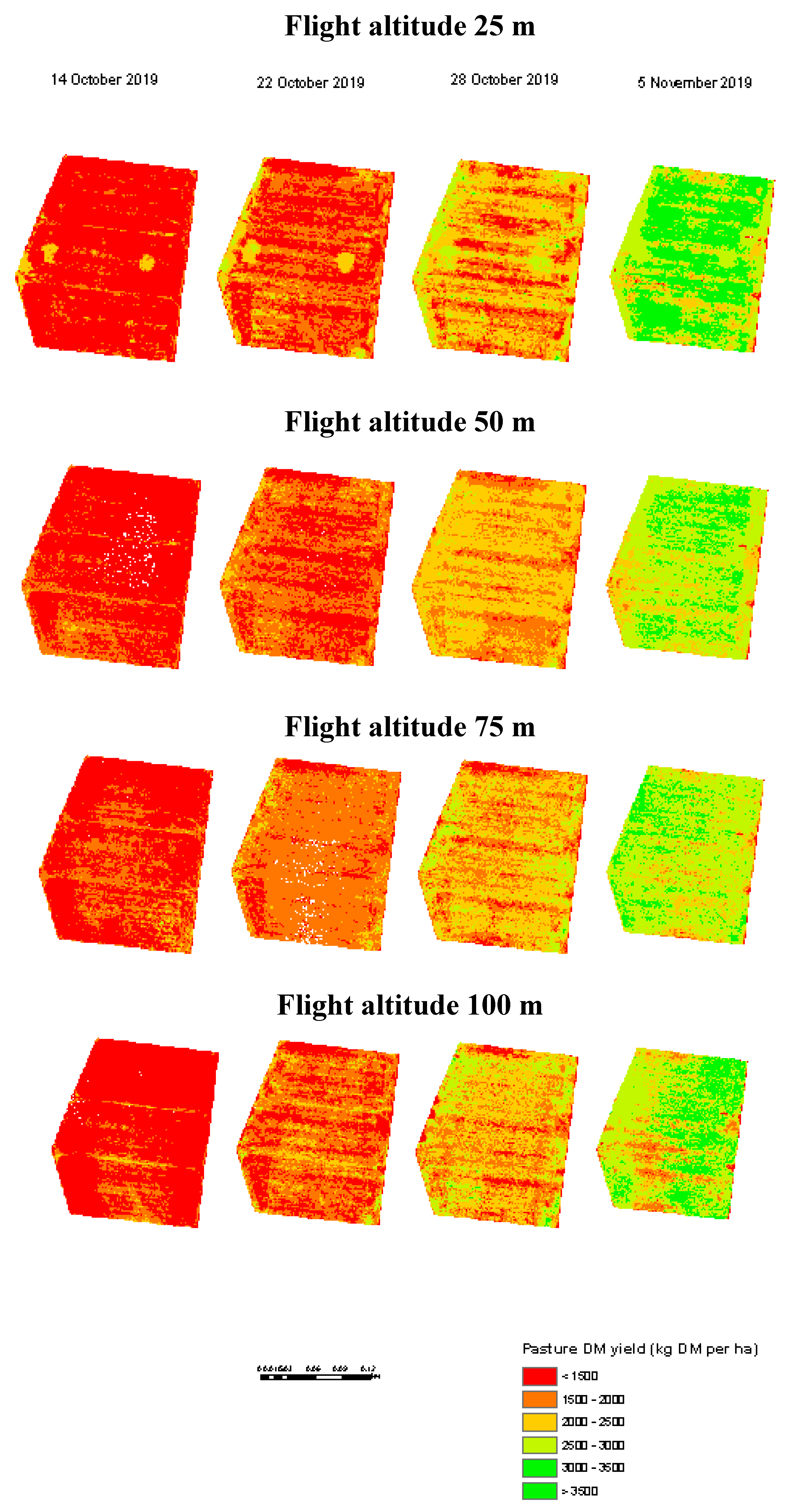
3.6. Spatial-Temporal Pasture DM Yield Maps

The best quality models were used to undertake spatial and temporal modelling of pasture DM yield across the B paddock area. Results as maps are shown in Figure 7. Although the predictions for each flying height computed, used their respective independent models, the resulting pasture DM yield predictions accounted for similar spatial estimates and patterns (Figure 7). At all altitudes, the residual pasture DM yield 2 weeks after mechanical harvesting was ~1500 kg DM/ha and by the fifth week post-cutting, was between 3000 and 3500 kg DM/ha (Figure 7).

4. Discussion

4.1. Field Data Collection, Deriving Features and Preparation of Dataset for the Model Development

Pasture DM yield is variable across the landscape and over time, and therefore requires the calculation of an appropriate number and type of features to act as explanatory model drivers. In the current study, a total of 30 features were included, that comprised 10 features derived from the CSH and associated surrogates (primarily using extracted data from Equation (2)) and 20 spectral features which included VIs, band ratios and individual reflectance bands associated with the MicaSense Rededge MX multispectral sensor (Table 4). Deriving spectral features was relatively straightforward using calibrated spectral bands and by applying known mathematical indices as outlined in Table 4. In contrast, deriving SfM-based features to act as proxies for PH was more challenging.

There are two main approaches to calculate CSH information (which, in some instances, can be referred to as 3D information in the literature) from UAV datasets. One approach is to derive both DSM and DTM in raster format. In this approach the difference between DSM and DTM is considered as the CSH and subsequent derived surrogate(s) can be included as a feature(s) in empirical model development [18]. This approach is relatively straight forward, and computation is efficient as the analysis is performed based on raster analysis. However, the use of interpolated DSMs and DTMs can result in unwanted smoothing of data. The use of such datasets at the paddock scale in the presence of heterogeneous pasture accumulation might result in lost information on the variability of CSH and its associated surrogates. In the second approach, the raw SfM point cloud dataset is used instead of an interpolated DSM raster. The difference between each point and the interpolated DTM raster of the study area is used to calculate CSH for all individual points within the point cloud [11]. However, processing and rearranging large point cloud datasets generated at the paddock scale takes additional processing time compared to the first approach and data processing methods become more complicated. In this study, a modified version of the second approach was used based on the methodology outlined by Wijesingha et al. (2019) [11].

The data quality of the CSH based approach was influenced by the accuracy of the point cloud (location and Z value) and baseline surface model (see Equation (1)) [42]. As the majority of error values were between +/−0.05 m for most of the validation panels, the estimated Z values in the point cloud data generated from the SfM algorithm can be considered as acceptable for landscape-scale analysis. It has been suggested that increasing the number of ground control points can increase the accuracy of the SfM generated datasets. In the current study, for each mission, a minimum of nine ground control points were used, noting that Wijesingha et al. (2019) [11] used only four ground control points which they considered as a minimum. Additionally, the presence of onboard L1/L2 GNSS and IMU in the UAV at the time of data capture can lead to an increase in the accuracy of the generated SfM datasets [18]. A second source of uncertainty within the CSH and its associated surrogates is introduced through the accuracy of the baseline surface model used in Equation (1). In the current study, the baseline DSM model (derived for each flying height) was initially used to estimate CSH and associated surrogates (as a proxy for height grown since cutting, not full canopy height). However, the use of baseline DSM reported missing values for individual calibration quadrats especially associated with the first and second field data collection campaigns. Furthermore, replacing the baseline DSM with baseline DTM did not improve the number of quadrats with missing data. Therefore, to overcome this problem with an aim to maximise the number of quadrat datasets for modelling, a pragmatic approach was taken to apply a constant offset of 7 cm to the baseline DSM prior to calculation using Equation (2) for each survey to bring it back in line with ground level. Similarly, Borra-Serrano et al. (2019) [43], used a correction factor of 5 cm to their baseline DTM to remove the effects of remaining stubble. It was observed that sward density was low for the first two field measurement weeks. Given mowing height a week prior to commencement of the baseline week was ~5 cm, the addition of a further 2 cm in height to compensate for pasture accumulation prior to the first measurement period seemed a reasonable approach. Work by Viljanen et al. (2018) [18] confirmed that the ability of SfM-derived features to act as proxies for canopy height in pasture production systems were limited at the initial stage of the growth periods. Moreover, it was reported that filtering steps in multi-view image processing procedures that are part of SfM algorithms could decrease data from lower vegetation canopies due to limited height variation [11,24]. This previous work has also reported similar uncertainties associated with the calculation of CSH using a baseline surface model. This was observed when a trial and error method was used to determine the optimum spatial resolution for DTM interpolation using data generated from a terrestrial laser scanner which was later included as baseline surface model aiming to minimize the “no data” records [11]. Viljanen et al. (2018) [18] generated both automatic and manual DTMs, where the latter was generated through classifying the point cloud as either ground or non-ground points. In the manual process, specifically selected ground point cloud datasets were interpolated and subsequently used to generate the optimum surface as a baseline DTM. However, they concluded that there was no difference between the generated DTMs. Similar to Viljanen et al. (2018) [18], Wijesingha et al. (2019) [11], Michez et al. (2009) [22] also used another sensor (aerial LiDAR) to generate baseline DTM. It is important to note that all these studies were undertaken on relatively small areas with flat landscapes compared to the heterogeneous landscape reported in the current paddock scale study. There are other approaches such as the use of RTK GPS to generate a higher spatial resolution DTM that can be ultimately used as baseline DTM for the generation of the CSH and associate surrogates [43]. Therefore, the use of aerial LiDAR or RTK GPS DTMs needs to be evaluated in future paddock scale studies when calculating CSH using Equation (1) and its associated surrogates.

With any study, use of the most appropriate samples for model calibration and validation is a critical step towards rigorous model development. As shown in Figure 3, there is an inherent variability in pasture DM yield across the sub-paddocks within the B paddock, and also temporal variability as samples were collected over time between post-cutting and pre-grazing. Therefore, random splitting of the dataset for model calibration and validation sets does not guarantee the inclusion of representative samples for rigorous model calibration. The use of a cLHC sampling strategy ensures that the samples that were included in model calibration represent the inherent distribution of the population datasets considering two features: (a) pixels with the sub-paddocks within the B paddock to ensure the spatial coverage and (b) measured pasture DM yield to ensure temporal variability is considered. The aim here was to capture the variability of the original dataset for pasture DM yield while simultaneously capturing the spatial representation in the calibration dataset.

Data splitting using cLHC sampling partitioned samples within the same pixel for either calibration or validation dataset. It could be hypothesised that pasture DM yield measurements within the pixel (10 × 10 m) would have had similar values in contrast to the variability between pixels. However, the generated strip chart (Figure S3) shows that there was, in fact, substantial variation of pasture DM yield within pixels, within each sub-paddock and with time. For instance, the average difference between minimum and maximum observed quadrat dry matter yield (i.e., the range) within a ‘pixel × time’ observation was 666 kg DM/ha. The median range was 604 kg DM/ha. Additionally, the calculated range as a percentage of mean dry matter reported on average was 37%. Therefore, in general pasture DM yield within a pixel could vary by half a tonne DM per hectare (T DM/ha) at any timepoint depending on location sampled. This degree of variation of pasture DM yield within a pixel is attributed to factors such as elevation, soil moisture, differential grazing intensity, differential weed loading, etc. that all affect the pasture dry matter accumulation even within a pixel at a given time step. Additionally, the sampling area of the pixel was 100 m² (10 × 10 m) and quadrat area was 0.25 m² (0.35 × 0.70 m). Therefore, the area of the quadrat to pixel area as a percentage was 0.25%, which enabled us to capture this high variability within the 10 × 10 m pixels.

4.2. Modelling Framework and Key Features Associated with Spatial-Temporal Dry Matter Yield Prediction

To the best of our knowledge, no previous studies have attempted to compare empirical models at various flying altitudes and simultaneously evaluate model drivers derived using SfM only, VI only and combined SfM+VI features using (a) a single multispectral sensor, (b) a machine learning modelling framework and (c) predictions at the scale of a commercial paddock. As a result, there are no direct studies that can be used as a comparison with the current study. However, there are a small number of studies undertaken using similar modelling frameworks, through rearrangement of features derived from SfM, VI and their combination of features in modelling pasture DM yield [11,18,22].

There are a number of frameworks that can be used for the development of models using data generated from sensors attached to UAVs to predict pasture DM yield. These frameworks can be broadly classified as (a) empirical models [11] and (b) hybrid models [4], where the latter fuses UAV datasets with simulation models. The empirical pasture prediction models can be developed using either parametric (traditional statistical) or nonparametric (machine learning) modelling approaches [44]. Generally, parametric modelling approaches are used for empirical model development to predict pasture DM yield. In most instances, either simple linear [11] or nonlinear [4] regression models were developed with the aid of commonly used VIs such as NDVI [4] or using selected SfM-derived surrogates [11]. There are studies that utilised multiple linear regression models and used different features from SfM, VI and in combinations (SfM+VI) as model drivers [22]. In this study, the development of empirical models considered a variety of features (n = 30) derived from UAV datasets using nonparametric models which consist of a machine learning algorithm. There has been an increasing trend towards the usage of machine learning algorithms over classical statistical approaches over the past few years in the development of empirical models to predict pasture DM yield and associated nutritive parameters (see, e.g., in [18,45]). This is mainly due to the advantages of machine learning models over the classical statistical approaches, especially in landscape-scale modelling because of their ability to accommodate complex relationships for either linear or nonlinear, highly correlated features, and fewer model development assumptions are required compared to the classical statistical model fitting process.

Based on the top 10 features identified through the VIP plots for the best performing model (Figure 6) it was evident that when flying at a higher altitude, the importance of the CSH surrogates derived from SfM was greater for the prediction of pasture DM yield. This may be because (a) at higher altitude there is an increase in the separation of distinctive canopy elements and (b) an increase in the field of view at higher altitudes may improve the generation of the 3D point cloud. In general, higher-order quantiles (e.g., p75) of the SfM derived surrogates were included in previous studies as model drivers [11]. By contrast, in this study, models were developed to predict pasture DM yield over time between post-cutting and pre-grazing. Therefore, in VIP plots, presence of lower-order quantiles, such as p10, p25 and p50, were identified within the top 10 important features that enables us to explain both lower and higher pasture DM yield over the time (Figure 6). In terms of spectral features, the CReTVI was identified as a top-five feature through VIP plots for flying altitude models 25 m, 50 m and 100 m, respectively (Figure 6). This index is used for estimation of high biomass in corn and shows promise as a good predictor of pasture DM yield [30]. In particular, this feature was shown to be important where higher pasture DM yields were observed. It is also important to note that, the calibrated near-infrared band and VIs derived using red-edge and near-infrared bands (see Figure 6) were also identified within the top ten features as important for pasture DM yield prediction at various flying heights (Figure 6). The use of narrow band indices is key to overcoming issues with saturation with regard to pasture DM yield estimation [46]. Furthermore, NDVI, which is the most commonly used VI for pasture DM yield modelling, was identified as less important for all flying altitudes. In fact, NDVI was not included within the top 10 features identified for the best performing model for any of the flying altitudes (Figure 6). This indicates a flaw in studies that have relied on NDVI alone for pasture DM yield prediction in the past, perhaps due to the known problems with its saturation at higher biomass.

4.3. Comparison of the Model Quality

Wijesingha et al. (2019) [11] developed a series of pasture DM yield prediction models through deriving features from SfM dataset collected at 25 m using an RGB sensor. The grassland-specific model they developed is similar to the SfM only model developed in this study using 25 m flight altitude data. In terms of model accuracy, they reported normalised RMSE value of 32.1% and 22.1% for two grassland locations (with an average value of 27.1%). The model accuracies, i.e., RMSE, were 410 kg DM/ha and 180 kg DM/ha (with an average value of 295 kg DM/ha) respectively. In comparison, the current study reported a normalised RMSE value of 27.2% using the SfM only model, which is almost equal to what has been reported by Wijeshingha et al. (2019) [11]. In terms of RMSE, the current study reported a higher value for SfM only model (534 kg DM/ha) than compared to Wijeshingha et al. (2019) [11]. However, after combining SfM+VI features in the current study, a normalised RMSE value of 16.6% was achieved, which was an improvement over that reported by Wijeshingha et al. (2019) [11] for data collected at 25 m. The best performing model for 25 m in the present study has an RMSE of 327 kg DM/ha which was nearly 100 kg DM/ha better than the average value reported for both sites by Wijeshingha et al. (2019) [11]. Notably, there are three main differences between this study and Wijeshingha et al. (2019) [11] namely; (a) the latter used grid-based data collection vs. the single grid pattern approach adopted in the current study; (b) use of an RGB sensor vs. the use of the multispectral sensor in this study; and (c) use of a simple linear regression model with the predicting feature being selected based on the highest correlation with pasture DM yield vs. use of all features with a model developed using a machine learning algorithm in the current study. Furthermore, Wijesingha et al. (2019) [11], reported that the model prediction capabilities decreased with an increase in species richness and spatial heterogeneity. In the current study, the paddock was predominantly a PRG monoculture, but the landscape was highly heterogeneous. While there is always room to improve prediction equations by increasing the size of the calibration dataset, the initial results presented here can be considered acceptable for paddock scale estimation of pasture DM yield.

Viljanen et al. (2018) [18] developed a series of empirical models through a combination of SfM data (they referred to as 3D), RGB data and VI datasets very similar to the current study. In their case, they collated RGB datasets at 30 m and hyperspectral data at 50 m (the latter sensor was only used to gather NIR and Red spectral information for calculation of VIs). They fused all the derived features and utilised a Random Forest modelling framework to develop empirical models like the current study. They reported an RMSE of 400 kg DM/ha and a normalised RMSE value of 15.1%. These results were obtained through LOOCV results as opposed to the independent validation which was adopted in the present study for robust evaluation of model performances. In the present study at 25 m and 50 m, the best performing models had an RMSE of 327 kg DM/ha and 418 kg DM/ha and normalised RMSE values of 16.6% and 21.2%. As such, the 25 m model from this study can be considered slightly better than the model reported by Viljanen et al. (2018) [18]. The notable differences between these two studies include; (a) sensor datasets generated at two different flying altitudes, which were then fused in model development compared to the current study where both SfM and spectral feature datasets were independently derived at all flying altitudes using a single multispectral sensor; (b) postprocessing of images using onboard RTK GPS data to obtain an accurate correction of locations, which was not possible in the current study. On a practical note, having just one sensor onboard the UAV reduces the draw on battery life and enables the ability to produce similar validation statistics for inter-model comparison.

Michez et al. (2019) [22] also developed pasture DM yield models using 3D, spectral and a combination of 3D and spectral data, similar to the current study. Like this study, they also concluded that the fused model was the best performing of those tested. Their models were validated using a k-fold validation approach, and the most parsimonious model was fitted through the variable selection and by fitting multiple linear models. Furthermore, they reported an adjusted R² value of 0.49 and RMSE value 900 kg DM/ha (originally reported as 0.09 kg/m²). In contrast, the best performing machine learning model generated in the current study flying at the same altitude (50 m) reported an R² value of 0.79 and RMSE value of 418 kg DM/ha for independent validation. Notably, and similar to Viljanen et al. (2018) [18], work undertaken by Michez et al. (2019) [22], also used two sensors to collect RGB and multispectral data where the first sensor was used for generation of DSM and later used for the generation of a series of VIs. In both the current study and Viljanen et al. (2018) [18], derived surrogates from SfM data were included in modelling while Mitchez et al. (2019) [22] simply used the difference between ‘DSM-DTM’ and included CSH as a feature in the model development.

The model generated at 25 m outperformed the other flying altitude models; however, in practical terms, generating UAV data at 100 m has a lot of advantages for farm scale applications: (a) more coverage of land extent, (b) shorter time for UAV data acquisition and (c) smaller file sizes which enables fast pre/postprocessing of collected datasets. In fact, the RMSE difference between the 25 m and 100 m flying altitude models was only 75 kg DM/ha (402 kg DM/ha − 327 kg DM/ha) in terms of model accuracy. Therefore, on a practical note, collection of UAV data at 100 m flying altitude is more suitable for farm scale applications. Additionally, models developed in the current study can be updated when the new datasets are available which will improve the ability to characterise inherent variability of the pasture DM yield.

4.4. Practical Uses of the Derived Maps

While the maps produced from this study provide detailed information on the spatial distribution of pasture DM yield with time these derived spatial datasets can be utilised to create paddock scale management zones. Paddock management zones are frequently applied across broadacre cropping systems but are not generally used in dairy systems for on-farm management decision making such as grazing and feed budget calculations that consider each individual paddock. With the availability of technologies such as virtual fencing, the creation of management zones within a given paddock may improve allocation of both pasture “quantity” and “quality” when considering herd requirements and pasture renovation [22].

4.5. Limitations and Uncertainties Associated with the Current Study, Recommendations and Future Directions

One of the major uncertainties of this study is associated with deriving CSH and associated surrogates using SfM datasets as described under Section 4.1. While generated SfM data reported reasonable accuracy, much attention needs to be given to generating a good quality baseline surface model as outlined above. Additionally, in-field data acquisition with a combination of oblique and nadir drone angles is reported to increase the quality of the SfM data [18]. It has also been reported that wind during flights affects the quality of the SfM datasets [47]. On a practical note, such issues are difficult to overcome in landscape-scale analysis such as those in the current study.

The model developed in the current study is specifically targeted for the spring growth season and there were a limited number (n = 20) of independent samples for model validation. Additional datasets are required to test the model’s ability to predict pasture DM yield in other seasons. Such datasets could be used to update the current model if necessary. Additionally, ancillary features such as weather, soil and topography could be incorporated into the future modelling framework. A study carried out by Borra-Serrano et al. (2019) [43] included rearranged weather data as growing degree days, days since last defoliation (difference between cut date and measurement date), and SfM with spectral data for empirical model drivers to predict pasture DM yield. It is anticipated that the fusion of different spatial and temporal support datasets will play a major role in empirical model development targeting pasture DM yield in space-time in the near future.

Having correlated features as model drivers is less of an issue for tree model predictions that are developed as ensemble models, especially when feature bagging is employed such as in the Random Forest modelling approach. However, having correlated features can influence the estimation of individual feature importance in the VIPs. In ensemble modelling frameworks, there are different approaches to carry out feature selection to remove correlated or less important features. For example, Gregorutti et al. (2016) [48] used the recursive feature elimination algorithm for variable selection using a permutation importance measure as a ranking criterion. Additionally, to ensure the stability in variable selection, the Boruta feature selection algorithm can be coupled with the random forest modelling approach [49]. As no feature selection was carried out in the current study, it can be considered as limitation of this study.

5. Conclusions

This study revealed the potential of using aerial multispectral datasets for the spatial-temporal prediction of pasture DM yield at a paddock scale. In terms of model performances, models developed using all four tested flying altitudes revealed that the combination of SfM+VI model outperformed SfM only and VI only models, particularly at high altitudes. The study also highlighted the limitations associated with deriving features from SfM datasets especially with the baseline surface model. In terms of model quality, data generated at 25 m flying altitude reported the best performing model although differences between all model performances were minor. For practical applications on real farms, use of data generated at higher altitudes, i.e., 100 m can produce models that are nearly as accurate as 25 m models but with greatly reduced complexity of data collection.

References

1. Garcia, S.C.; Clark, C.; Kerrisk, K.; Islam, M.; Farina, S.; Evans, J. Gaps and Variability in Pasture Utilisation in Australian Pasture-Based Dairy Systems. In Proceedings of the 22nd International Grasslands Congress, Sydney, Australia, 15–19 September 2013. [Google Scholar]
2. Wales, W.J.; Kolver, E.S. Challenges of Feeding Dairy Cows in Australia and New Zealand. Anim. Prod. Sci. 2017, 57, 1366–1383. [Google Scholar] [CrossRef] [Green Version]
3. Jacobs, J.L. Challenges in Ration Formulation in Pasture-Based Milk Production Systems. Anim. Prod. Sci. 2014, 54, 1130–1140. [Google Scholar] [CrossRef]
4. Insua, J.R.; Utsumi, S.A.; Basso, B. Estimation of Spatial and Temporal Variability of Pasture Growth and Digestibility in Grazing Rotations Coupling Unmanned Aerial Vehicle (UAV) with Crop Simulation Models. PLoS ONE 2019, 14, e0212773. [Google Scholar] [CrossRef] [PubMed] [Green Version]
5. Santillan, R.A.; Ocumpaugh, W.R.; Mott, G.O. Estimating Forage Yield with a Disk Meter1. Agron. J. 1979, 71, 71–74. [Google Scholar] [CrossRef]
6. Earle, D.; McGowan, A. Evaluation and Calibration of an Automated Rising Plate Meter for Estimating Dry Matter Yield of Pasture. Aust. J. Exp. Agric. 1979, 19, 337–343. [Google Scholar] [CrossRef]
7. Sanderson, M.A.; Rotz, C.A.; Fultz, S.W.; Rayburn, E.B. Estimating Forage Mass with a Commercial Capacitance Meter, Rising Plate Meter, and Pasture Ruler. Agron. J. 2001, 93, 1281–1286. [Google Scholar] [CrossRef] [Green Version]
8. Legg, M.; Bradley, S. Ultrasonic Proximal Sensing of Pasture Biomass. Remote Sens. 2019, 11, 2459. [Google Scholar] [CrossRef] [Green Version]
9. Trotter, M.G.; Lamb, D.W.; Donald, G.E.; Schneider, D.A. Evaluating an Active Optical Sensor for Quantifying and Mapping Green Herbage Mass and Growth in a Perennial Grass Pasture. Crop Pasture Sci. 2010, 61, 389–398. [Google Scholar] [CrossRef]
10. Schaefer, T.M.; Lamb, W.D. A Combination of Plant NDVI and LiDAR Measurements Improve the Estimation of Pasture Biomass in Tall Fescue (Festuca Arundinacea Var. Fletcher). Remote Sens. 2016, 8, 109. [Google Scholar] [CrossRef] [Green Version]
11. Wijesingha, J.; Moeckel, T.; Hensgen, F.; Wachendorf, M. Evaluation of 3D Point Cloud-Based Models for the Prediction of Grassland Biomass. Int. J. Appl. Earth Obs. Geoinf. 2019, 78, 352–359. [Google Scholar] [CrossRef]
12. Grüner, E.; Astor, T.; Wachendorf, M. Biomass Prediction of Heterogeneous Temperate Grasslands Using an SfM Approach Based on UAV Imaging. Agronomy 2019, 9, 54. [Google Scholar] [CrossRef] [Green Version]
13. Edirisinghe, A.; Hill, M.J.; Donald, G.E.; Hyder, M. Quantitative Mapping of Pasture Biomass Using Satellite Imagery. Int. J. Remote Sens. 2011, 32, 2699–2724. [Google Scholar] [CrossRef]
14. Edirisinghe, A.; Clark, D.; Waugh, D. Spatio-Temporal Modelling of Biomass of Intensively Grazed Perennial Dairy Pastures Using Multispectral Remote Sensing. Int. J. Appl. Earth Obs. Geoinf. 2012, 16, 5–16. [Google Scholar] [CrossRef]
15. Bendig, J.; Bolten, A.; Bennertz, S.; Broscheit, J.; Eichfuss, S.; Bareth, G. Estimating Biomass of Barley Using Crop Surface Models (CSMs) Derived from UAV-Based RGB Imaging. Remote Sens. 2014, 6, 10395–10412. [Google Scholar] [CrossRef] [Green Version]
16. Han, L.; Yang, G.; Dai, H.; Xu, B.; Yang, H.; Feng, H.; Li, Z.; Yang, X. Modeling Maize Above-Ground Biomass Based on Machine Learning Approaches Using UAV Remote-Sensing Data. Plant Methods 2019, 15, 10. [Google Scholar] [CrossRef] [PubMed] [Green Version]
17. Bendig, J.; Yu, K.; Aasen, H.; Bolten, A.; Bennertz, S.; Broscheit, J.; Gnyp, M.L.; Bareth, G. Combining UAV-Based Plant Height from Crop Surface Models, Visible, and near Infrared Vegetation Indices for Biomass Monitoring in Barley. Int. J. Appl. Earth Obs. Geoinf. 2015, 39, 79–87. [Google Scholar] [CrossRef]
18. Viljanen, N.; Honkavaara, E.; Näsi, R.; Hakala, T.; Niemeläinen, O.; Kaivosoja, J. A Novel Machine Learning Method for Estimating Biomass of Grass Swards Using a Photogrammetric Canopy Height Model, Images and Vegetation Indices Captured by a Drone. Agriculture 2018, 8, 70. [Google Scholar] [CrossRef] [Green Version]
19. Lussem, U.; Bolten, A.; Gnyp, M.L.; Jasper, J.; Bareth, G. Evaluation of RGB-Based Vegetation Indices from UAV Imagery to Estimate Forage Yield in Grassland. ISPRS Int. Arch. Photogramm. Remote Sens. Spat. Inf. Sci. 2018, 42, 1215–1219. [Google Scholar] [CrossRef] [Green Version]
20. Gebremedhin, A.; Badenhorst, P.; Wang, J.; Giri, K.; Spangenberg, G.; Smith, K. Development and Validation of a Model to Combine NDVI and Plant Height for High-Throughput Phenotyping of Herbage Yield in a Perennial Ryegrass Breeding Program. Remote Sens. 2019, 11, 2494. [Google Scholar] [CrossRef] [Green Version]
21. Geipel, J.; Korsaeth, A. Hyperspectral Aerial Imaging for Grassland Yield Estimation. Adv. Anim. Biosci. 2017, 8, 770–775. [Google Scholar] [CrossRef]
22. Michez, A.; Lejeune, P.; Bauwens, S.; Herinaina, A.A.; Blaise, Y.; Castro Muñoz, E.; Lebeau, F.; Bindelle, J. Mapping and Monitoring of Biomass and Grazing in Pasture with an Unmanned Aerial System. Remote Sens. 2019, 11, 473. [Google Scholar] [CrossRef] [Green Version]
23. Cooper, D.S.; Roy, P.D.; Schaaf, B.C.; Paynter, I. Examination of the Potential of Terrestrial Laser Scanning and Structure-from-Motion Photogrammetry for Rapid Nondestructive Field Measurement of Grass Biomass. Remote Sens. 2017, 9, 531. [Google Scholar] [CrossRef] [Green Version]
24. Wallace, L.; Hillman, S.; Reinke, K.; Hally, B. Non-Destructive Estimation of above-Ground Surface and near-Surface Biomass Using 3D Terrestrial Remote Sensing Techniques. Methods Ecol. Evol. 2017, 8, 1607–1616. [Google Scholar] [CrossRef] [Green Version]
25. Rouse, J.; Haas, R.; Schell, J.; Deering, D. Monitoring Vegetation Systems in the Great Plains with ERTS. In Third ERTS Symposium; NASA: College Station, TX, USA, 1973; pp. 309–317. [Google Scholar]
26. Gitelson, A.A.; Kaufman, Y.J.; Merzlyak, M.N. Use of a Green Channel in Remote Sensing of Global Vegetation from EOS-MODIS. Remote Sens. Environ. 1996, 58, 289–298. [Google Scholar] [CrossRef]
27. Gitelson, A.; Merzlyak, M.N. Spectral Reflectance Changes Associated with Autumn Senescence of Aesculus hippocastanum L. and Acer platanoides L. Leaves. Spectral Features and Relation to Chlorophyll Estimation. J. Plant Physiol. 1994, 143, 286–292. [Google Scholar] [CrossRef]
28. Gitelson, A.A.; Viña, A.; Ciganda, V.; Rundquist, D.C.; Arkebauer, T.J. Remote Estimation of Canopy Chlorophyll Content in Crops. Geophys. Res. Lett. 2005, 32. [Google Scholar] [CrossRef] [Green Version]
29. Huete, A.; Didan, K.; Miura, T.; Rodriguez, E.P.; Gao, X.; Ferreira, L.G. Overview of the Radiometric and Biophysical Performance of the MODIS Vegetation Indices. Remote Sens. Environ. 2002, 83, 195–213. [Google Scholar] [CrossRef]
30. Dash, J.; Curran, P.J. The MERIS Terrestrial Chlorophyll Index. Int. J. Remote Sens. 2004, 25, 5403–5413. [Google Scholar] [CrossRef]
31. Chen, P.-F.; Tremblay, N.; Wang, J.-H.; Vigneault, P.; Huang, W.-J.; Li, B.-G. New Index for Crop Canopy Fresh Biomass Estimation. Spectrosc. Spectr. Anal. 2010, 30, 512–517. [Google Scholar] [CrossRef]
32. Tucker, C.J. Red and Photographic Infrared Linear Combinations for Monitoring Vegetation. Remote Sens. Environ. 1979, 8, 127–150. [Google Scholar] [CrossRef] [Green Version]
33. Jago, R.A.; Cutler, M.E.J.; Curran, P.J. Estimating Canopy Chlorophyll Concentration from Field and Airborne Spectra. Remote Sens. Environ. 1999, 68, 217–224. [Google Scholar] [CrossRef]
34. Sripada, R. Determining In-Season Nitrogen Requirements for Corn Using Aerial Color-Infrared Photography. Ph.D. Dissertation, North Carolina State University, Raleigh, NC, USA, 2005. [Google Scholar]
35. Sripada, R.P.; Heiniger, R.W.; White, J.G.; Meijer, A.D. Aerial Color Infrared Photography for Determining Early In-Season Nitrogen Requirements in Corn. Agron. J. 2006, 98, 968–977. [Google Scholar] [CrossRef]
36. Huete, A.R. A Soil-Adjusted Vegetation Index (SAVI). Remote Sens. Environ. 1988, 25, 295–309. [Google Scholar] [CrossRef]
37. Gitelson, A.A.; Merzlyak, M.N.; Chivkunova, O.B. Optical Properties and Nondestructive Estimation of Anthocyanin Content in Plant Leaves. Photochem. Photobiol. 2001, 74, 38–45. [Google Scholar] [CrossRef]
38. Breiman, L. Random Forests. Mach. Learn. 2001, 45, 5–32. [Google Scholar] [CrossRef] [Green Version]
39. Wright, M.N.; Ziegler, A. Ranger: A Fast Implementation of Random Forests for High Dimensional Data in C++ and R. arXiv 2015, arXiv:1508.04409. [Google Scholar] [CrossRef] [Green Version]
40. Minasny, B.; McBratney, A.B. A Conditioned Latin Hypercube Method for Sampling in the Presence of Ancillary Information. Comput. Geosci. 2006, 32, 1378–1388. [Google Scholar] [CrossRef]
41. Lawrence, I.; Lin, K. A Concordance Correlation Coefficient to Evaluate Reproducibility. Biometrics 1989, 45, 255–268. [Google Scholar] [CrossRef]
42. Shi, Y.; Thomasson, J.A.; Murray, S.C.; Pugh, N.A.; Rooney, W.L.; Shafian, S.; Rajan, N.; Rouze, G.; Morgan, C.L.; Neely, H.L.; et al. Unmanned Aerial Vehicles for High-Throughput Phenotyping and Agronomic Research. PLoS ONE 2016, 11, e0159781. [Google Scholar] [CrossRef] [Green Version]
43. Borra-Serrano, I.; De Swaef, T.; Muylle, H.; Nuyttens, D.; Vangeyte, J.; Mertens, K.; Saeys, W.; Somers, B.; Roldán-Ruiz, I.; Lootens, P. Canopy Height Measurements and Non-Destructive Biomass Estimation of Lolium Perenne Swards Using UAV Imagery. Grass Forage Sci. 2019, 74, 356–369. [Google Scholar] [CrossRef]
44. Caicedo, J.P.R. Optimized and Automated Estimation of Vegetation Properties: Opportunities for Sentinel-2; Universitat De València: Valencia, Spain, 2014. [Google Scholar]
45. Wijesingha, J.; Astor, T.; Schulze-Brüninghoff, D.; Wengert, M.; Wachendorf, M. Predicting Forage Quality of Grasslands Using UAV-Borne Imaging Spectroscopy. Remote Sens. 2020, 12, 126. [Google Scholar] [CrossRef] [Green Version]
46. Mutanga, O.; Skidmore, A.K. Narrow Band Vegetation Indices Overcome the Saturation Problem in Biomass Estimation. Int. J. Remote Sens. 2004, 25, 3999–4014. [Google Scholar] [CrossRef]
47. van Iersel, W.; Straatsma, M.; Addink, E.; Middelkoop, H. Monitoring Height and Greenness of Non-Woody Floodplain Vegetation with UAV Time Series. ISPRS J. Photogramm. Remote Sens. 2018, 141, 112–123. [Google Scholar] [CrossRef]
48. Gregorutti, B.; Michel, B.; Saint-Pierre, P. Correlation and Variable Importance in Random Forests. Stat. Comput. 2017, 27, 659–678. [Google Scholar] [CrossRef] [Green Version]
49. Kursa, M.B.; Rudnicki, W.R. Feature Selection with the Boruta Package. J. Stat. Softw. 2010, 1. [Google Scholar] [CrossRef] [Green Version]
Figure 1. Location of B paddocks (Yellow boundary) and associated 10 × 10 m sampling areas (purple squares) that were used to select three sub-samples for destructive sampling (Image source: ESRI, World Imagery).
Remotesensing 12 02017 g001
Figure 2. Data analysis approach for spatial-temporal estimation of pasture dry matter yield.
Remotesensing 12 02017 g002
Figure 3. Boxplots depicting the distribution of pasture DM yield across three sub-paddocks within the B paddocks at each of four field sampling dates. The horizontal bold black line within the boxplot depicts the mean value associated with that sub-paddock and sampling date.
Remotesensing 12 02017 g003
Figure 4. The graphical summary of the model quality evaluation using Lin’s concordance correlation, RMSE and normalised RMSE for three tested models with respect to four flying altitudes. Results are summarised for both leave-one-out cross-validation and independent validation.
Remotesensing 12 02017 g004aRemotesensing 12 02017 g004b
Figure 5. Evaluation of different model prediction capabilities with respect to the reference pasture dry matter yield in an independent validation test. All models were validated using the same independent samples (n = 20) for meaningful comparison. The horizontal black line within the boxplot depicts the estimated mean value in each case.
Remotesensing 12 02017 g005
Figure 6. The variable importance plot generated from the best performing Random Forest model developed from the data generated at different flying altitudes (Note: Refer Table 4 for abbreviations).
Remotesensing 12 02017 g006
Figure 7. The spatial-temporal prediction of pasture dry matter (DM) yield (kg DM/ha) and changes of herbage DM accumulation in measurement weeks 1–4 after mechanical harvesting, using the best performing model (SfM+VI) for flying altitude 25, 50, 75 and 100 m. Note: 14 October 2019: Measurement week 1; 22 October 2019: Measurement week 2; 28 October 2019: Measurement week 3; 5 November 2019: Measurement week 4.
Remotesensing 12 02017 g007