Validation of Carbon Trace Gas Profile Retrievals from the NOAA-Unique Combined Atmospheric Processing System for the Cross-Track Infrared Sounder

 , , ,
, , ,  , , , ,
  , , , , , , , ,
Abstract
:
1. Introduction
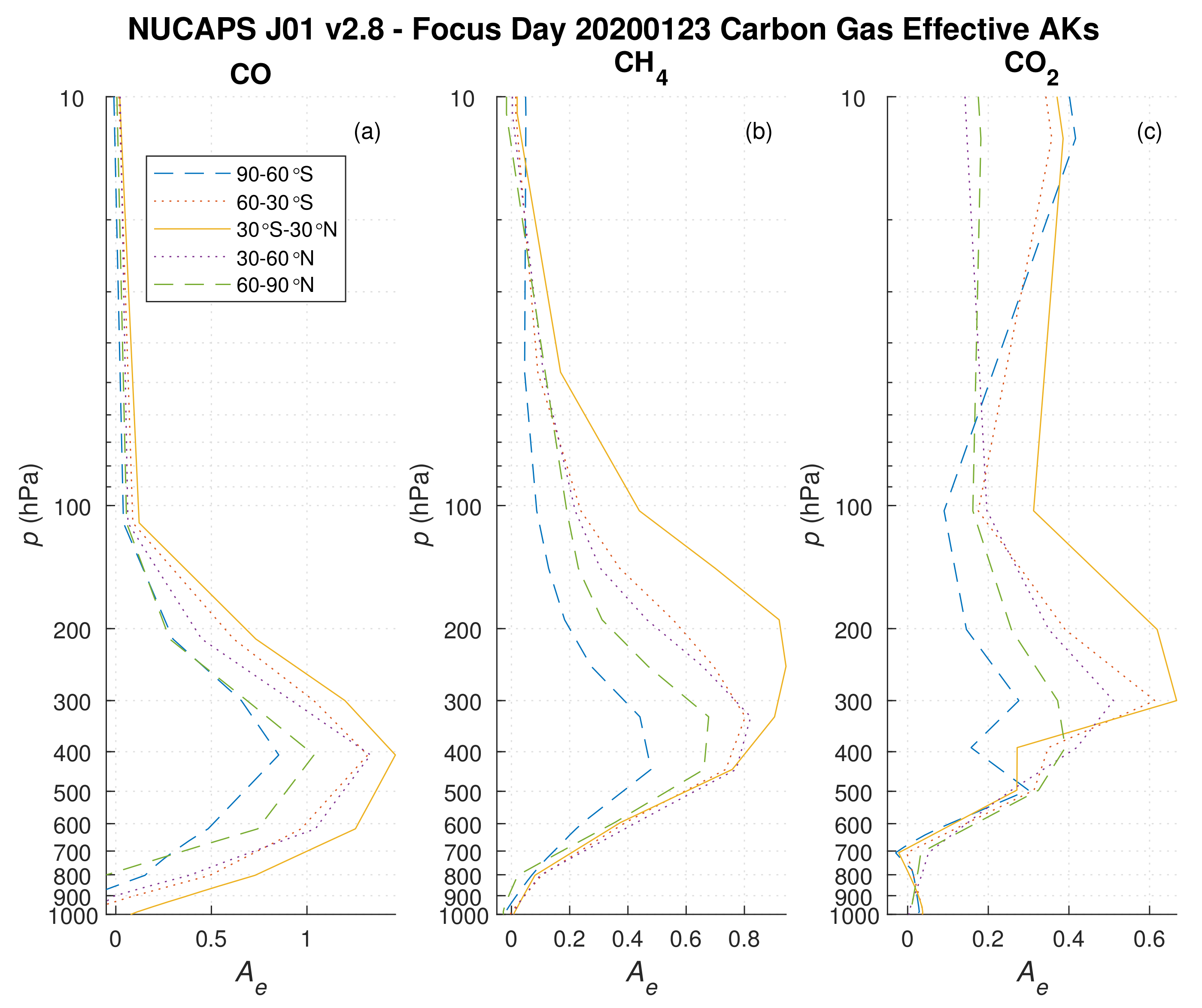
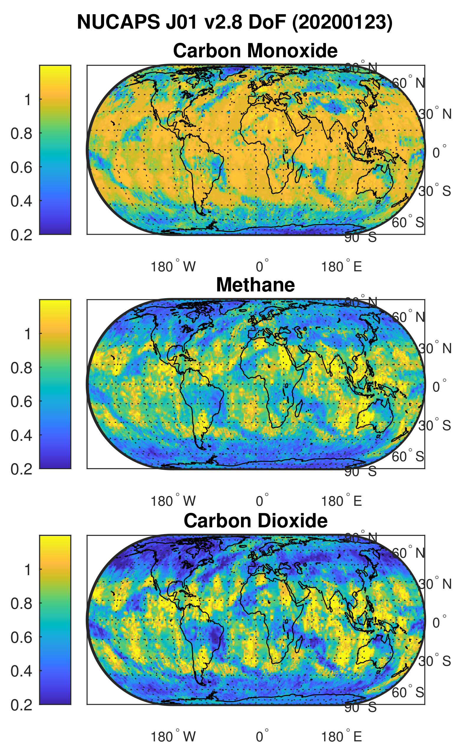
2. Methodology
3. Data
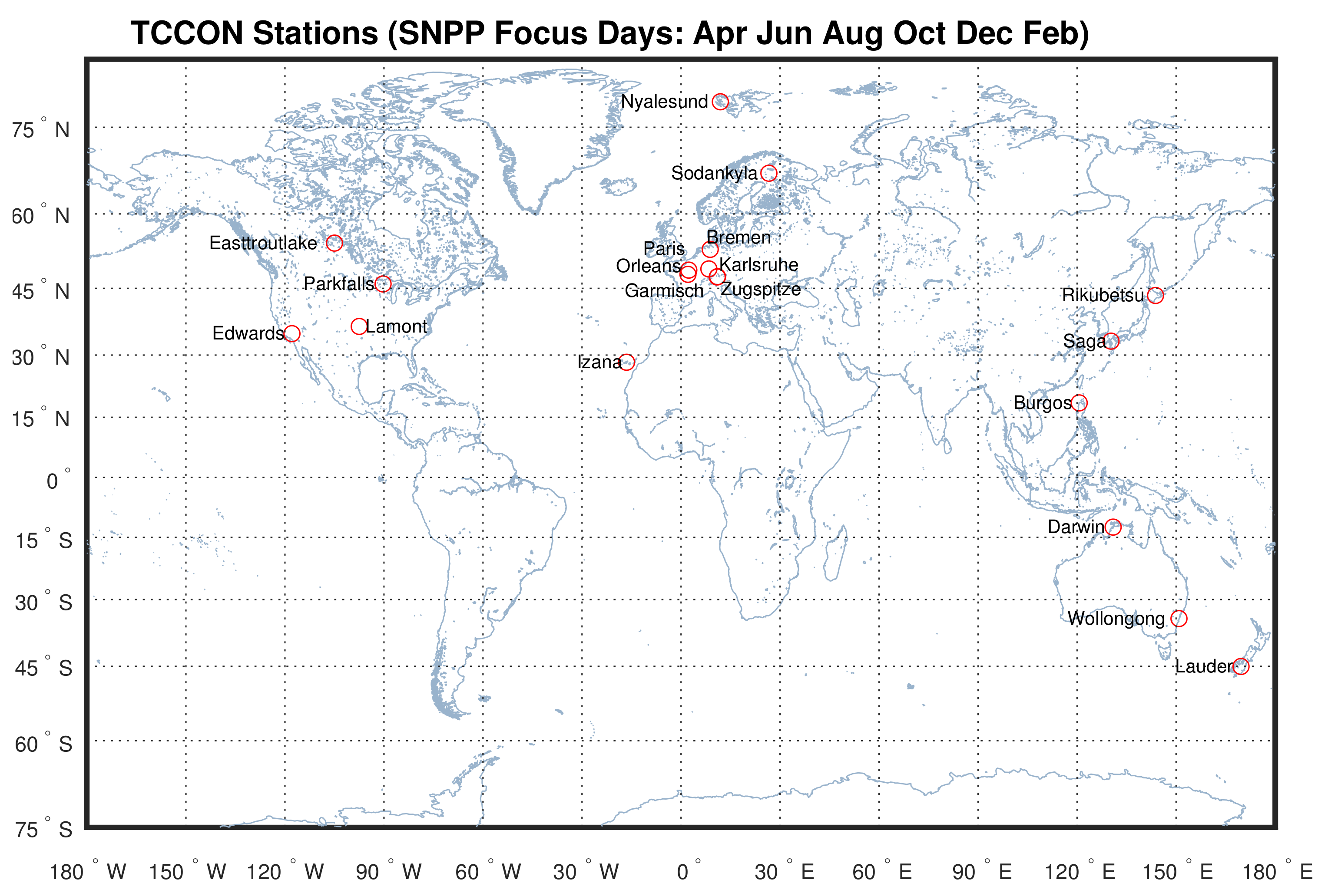
3.1. TCCON
3.2. AirCore
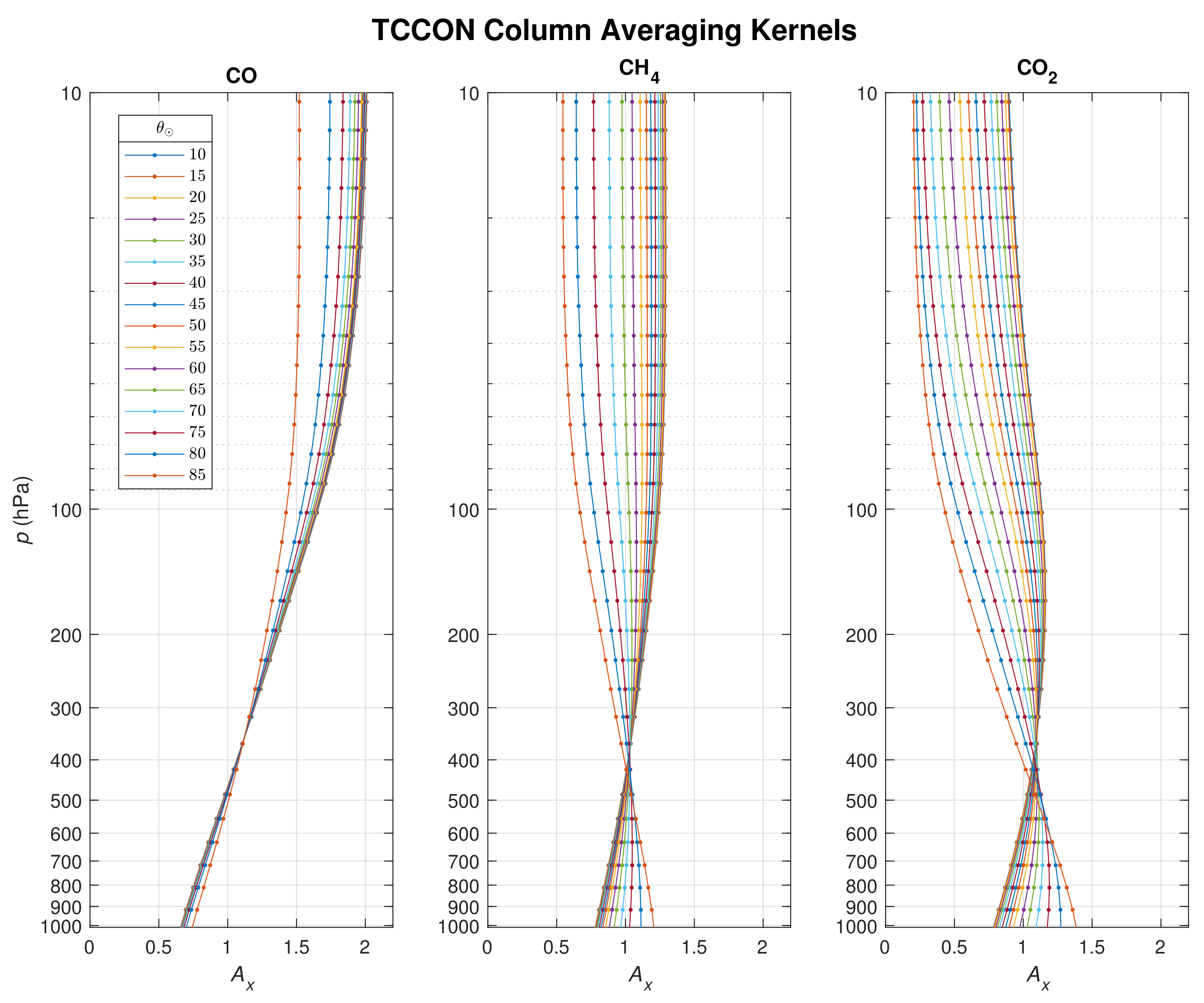
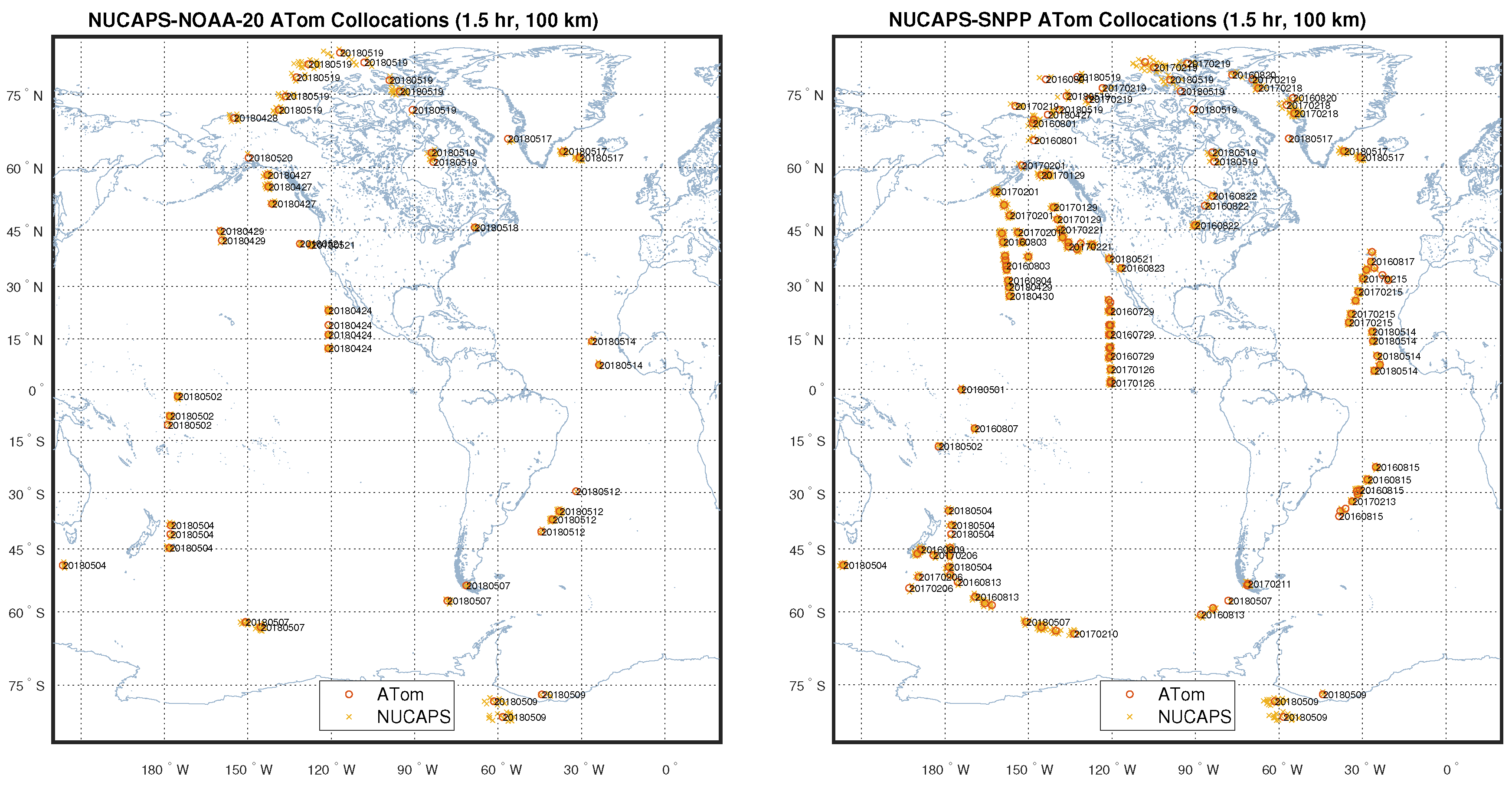
3.3. ATom
3.4. NUCAPS Retrievals
4. Results and Discussion
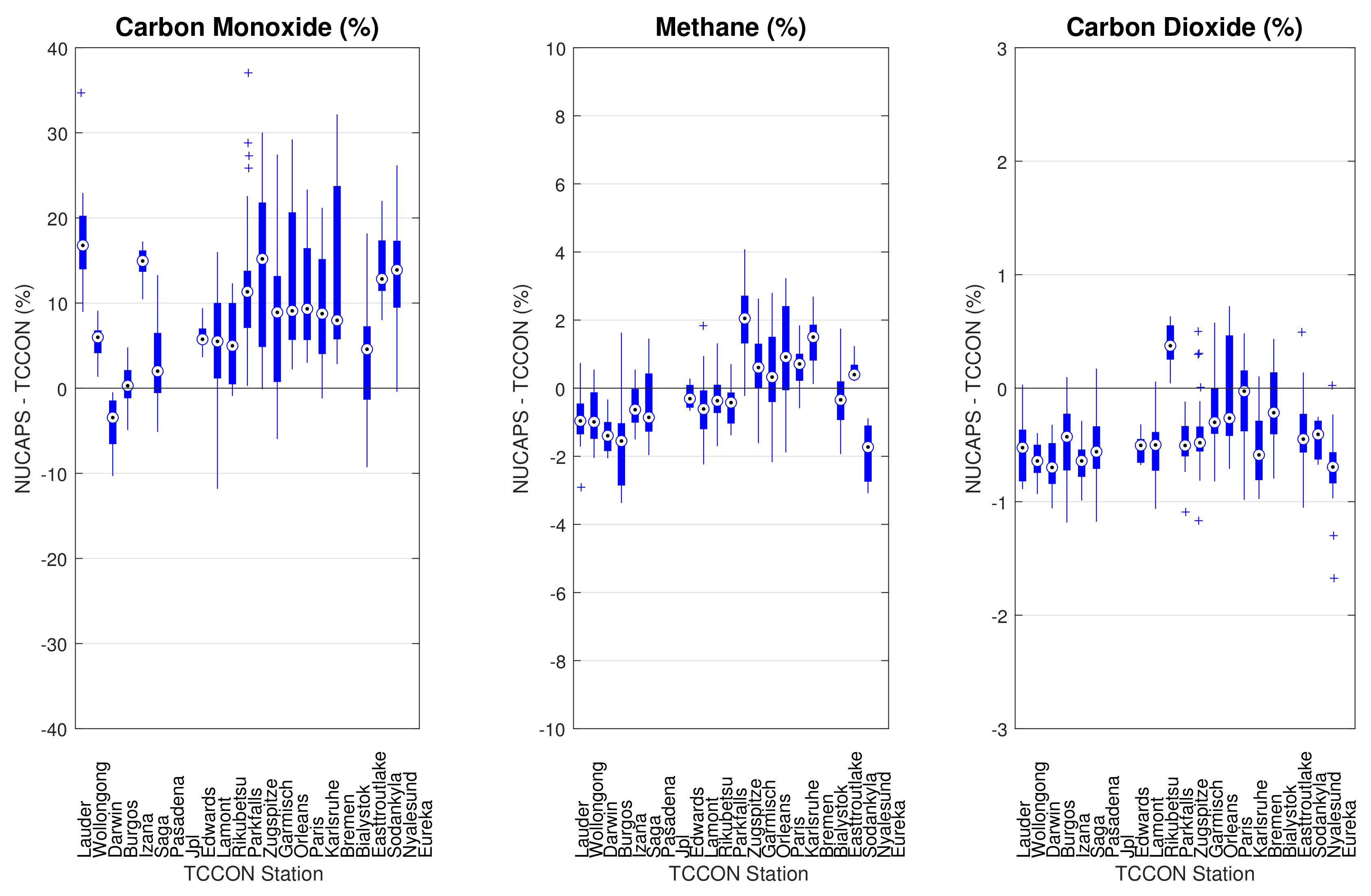
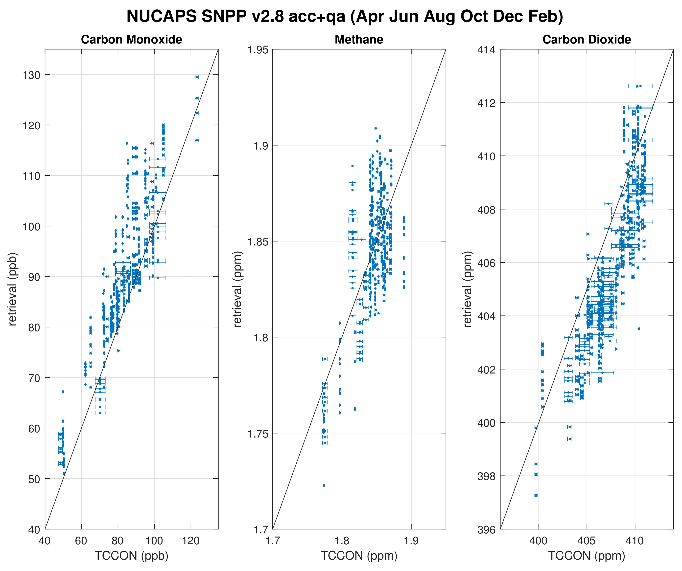
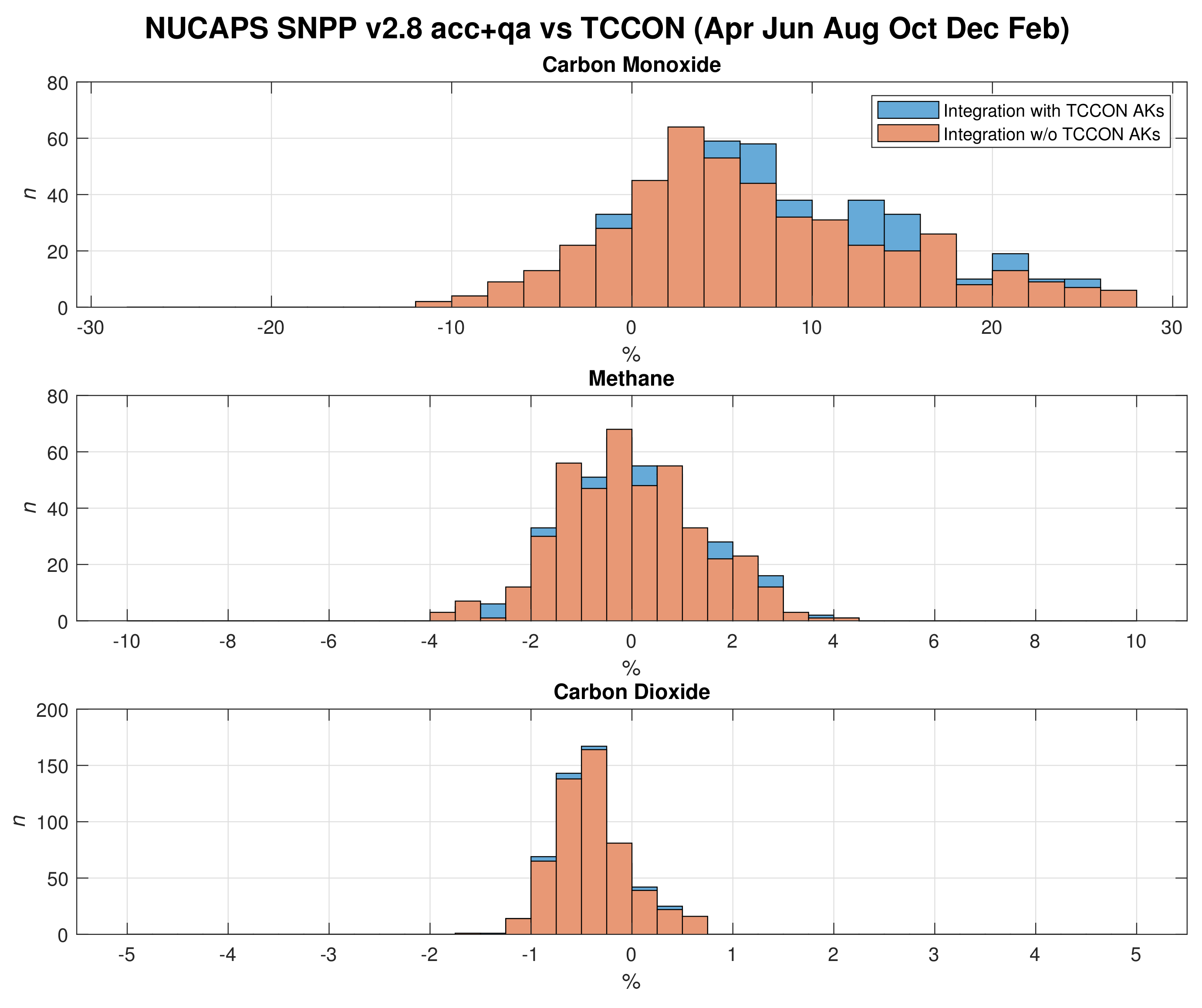
4.1. Statistical Analysis versus TCCON Baseline
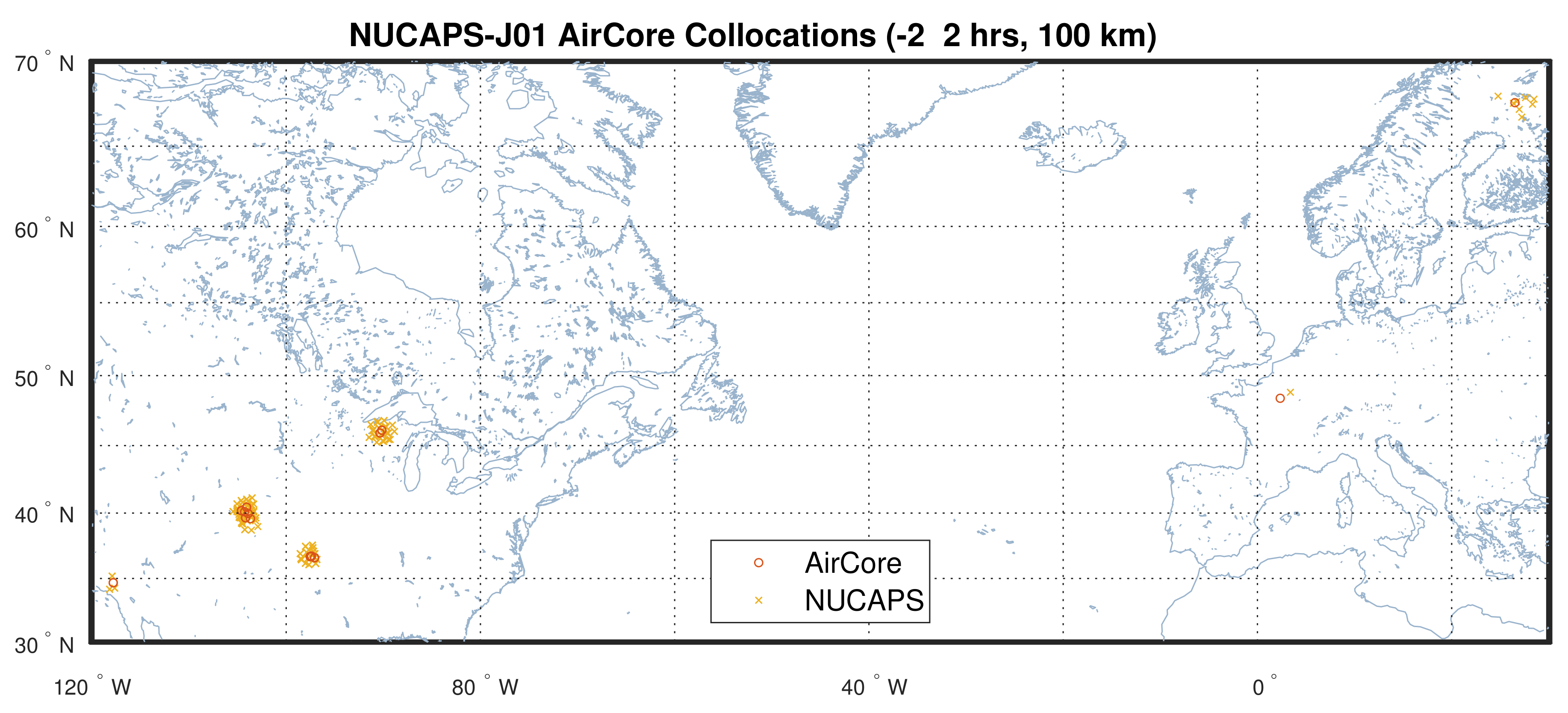
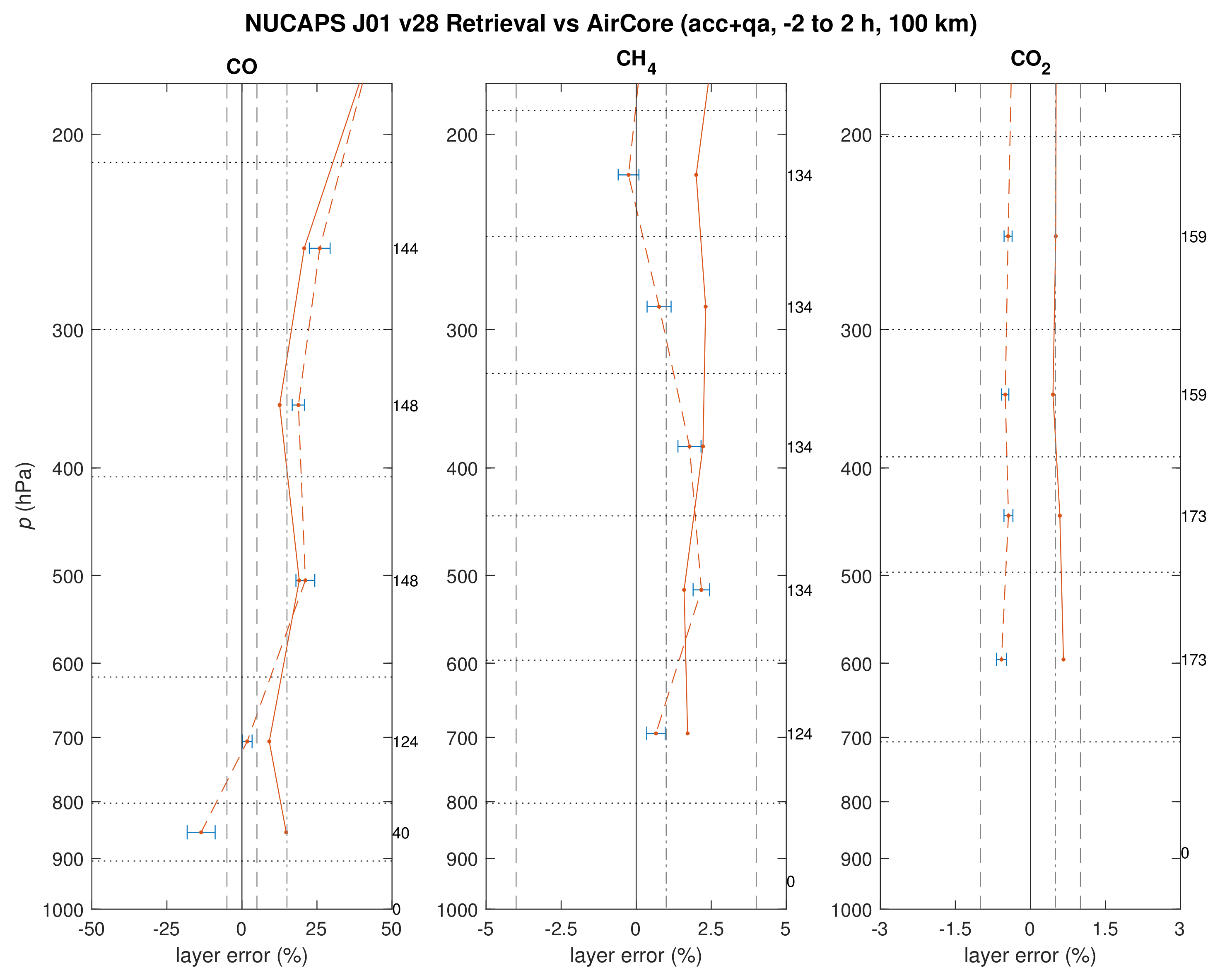
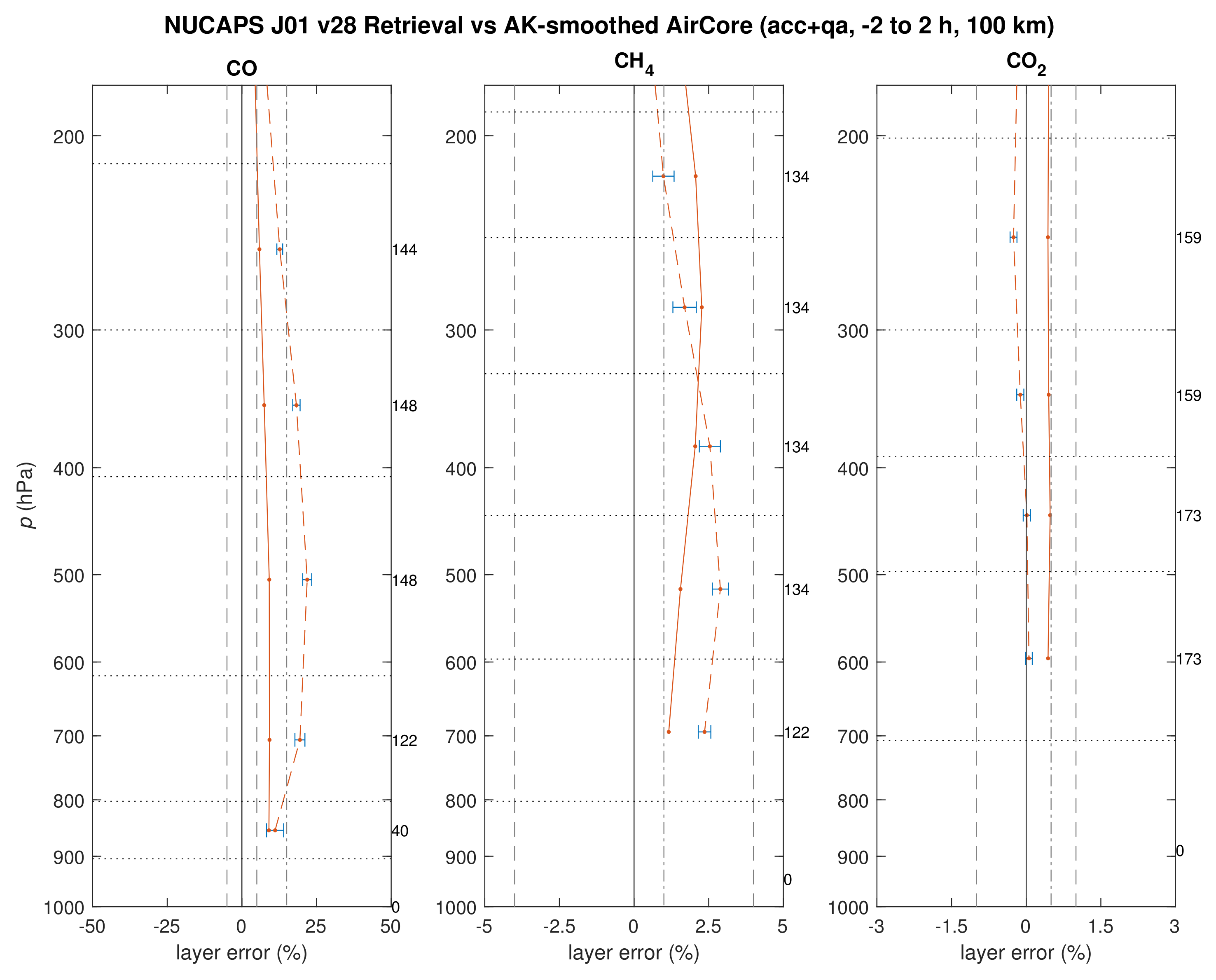
4.2. Statistical Analysis versus AirCore Baseline
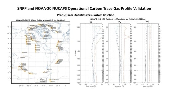
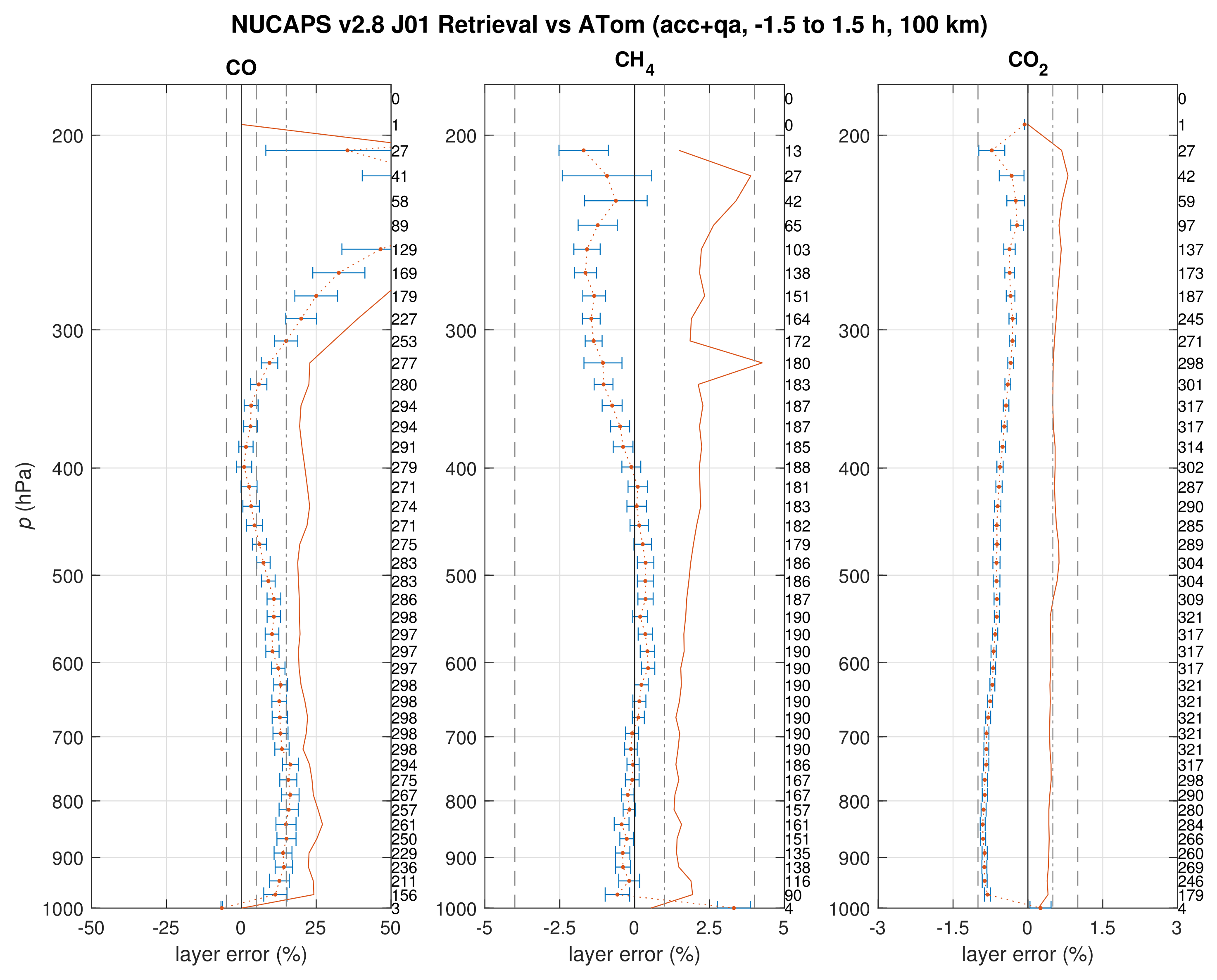
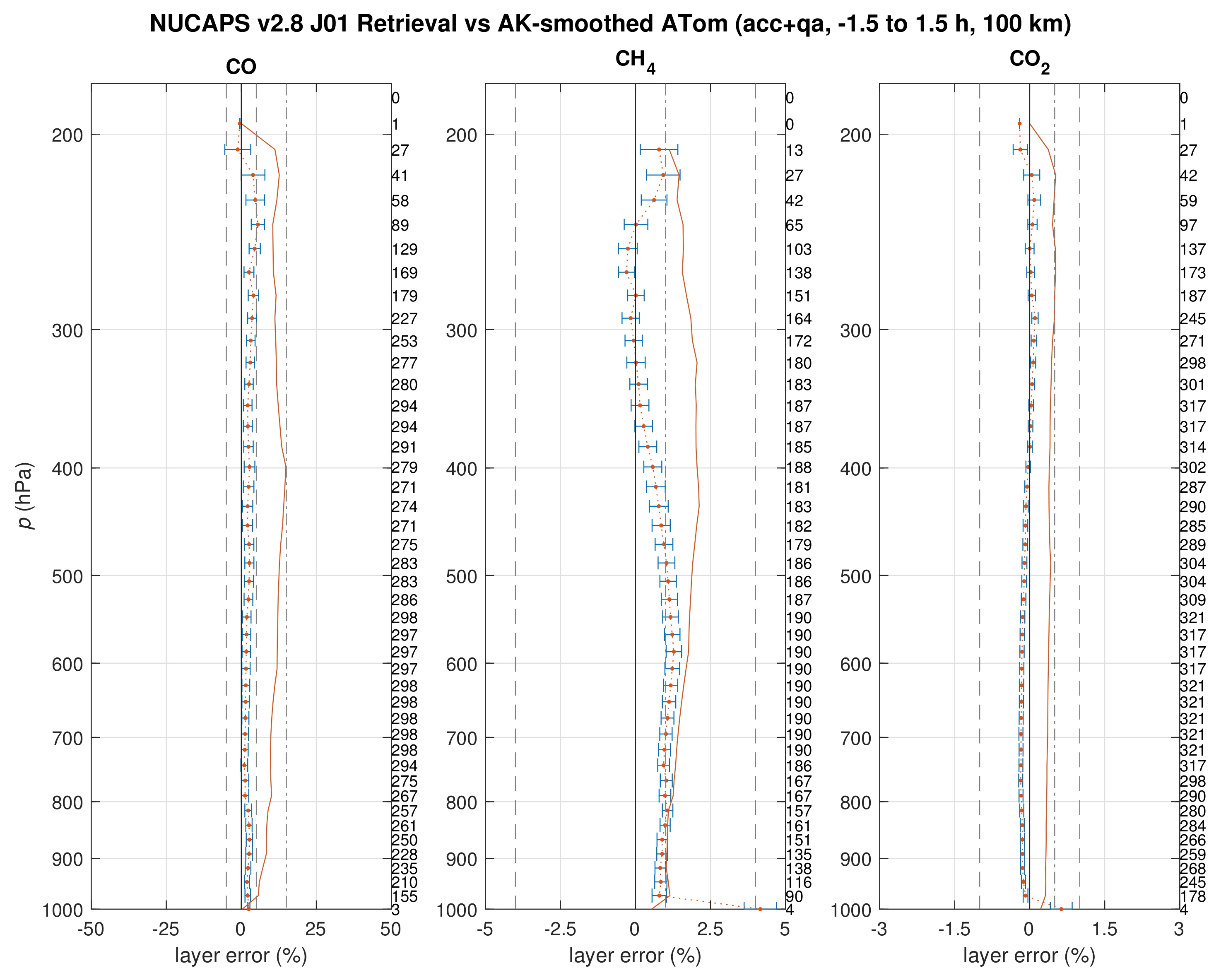
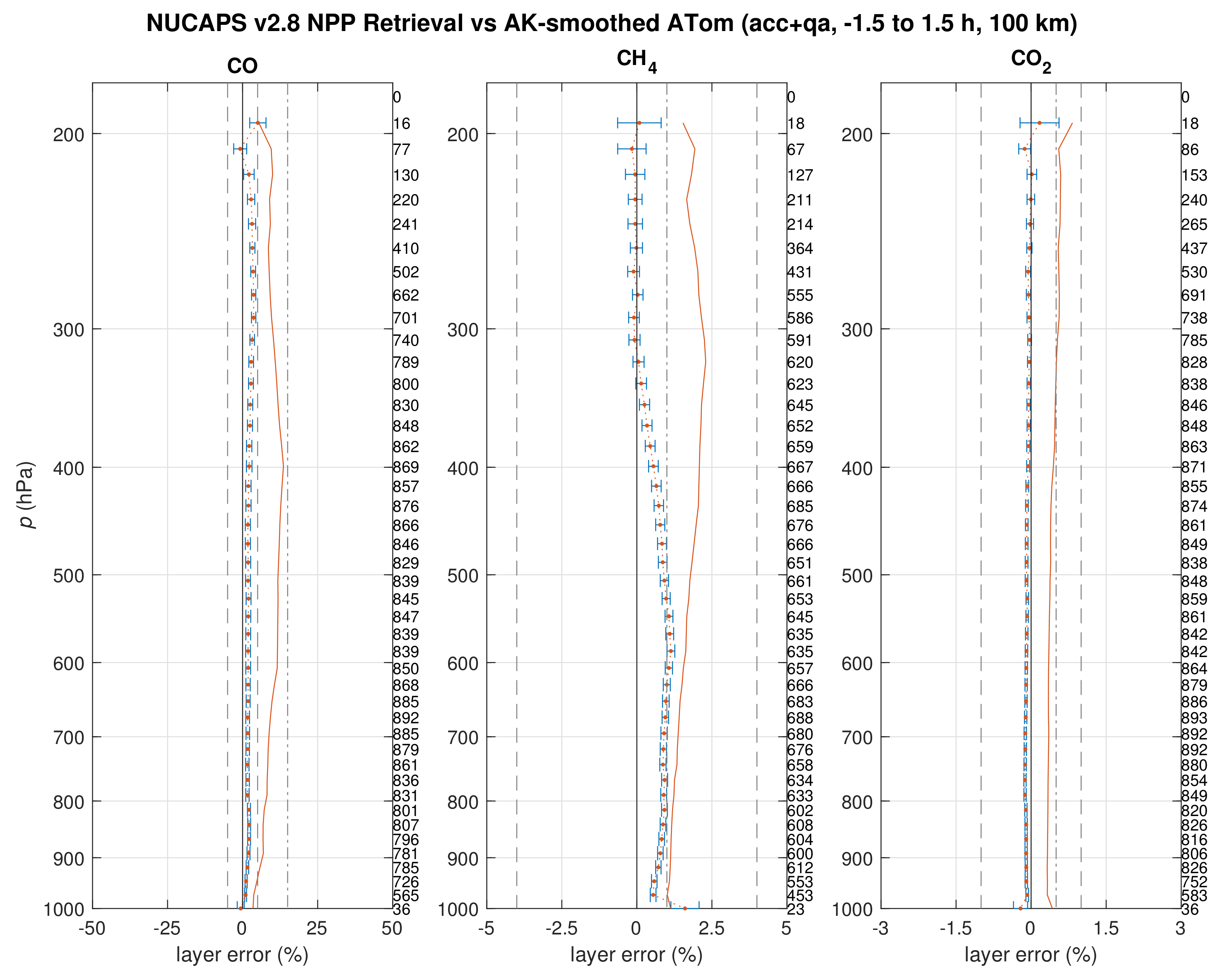
4.3. Statistical Analysis versus ATom Baseline
5. Conclusions and Future Work
Author Contributions
Funding
Acknowledgments
Conflicts of Interest
Abbreviations
| AIRS | Atmospheric Infrared Sounder |
| AK(s) | averaging kernel(s) |
| ATMS | Advanced Technology Microwave Sounder |
| ATom | Atmospheric Tomography mission |
| CAMS | Copernicus Atmosphere Monitoring Service |
| CrIS | Cross-track Infrared Sounder |
| DoF | degrees-of-freedom |
| ECMWF | European Center for Medium Range Weather Forecast |
| EDR(s) | environmental data record(s) |
| EUMETSAT | European Organisation for the Exploitation of Meteorological Satellites |
| FOR(s) | field(s)-of-regard (NUCAPS) |
| FSR | full spectral-resolution (CrIS) |
| FTS | Fourier transform spectrometer |
| IASI | Infrared Atmospheric Sounding Interferometer |
| JPSS | Joint Polar Satellite System |
| J-1 or J01 | JPSS-1 satellite (i.e., NOAA-20 pre-launch, still used as a designator in operational files) |
| LEO | low earth orbit |
| NOAA | National Oceanic and Atmospheric Adminstration |
| NUCAPS | NOAA-Unique Combined Atmospheric Processing System |
| OE | optimal estimation |
| QA | quality assurance |
| RH | relative humidity |
| RMSE | root mean square error |
| RTA | radiative transfer algorithm (alternatively, rapid transmittance algorithm) |
| RTM | radiative transfer model |
| SARTA | Stand-Alone Radiative Transfer Algorithm |
| SDR(s) | sensor data record(s) |
| SNPP | Suomi National Polar-orbiting Partnership (satellite) |
| TCCON | Total Carbon Column Observing Network |
| UT/LS | upper-troposphere/lower-stratosphere |
Appendix A. NUCAPS to TCCON Conversions
Appendix A.1. Column Integration Formulas
Appendix A.2. NUCAPS Layer Conversions
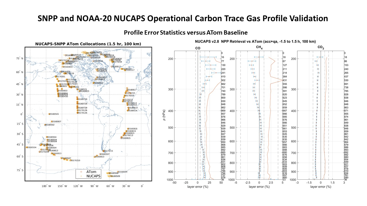
Appendix A.3. Application of TCCON Column AKs
References
- Han, Y.; Revercomb, H.; Cromp, M.; Gu, D.; Johnson, D.; Mooney, D.; Scott, D.; Strow, L.; Bingham, G.; Borg, L.; et al. Suomi NPP CrIS measurements, sensor data record algorithm, calibration and validation activities, and record data quality. J. Geophys. Res. Atmos. 2013, 118, 12734–12748. [Google Scholar] [CrossRef]
- Weng, F.; Zou, X.; Wang, X.; Yang, S.; Goldberg, M.D. Introduction to Suomi national polar-orbiting partnership advanced technology microwave sounder for numerical weather prediction and tropical cyclone applications. J. Geophys. Res. 2012, 117, D19112. [Google Scholar] [CrossRef]
- Han, Y.; Chen, Y. Calibration algorithm for Cross-Track Infrared Sounder full spectral resolution measurements. IEEE Trans. Geosci. Remote Sens. 2018, 56, 1008–1016. [Google Scholar] [CrossRef]
- Cayla, F.R. IASI infrared interferometer for operations and research. In High Spectral Resolution Infrared Remote Sensing for Earth’s Weather and Climate Studies; NATO ASI Series; Chedin, S., Ed.; Springer: Berlin/Heidelberg, Germany, 1993; Volume 19, pp. 9–19. [Google Scholar]
- Hilton, F.; Armante, R.; August, T.; Barnet, C.; Bouchard, A.; Camy-Peyret, C.; Capelle, V.; Clarisse, L.; Clerbaux, C.; Coheur, P.F.; et al. Hyperspectral Earth observation from IASI: Five years of accomplishments. Bull. Am. Meteorol. Soc. 2012, 93, 347–370. [Google Scholar] [CrossRef]
- Aumann, H.H.; Chahine, M.T.; Gautier, C.; Goldberg, M.D.; Kalnay, E.; McMillin, L.M.; Revercomb, H.; Rosenkranz, P.W.; Smith, W.L.; Staelin, D.H.; et al. AIRS/AMSU/HSB on the Aqua Mission: Design, science objectives, data products, and processing systems. IEEE Trans. Geosci. Remote Sens. 2003, 41, 253–264. [Google Scholar] [CrossRef] [Green Version]
- Chahine, M.T.; Pagano, T.S.; Aumann, H.H.; Atlas, R.; Barnet, C.; Blaisdell, J.; Chen, L.; Divakarla, M.; Fetzer, E.J.; Goldberg, M.; et al. AIRS: Improving weather forecasting and providing new data on greenhouse gases. Bull. Am. Meteorol. Soc. 2006, 87, 911–926. [Google Scholar] [CrossRef] [Green Version]
- Gambacorta, A.; Barnet, C.; Wolf, W.; Goldberg, M.; King, T.; Nalli, N.; Maddy, E.; Xiong, X.; Divakarla, M. The NOAA Unique CrIS/ATMS Processing System (NUCAPS): First light retrieval results. In Proceedings of the ITSC-XVIII International TOVS Working Group (ITWG), Toulouse, France, 21–27 March 2012. [Google Scholar]
- Smith, N.; Barnet, C.D. Uncertainty Characterization and Propagation in the Community Long-Term Infrared Microwave Combined Atmospheric Product System (CLIMCAPS). Remote Sens. 2019, 11, 1227. [Google Scholar] [CrossRef] [Green Version]
- Susskind, J.; Barnet, C.D.; Blaisdell, J.M. Retrieval of atmospheric and surface paramaters from AIRS/AMSU/HSB data in the presence of clouds. IEEE Trans. Geosci. Remote Sens. 2003, 41, 390–409. [Google Scholar] [CrossRef]
- Susskind, J.; Blaisdell, J.; Iredell, L.; Keita, F. Improved temperature sounding and quality control methodology using AIRS/AMSU data: The AIRS Science Team version 5 retrieval algorithm. IEEE Trans. Geosci. Remote Sens. 2011, 49, 883–907. [Google Scholar] [CrossRef] [Green Version]
- Han, Y.; Chen, Y.; Xiong, X.; Jin, X. S-NPP CrIS Full Spectral Resolution SDR Processing and Data Quality Assessment; Annual Meeting; American Meteorological Society: Phoenix, AZ, USA, 2015; Available online: https://ams.confex.com/ams/95Annual/webprogram/Paper261524.html (accessed on 28 September 2020).
- Gambacorta, A.; Barnet, C.; Wolf, W.; King, T.; Maddy, E.; Strow, L.; Xiong, X.; Nalli, N.; Goldberg, M. An experiment using high spectral resolution CrIS measurements for atmospheric trace gases: Carbon monoxide retrieval impact study. IEEE Geosci. Remote Sens. Lett. 2014, 11, 1639–1643. [Google Scholar] [CrossRef]
- Strow, L.L.; Hannon, S.E.; Souza-Machado, S.D.; Motteler, H.E.; Tobin, D. An overview of the AIRS Radiative Transfer Model. IEEE Trans. Geosci. Remote Sens. 2003, 41, 303–313. [Google Scholar] [CrossRef] [Green Version]
- Gambacorta, A.; Nalli, N.R.; Barnet, C.D.; Tan, C.; Iturbide-Sanchez, F.; Zhang, K. The NOAA Unique Combined Atmospheric Processing System (NUCAPS): Algorithm Theoretical Basis Document (ATBD); ATBD v2.0; NOAA/NESDIS/STAR Joint Polar Satellite System: College Park, MD, USA, 2017. Available online: https://www.star.nesdis.noaa.gov/jpss/documents/ATBD/ATBD_NUCAPS_v2.0.pdf (accessed on 28 September 2020).
- Gambacorta, A.; Barnet, C. Methodology and information content of the NOAA NESDIS operational channel selection for the Cross-Track Infrared Sounder (CrIS). IEEE Trans. Geosci. Remote Sens. 2013, 51, 3207–3216. [Google Scholar] [CrossRef]
- Warner, J.X.; Wei, Z.; Strow, L.L.; Barnet, C.D.; Sparling, L.C.; Diskin, G.; Sachse, G. Improved agreement of AIRS tropospheric carbon monoxide products with other EOS sensors using optimal estimation retrievals. Atmos. Chem. Phys. 2010, 10, 9521–9533. [Google Scholar] [CrossRef] [Green Version]
- Warner, J.X.; Carminati, F.; Wei, Z.; Lahoz, W.; Attié, J.L. Tropospheric carbon monoxide variability from AIRS under clear and cloudy conditions. Atmos. Chem. Phys. 2013, 13, 12469–12479. [Google Scholar] [CrossRef] [Green Version]
- Xiong, X.; Barnet, C.; Maddy, E.S.; Gambacorta, A.; King, T.S.; Wofsy, S.C. Mid-upper tropospheric methane retrieval from IASI and its validation. Atmos. Meas. Tech. 2013, 6, 2255–2265. [Google Scholar] [CrossRef]
- Maddy, E.S.; Barnet, C.D.; Goldberg, M.; Sweeney, C.; Liu, X. CO2 retrievals from the Atmospheric Infrared Sounder: Methodology and validation. J. Geophys. Res. 2008, 113, D11301. [Google Scholar] [CrossRef] [Green Version]
- Nalli, N.R.; Gambacorta, A.; Liu, Q.; Barnet, C.D.; Tan, C.; Iturbide-Sanchez, F.; Reale, T.; Sun, B.; Wilson, M.; Borg, L.; et al. Validation of atmospheric profile retrievals from the SNPP NOAA-Unique Combined Atmospheric Processing System. Part 1: Temperature and moisture. IEEE Trans. Geosci. Remote Sens. 2018, 56, 180–190. [Google Scholar] [CrossRef]
- Nalli, N.R.; Gambacorta, A.; Liu, Q.; Tan, C.; Iturbide-Sanchez, F.; Barnet, C.D.; Joseph, E.; Morris, V.R.; Oyola, M.; Smith, J.W. Validation of atmospheric profile retrievals from the SNPP NOAA-Unique Combined Atmospheric Processing System. Part 2: Ozone. IEEE Trans. Geosci. Remote Sens. 2018, 56, 598–607. [Google Scholar] [CrossRef]
- Sun, B.; Reale, A.; Tilley, F.; Pettey, M.; Nalli, N.R.; Barnet, C.D. Assessment of NUCAPS S-NPP CrIS/ATMS Sounding Products Using Reference and Conventional Radiosonde Observations. IEEE J. Sel. Top. Appl. Earth Obs. 2017, 10, 2499–2509. [Google Scholar] [CrossRef]
- Feltz, M.L.; Borg, L.; Knuteson, R.O.; Tobin, D.; Revercomb, H.; Gambacorta, A. Assessment of NOAA NUCAPS upper air temperature profiles using COSMIC GPS radio occultation and ARM radiosondes. J. Geophys. Res. Atmos. 2017, 122, 9130–9153. [Google Scholar] [CrossRef]
- Zhou, L.; Divakarla, M.; Liu, X. An Overview of the Joint Polar Satellite System (JPSS) Science Data Product Calibration and Validation. Remote Sens. 2016, 8, 139. [Google Scholar] [CrossRef] [Green Version]
- Nalli, N.R.; Barnet, C.D.; Reale, A.; Tobin, D.; Gambacorta, A.; Maddy, E.S.; Joseph, E.; Sun, B.; Borg, L.; Mollner, A.; et al. Validation of satellite sounder environmental data records: Application to the Cross-track Infrared Microwave Sounder Suite. J. Geophys. Res. Atmos. 2013, 118, 13628–13643. [Google Scholar] [CrossRef]
- Fetzer, E.; McMillin, L.M.; Tobin, D.; Aumann, H.H.; Gunson, M.R.; McMillan, W.W.; Hagan, D.E.; Hofstadter, M.D.; Yoe, J.; Whiteman, D.N.; et al. AIRS/AMSU/HSB validation. IEEE Trans. Geosci. Remote Sens. 2003, 41, 418–431. [Google Scholar] [CrossRef]
- Jacobson, A.R.; Schuldt, K.N.; Miller, J.B.; Oda, T.; Tans, P.; Arlyn, A.; Mund, J.; Ott, L.; Collatz, G.J.; Aalto, T.; et al. CarbonTracker CT2019. 2020. Available online: https://www.esrl.noaa.gov/gmd/ccgg/carbontracker/CT2019/ (accessed on 28 September 2020). [CrossRef]
- Inness, A.; Ades, M.; Agustí-Panareda, A.; Barré, J.; Benedictow, A.; Blechschmidt, A.M.; Dominguez, J.J.; Engelen, R.; Eskes, H.; Flemming, J.; et al. The CAMS reanalysis of atmospheric composition. Atmos. Chem. Phys. 2019, 19, 3515–3556. [Google Scholar] [CrossRef] [Green Version]
- Rodgers, C.D.; Connor, B.J. Intercomparison of remote sounding instruments. J. Geophys. Res. 2003, 108, 4116. [Google Scholar] [CrossRef] [Green Version]
- Wunch, D.; Toon, G.C.; Blavier, J.F.L.; Washenfelder, R.A.; Notholt, J.; Connor, B.J.; Griffith, D.W.T.; Sherlock, V.; Wennberg, P.O. The Total Carbon Column Observing Network. Philos. Trans. R. Soc. A 2011, 369, 2087–2112. [Google Scholar] [CrossRef] [Green Version]
- Karion, A.; Sweeney, C.; Tans, P.; Newberger, T. AirCore: An Innovative Atmospheric Sampling System. J. Atmos. Ocean. Technol. 2010, 27, 1839–1853. [Google Scholar] [CrossRef]
- Membrive, O.; Crevoisier, C.; Sweeney, C.; Danis, F.; Hertzog, A.; Engel, A.; Bönisch, H.; Picon, L. AirCore-HR: A high-resolution column sampling to enhance the vertical description of CH4 and CO2. Atmos. Meas. Tech. 2017, 10, 2163–2181. [Google Scholar] [CrossRef] [Green Version]
- Wofsy, S.; Afshar, S.; Allen, H.; Apel, E.; Asher, E.; Barletta, B.; Bent, J.; Bian, H.; Biggs, B.; Blake, D.; et al. ATom: Merged Atmospheric Chemistry, Trace Gases, and Aerosols. ORNL Distributed Active Archive Center. 2018. Available online: https://daac.ornl.gov/cgi-bin/dsviewer.pl?ds_id=1581 (accessed on 28 September 2020). [CrossRef]
- Wofsy, S.C. HIAPER Pole-to-Pole Observations (HIPPO): Fine-grained, global-scale measurements of climatically important atmospheric gases and aerosols. Philos. Trans. R. Soc. A 2011, 369, 2073–2086. [Google Scholar] [CrossRef]
- Tans, P.P. System and Method for Providing Vertical Profile Measurements of Atmospheric Gases. U.S. Patent 7,597,014, 6 October 2009. [Google Scholar]
- Backus, G.; Gilbert, F. Uniqueness in the Inversion of Inaccurate Gross Earth Data. Philos. Trans. R. Soc. Lond. A Math. Phys. Sci. 1970, 266, 123–192. [Google Scholar] [CrossRef] [Green Version]
- Conrath, B.J. Vertical resolution of temperature profiles obtained from remote radiation measurements. J. Atmos. Sci. 1972, 29, 1262–1271. [Google Scholar] [CrossRef] [Green Version]
- Rodgers, C.D. Characterization and error analysis of profiles retrieved from remote sounding measurements. J. Geophys. Res. 1990, 95, 5587–5595. [Google Scholar] [CrossRef]
- Maddy, E.S.; Barnet, C.D. Vertical resolution estimates in Version 5 of AIRS operational retrievals. IEEE Trans. Geosci. Remote Sens. 2008, 46, 2375–2384. [Google Scholar] [CrossRef]
- Pollard, D.F.; Robinson, J.; Shiona, H. TCCON Data from Lauder (NZ), Release GGG2014.R0. TCCON Data Archive, Hosted by CaltechDATA. 2019. Available online: https://data.caltech.edu/records/1220 (accessed on 28 September 2020). [CrossRef]
- Sherlock, V.; Connor, B.J.; Robinson, J.; Shiona, H.; Smale, D.; Pollard, D. TCCON data from Lauder (NZ), 125HR, Release GGG2014R0. TCCON Data Archive, Hosted By CaltechDATA. 2017. Available online: https://data.caltech.edu/records/281 (accessed on 28 September 2020). [CrossRef]
- Griffith, D.W.; Velazco, V.A.; Deutscher, N.M.; Murphy, C.; Jones, N.; Wilson, S.; Macatangay, R.; Kettlewell, G.; Buchholz, R.R.; Riggenbach, M. TCCON data from Wollongong (AU), Release GGG2014R0. TCCON Data Archive, Hosted by CaltechDATA. 2014. Available online: https://ro.uow.edu.au/data/47/ (accessed on 28 September 2020). [CrossRef]
- Griffith, D.W.; Deutscher, N.M.; Velazco, V.A.; Wennberg, P.O.; Yavin, Y.; Aleks, G.K.; Washenfelder, R.A.; Toon, G.C.; Blavier, J.F.; Murphy, C.; et al. TCCON Data from Darwin (AU), Release GGG2014R0. TCCON Data Archive, Hosted by CaltechDATA. 2017. Available online: https://data.caltech.edu/records/269 (accessed on 28 September 2020). [CrossRef]
- Morino, I.; Velazco, V.A.; Akihiro, H.; Osamu, U.; Griffith, D.W.T. TCCON data from Burgos, Ilocos Norte (PH), Release GGG2014.R0. TCCON Data Archive, Hosted by CaltechDATA. 2018. Available online: https://data.caltech.edu/records/1090 (accessed on 28 September 2020). [CrossRef]
- Blumenstock, T.; Hase, F.; Schneider, M.; Garcia, O.E.; Sepulveda, E. TCCON data from Izana (ES), Release GGG2014R0. TCCON data archive, hosted by CaltechDATA. 2017. Available online: https://data.caltech.edu/records/275 (accessed on 28 September 2020). [CrossRef]
- Kawakami, S.; Ohyama, H.; Arai, K.; Okumura, H.; Taura, C.; Fukamachi, T.; Sakashita, M. TCCON Data from Saga (JP), Release GGG2014R0. TCCON Data Archive, Hosted by CaltechDATA. 2017. Available online: https://data.caltech.edu/records/288 (accessed on 28 September 2020). [CrossRef]
- Iraci, L.T.; Podolske, J.; Hillyard, P.W.; Roehl, C.; Wennberg, P.O.; Blavier, J.F.; Allen, N.; Wunch, D.; Osterman, G.B.; Albertson, R. TCCON Data from Edwards (US), Release GGG2014R1. TCCON Data Archive, Hosted by CaltechDATA. 2017. Available online: https://data.caltech.edu/records/270 (accessed on 28 September 2020). [CrossRef]
- Wennberg, P.O.; Wunch, D.; Roehl, C.; Blavier, J.F.; Toon, G.C.; Allen, N.; Dowell, P.; Teske, K.; Martin, C.; Martin, J. TCCON data from Lamont (US), Release GGG2014R1. TCCON Data Archive, Hosted by CaltechDATA. 2017. Available online: https://data.caltech.edu/records/279 (accessed on 28 September 2020). [CrossRef]
- Morino, I.; Yokozeki, N.; Matzuzaki, T.; Horikawa, M. TCCON data from Rikubetsu (JP), Release GGG2014R2. TCCON Data Archive, Hosted by CaltechDATA. 2017. Available online: https://data.caltech.edu/records/287 (accessed on 28 September 2020). [CrossRef]
- Wennberg, P.O.; Roehl, C.; Wunch, D.; Toon, G.C.; Blavier, J.F.; Washenfelder, R.A.; Keppel-Aleks, G.; Allen, N.; Ayers, J. TCCON data from Park Falls (US), Release GGG2014R0. TCCON Data Archive, Hosted by CaltechDATA. 2017. Available online: https://data.caltech.edu/records/204 (accessed on 28 September 2020). [CrossRef]
- Sussmann, R.; Rettinger, M. TCCON data from Zugspitze (DE), Release GGG2014R1. TCCON Data Archive, Hosted by CaltechDATA. 2018. Available online: https://data.caltech.edu/records/923 (accessed on 28 September 2020). [CrossRef]
- Sussmann, R.; Rettinger, M. TCCON Data from Garmisch (DE), Release GGG2014R0. TCCON Data Archive, Hosted by CaltechDATA. 2014. Available online: https://data.caltech.edu/records/273 (accessed on 28 September 2020). [CrossRef]
- Warneke, T.; Messerschmidt, J.; Notholt, J.; Weinzierl, C.; Deutscher, N.M.; Petri, C.; Grupe, P.; Vuillemin, C.; Truong, F.; Schmidt, M.; et al. TCCON Data from Orléans (FR), Release GGG2014R0. TCCON Data Archive, Hosted by CaltechDATA. 2017. Available online: https://data.caltech.edu/records/283 (accessed on 28 September 2020). [CrossRef]
- Té, Y.; Jeseck, P.; Janssen, C. TCCON Data from Paris (FR), Release GGG2014R0. TCCON Data Archive, Hosted by CaltechDATA. 2017. Available online: https://data.caltech.edu/records/284 (accessed on 28 September 2020). [CrossRef]
- Hase, F.; Blumenstock, T.; Dohe, S.; Gross, J.; Kiel, M. TCCON Data from Karlsruhe (DE), Release GGG2014R1. TCCON Data Archive, Hosted by CaltechDATA. 2017. Available online: https://data.caltech.edu/records/278 (accessed on 28 September 2020). [CrossRef]
- Deutscher, N.M.; Notholt, J.; Messerschmidt, J.; Weinzierl, C.; Warneke, T.; Petri, C.; Grupe, P.; Katrynski, K. TCCON Data from Bialystok (PL), Release GGG2014R1. TCCON Data Archive, Hosted by CaltechDATA. 2017. Available online: https://data.caltech.edu/records/267 (accessed on 28 September 2020). [CrossRef]
- Wunch, D.; Mendonca, J.; Colebatch, O.; Allen, N.; Blavier, J.F.L.; Roche, S.; Hedelius, J.K.; Neufeld, G.; Springett, S.; Worthy, D.E.J.; et al. TCCON Data from East Trout Lake (CA), Release GGG2014R1. TCCON Data Archive, Hosted by CaltechDATA. 2017. Available online: https://data.caltech.edu/records/362 (accessed on 28 September 2020). [CrossRef]
- Kivi, R.; Heikkinen, P.; Kyrö, E. TCCON Data from Sodankyla (FI), Release GGG2014R0. TCCON Data Archive, Hosted by CaltechDATA. 2017. Available online: https://data.caltech.edu/records/289 (accessed on 28 September 2020). [CrossRef]
- Kivi, R.; Heikkinen, P. Fourier transform spectrometer measurements of column CO2 at Sodankylä, Finland. Geosci. Instrum. Method. Data Syst. 2016, 5, 271–279. [Google Scholar] [CrossRef] [Green Version]
- Notholt, J.; Warneke, T.; Petri, C.; Deutscher, N.M.; Weinzierl, C.; Palm, M.; Buschmann, M. TCCON data from Ny Ålesund, Spitsbergen (NO), Release GGG2014.R0. TCCON Data Archive, Hosted by CaltechDATA. 2017. Available online: https://data.caltech.edu/records/301 (accessed on 28 September 2020). [CrossRef]
- Hedelius, J.K.; He, T.L.; Jones, D.B.A.; Baier, B.C.; Buchholz, R.R.; De Mazière, M.; Deutscher, N.M.; Dubey, M.K.; Feist, D.G.; Griffith, D.W.T.; et al. Evaluation of MOPITT Version 7 joint TIR–NIR XCO retrievals with TCCON. Atmos. Meas. Tech. 2019, 12, 5547–5572. [Google Scholar] [CrossRef] [Green Version]
- Wennberg, P.O.; Wunch, D.; Roehl, C.; Blavier, J.F.; Toon, G.C.; Allen, N. TCCON Data from Caltech (US), Release GGG2014R1. TCCON Data Archive, Hosted by CaltechDATA. 2017. Available online: https://data.caltech.edu/records/285 (accessed on 28 September 2020). [CrossRef]
- Wennberg, P.O.; Roehl, C.; Blavier, J.F.; Wunch, D.; Landeros, J.; Allen, N. TCCON Data from Jet Propulsion Laboratory (US), 2011, Release GGG2014R1. TCCON Data Archive, Hosted by CaltechDATA. 2017. Available online: https://data.caltech.edu/records/277 (accessed on 28 September 2020). [CrossRef]
- Notholt, J.; Petri, C.; Warneke, T.; Deutscher, N.M.; Buschmann, M.; Weinzierl, C.; Macatangay, R.; Grupe, P. TCCON Data from Bremen (DE), Release GGG2014R0. TCCON Data Archive, Hosted by CaltechDATA. 2017. Available online: https://data.caltech.edu/records/268 (accessed on 28 September 2020). [CrossRef]
- Strong, K.; Mendonca, J.; Weaver, D.; Fogal, P.; Drummond, J.; Batchelor, R.; Lindenmaier, R. TCCON Data from Eureka (CA), Release GGG2014R1. TCCON Data Archive, Hosted by CaltechDATA. 2017. Available online: https://data.caltech.edu/records/271 (accessed on 28 September 2020). [CrossRef]
- Nalli, N.R.; Joseph, E.; Morris, V.R.; Barnet, C.D.; Wolf, W.W.; Wolfe, D.; Minnett, P.J.; Szczodrak, M.; Izaguirre, M.A.; Lumpkin, R.; et al. Multi-year observations of the tropical Atlantic atmosphere: Multidisciplinary applications of the NOAA Aerosols and Ocean Science Expeditions (AEROSE). Bull. Am. Meteorol. Soc. 2011, 92, 765–789. [Google Scholar] [CrossRef] [Green Version]
- Nalli, N.R.; Barnet, C.D.; Reale, T.; Liu, Q.; Morris, V.R.; Spackman, J.R.; Joseph, E.; Tan, C.; Sun, B.; Tilley, F.; et al. Satellite sounder observations of contrasting tropospheric moisture transport regimes: Saharan air layers, Hadley cells, and atmospheric rivers. J. Hydrometeorol. 2016, 17, 2997–3006. [Google Scholar] [CrossRef]
- Le Marshall, J.; Jung, J.; Goldberg, M.; Barnet, C.; Wolf, W.; Derber, J.; Treadon, R.; Lord, S. Using cloudy AIRS fields of view in numerical weather prediction. Aust. Met. Mag. 2008, 57, 249–254. [Google Scholar]
- Wunch, D.; Toon, G.C.; Wennberg, P.O.; Wofsy, S.C.; Stephens, B.B.; Fischer, M.L.; Uchino, O.; Abshire, J.B.; Bernath, P.; Biraud, S.C.; et al. Calibration of the Total Carbon Column Observing Network using aircraft profile data. Atmos. Meas. Tech. 2010, 3, 1351–1362. [Google Scholar] [CrossRef] [Green Version]


| Statistic | Threshold | Objective |
|---|---|---|
| Carbon Monoxide EDR | ||
| CO Precision † | 15% | 3% |
| CO Accuracy ‡ | ±5% | ±5% |
| Methane EDR | ||
| CH4 Precision | 1% (20 ppbv) | N/A |
| CH4 Accuracy | ±4% (80 ppbv) | N/A |
| Carbon Dioxide EDR | ||
| CO2 Precision | 0.5% (2 ppmv) | 1.05 to 1.4 ppmv |
| CO2 Accuracy | ±1% (4 ppmv) | N/A |
| Trace Gas | Bias (%) | σ (%) | RMSE (%) | r | p | N | Yield | |||||
|---|---|---|---|---|---|---|---|---|---|---|---|---|
| Raw | AK | Raw | AK | Raw | AK | Raw | AK | Raw | AK | |||
| NOAA-20 | ||||||||||||
| CO | +10.5 | +2.0 | 18.6 | 9.6 | 21.4 | 9.8 | 0.92 | 0.92 | 0 | 0 | 298 | 59% |
| CH4 | −0.2 | +0.8 | 1.4 | 1.3 | 1.4 | 1.6 | 0.61 | 0.61 | 0 | 0 | 190 | 38% |
| CO2 | −0.7 | −0.1 | 0.4 | 0.3 | 0.8 | 0.3 | 0.81 | 0.84 | 0 | 0 | 321 | 63% |
| Suomi NPP | ||||||||||||
| CO | +7.8 | +1.9 | 15.6 | 8.3 | 17.5 | 8.5 | 0.91 | 0.89 | 0 | 0 | 901 | 64% |
| CH4 | +0.0 | +0.7 | 1.6 | 1.3 | 1.6 | 1.5 | 0.38 | 0.38 | 0 | 0 | 696 | 49% |
| CO2 | −0.6 | −0.1 | 0.4 | 0.3 | 0.7 | 0.3 | 0.78 | 0.79 | 0 | 0 | 969 | 69% |
© 2020 by the authors. Licensee MDPI, Basel, Switzerland. This article is an open access article distributed under the terms and conditions of the Creative Commons Attribution (CC BY) license (http://creativecommons.org/licenses/by/4.0/).
Share and Cite
Nalli, N.R.; Tan, C.; Warner, J.; Divakarla, M.; Gambacorta, A.; Wilson, M.; Zhu, T.; Wang, T.; Wei, Z.; Pryor, K.; et al. Validation of Carbon Trace Gas Profile Retrievals from the NOAA-Unique Combined Atmospheric Processing System for the Cross-Track Infrared Sounder. Remote Sens. 2020, 12, 3245. https://doi.org/10.3390/rs12193245
Nalli NR, Tan C, Warner J, Divakarla M, Gambacorta A, Wilson M, Zhu T, Wang T, Wei Z, Pryor K, et al. Validation of Carbon Trace Gas Profile Retrievals from the NOAA-Unique Combined Atmospheric Processing System for the Cross-Track Infrared Sounder. Remote Sensing. 2020; 12(19):3245. https://doi.org/10.3390/rs12193245
Chicago/Turabian StyleNalli, Nicholas R., Changyi Tan, Juying Warner, Murty Divakarla, Antonia Gambacorta, Michael Wilson, Tong Zhu, Tianyuan Wang, Zigang Wei, Ken Pryor, and et al. 2020. "Validation of Carbon Trace Gas Profile Retrievals from the NOAA-Unique Combined Atmospheric Processing System for the Cross-Track Infrared Sounder" Remote Sensing 12, no. 19: 3245. https://doi.org/10.3390/rs12193245