Article

Precipitation Type Classification of Micro Rain Radar Data Using an Improved Doppler Spectral Processing Methodology

1
Department Applied Physics—Meteorology, Universitat de Barcelona, 08028 Barcelona, Spain
2
SARTI, Universitat Politècnica de Catalunya, 08800 Vilanova i la Geltrú, Spain
3
DT Catalonia, AEMET, 08005 Barcelona, Spain
4
Laboratory of Aerology, University of Toulouse/CNRS, 31400 Toulouse, France
*
Author to whom correspondence should be addressed.
Remote Sens. 2020, 12(24), 4113; https://doi.org/10.3390/rs12244113
Submission received: 17 November 2020 / Revised: 13 December 2020 / Accepted: 14 December 2020 / Published: 16 December 2020
(This article belongs to the Special Issue Estimating Meteorological Variables by Remote Sensing Data)

Abstract

:
This paper describes a methodology for processing spectral raw data from Micro Rain Radar (MRR), a K-band vertically pointing Doppler radar designed to observe precipitation profiles. The objective is to provide a set of radar integral parameters and derived variables, including a precipitation type classification. The methodology first includes an improved noise level determination, peak signal detection and Doppler dealiasing, allowing us to consider the upward movements of precipitation particles. A second step computes for each of the height bin radar moments, such as equivalent reflectivity (Ze), average Doppler vertical speed (W), spectral width (σ), the skewness and kurtosis. A third step performs a precipitation type classification for each bin height, considering snow, drizzle, rain, hail, and mixed (rain and snow or graupel). For liquid precipitation types, additional variables are computed, such as liquid water content (LWC), rain rate (RR), or gamma distribution parameters, such as the liquid water content normalized intercept (Nw) or the mean mass-weighted raindrop diameter (Dm) to classify stratiform or convective rainfall regimes. The methodology is applied to data recorded at the Eastern Pyrenees mountains (NE Spain), first with a detailed case study where results are compared with different instruments and, finally, with a 32-day analysis where the hydrometeor classification is compared with co-located Parsivel disdrometer precipitation-type present weather observations. The hydrometeor classification is evaluated with contingency table scores, including Probability of Detection (POD), False Alarm Rate (FAR), and Odds Ratio Skill Score (ORSS). The results indicate a very good capacity of Method3 to distinguish rainfall and snow (PODs equal or greater than 0.97), satisfactory results for mixed and drizzle (PODs of 0.79 and 0.69) and acceptable for a reduced number of hail cases (0.55), with relatively low rate of false alarms and good skill compared to random chance in all cases (FAR < 0.30, ORSS > 0.70). The methodology is available as a Python language program called RaProM at the public github repository.

Graphical Abstract

1. Introduction

Precipitation is a key component of the hydrological cycle and a precise knowledge of the precipitating hydrometeor type is essential for remote quantitative precipitation estimates either from scanning or from vertically pointing ground-based or spaceborne radars. Precipitation observations of vertically pointing Doppler radars allow us to estimate the fall speed of hydrometeor particles which, in general, are the sum of their terminal fall speed and vertical air velocity (Atlas et al. [1], Hauser and Amayenc [2]). As it is well known, radar sensitivity to smaller particle detection increases with shorter wavelengths but, on the other hand, attenuation by intense precipitation, particularly rainfall, increases. Thus, a compromise exists between sensitivity and attenuation effects regarding the choice of operating frequency, a crucial aspect in radar design for different applications and platforms (Battaglia et al. [3], Kollias et al. [4]).
Unlike usual ground-based scanning precipitation weather radars operating at cm frequencies (S, C or X-band), Doppler radar profilers do not provide the precipitation field over a wide area, but a high spatial and temporal resolution vertical profile over the radar location. This approach has been employed for decades to study fine-scale vertical precipitation characteristics, for instance with the NOAA Aeronomy Laboratory S-band Doppler profiler (Ecklund et al. [5]), the X-band Precipitation Occurrence Sensor System (POSS, Sheppard [6]), the K-band Micro Rain Radar (MRR, Löffler-Mang et al. [7], Peters et al. [8]), and more recently, with shorter wavelength radars traditionally used for cloud studies, such as the Ka-band ARM zenith radar (Chandra et al. [9]) or the Milešovka observatory Ka-band cloud radar (Sokol et al. [10,11]), used to derive a hydrometeor classification, including four precipitation types. A related application has been the use of lidar observations from the NASA MPLNET network to resolve weak precipitation profiles (Lolli et al. [12,13]), particularly suited for light rain, drizzle and virga, as if more intense precipitation exists, attenuation becomes too important.
Among the above-mentioned Doppler radar profilers, the MRR stands out. This has been extensively used for a wide range of applications, including microphysical analysis of rainfall characteristics using collocated ground disdrometers (Adirosi et al. [14,15], Chang et al. [16], Gonzalez et al. [17], Jass et al. [18], Luo et al. [19], Tokay et al. [20]), diurnal and precipitation characteristics at low-latitude mountains (Bendix et al. [21], Seidel et al. [22]), orographic effects and low-level seeder-feeder processes (Arulraj and Barros [23]), bright-band (BB) radar signatures (Cha et al. [24], Brast and Markmann [25]), or the monitoring of absolute calibration of C-band polarimetric weather radars (Frech et al. [26]). Many of these applications rely on the separation of the liquid to solid precipitation phase, for example above and below the BB, which is crucial for accurate quantitative precipitation estimates (Fabry and Zawadzki [27], Sanchez-Diezma et al. [28], Bordoy et al. [29]). A recent study by Makino et al. [30] described the use of MRR to predict the hydrometeor type at ground level. However, to our best knowledge, no methodology based on MRR data to partition precipitation profiles in different hydrometeor types has yet been described. Such methodologies have been developed and improved in recent years for polarimetric scanning precipitation radars (see, for instance, Ryzhkov et al. [31], Park et al. [32], Schuur et al. [33], Dolan et al. [34], Chandrasekar et al. [35], Besic et al. [36]).
MRR units produce so-called raw data files, with spectral Doppler density data, which may be processed with the MRR manufacturer software (Metek [37], hereafter Method1) to obtain derived products, such as radar reflectivity Z, Doppler fall speed w or spectral width σ. Alternatively, researchers may develop their own MRR raw data processing, such as the methodology by Maahn and Kollias [38] which improves sensitivity and Doppler dealiasing and is suited for snowfall precipitation. This methodology is freely available as a Python program, called ImproToo (hereafter Method2).
The objective of this article is threefold. First, to present a novel MRR processing methodology, called RaProM (hereafter Method3), which includes enhanced spectral processing and Doppler dealiasing, a simplified novel hydrometeor classification scheme based on the assumption that the air vertical velocity is negligible compared to the precipitation particle speed, including drizzle, rain, snow, and hail, plus additional variables depending on the precipitation type. Second, to illustrate the methodology with a detailed case study, where results are compared with those from Method1 and Method2 and other co-located instruments, such as a Particle Size and Velocity (Parsivel) disdrometer or a microwave radiometer. Third, an evaluation of the hydrometeor type classification at the lowest MRR height bin compared with Parsivel present weather precipitation type observations recorded in 32 days.
The rest of the article is organized as follows. Section 2 introduces the instruments and location considered in this study, on the Eastern Pyrenees (NE Spain). Section 3 describes the new methodology proposed, dealing with spectral data processing with a multi peak detection procedure and details the derivation of spectral moments, hydrometeor classification and derived parameters. Section 4 presents a case study comparing, in detail, previous MRR processing methodologies and data from additional instruments and also provides the evaluation of the hydrometeor precipitation classification using contingency table scores and, finally, Section 5 presents a discussion and conclusion of the achievements and limitations of the proposed methodology and ideas for further research.

2. Instruments and Site Description

A Micro Rain Radar (MRR) is a compact frequency modulated continuous wave (FMCW) vertically pointing Doppler radar operating at 24.23 GHz, manufactured by Meteorologische Messtechnik GmbH (Metek) [37], which recently is manufacturing a newer version, the MRR-PRO. A summary of technical features of the MRR used here is given in Table 1. In this study, an MRR2 model was used and the range gate resolution was set to 100 m so observations extended up to 3.1 km above ground level. The unit was equipped with a heated antenna which prevented the accumulation of snow. Due to the relatively high operating frequency, possible attenuation by precipitation had to be checked for the data set analyzed.
Other instruments used here were a laser-optical disdrometer OTT Parsivel, a microwave radiometer RPG HATPRO (MWR) and two Automatic Weather Stations (AWSs) of the Meteorological Service of Catalonia [39]—see Supplementary Materials Table S1. All these instruments were deployed for the Cerdanya-2017 field campaign at the Das aerodrome (OACI code: LECD) in the Eastern Pyrenees mountain massif from December 2016 to April 2017. Part of the study makes use of additional data collected at the same site during the period 2018 and 2019 by the MRR and Parsivel disdrometer. The location is a relatively wide valley oriented west to east, with limited radar coverage due to orographic beam blockage (Bech et al. [40], Trapero et al. [41]) so most of the MRR beam cannot be directly compared with existing ground-based weather radar observations. The Cerdanya-2017 field campaign aimed at studying various complex terrain phenomena, including cold pool formation, mountain waves and orographic precipitation—see Gonzalez et al. [17]; Udina et al. [42] for more details.
The disdrometer records hydrometeor fall speed and size spectra at ground level and other derived variables, such as hydrometeor type (e.g., rain or snow), radar reflectivity factor and precipitation intensity for liquid precipitation, among others. The microwave radiometer provides air temperature vertical profiles so the freezing level and other isotherm levels can be calculated. The two AWS are located close or near the MRR location (at the same aerodrome and nearby but a higher altitude, see Figure S1 in Supplementary Materials) and provide independent measurements of temperature, precipitation and snow depth level.

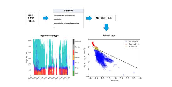
3. New Methodology Proposed

The methodology has two different sections. The spectral data processing is detailed in the first section, and the equations and hypotheses are treated in the second section.

3.1. Spectral Data Processing

The initial processing stage of Method3 consists in the MRR spectral data processing and follows the flow chart described in Figure 1. The first step is to transform the original signal backscattered by hydrometeors to spectral reflectivity (ƞ) following the equation proposed by the manufacturer (Metek [37]):
η ( n , i ) = f ( n , i ) · i 2 T F ( i ) · C · Δ h 10 20   ,
where i is the range gate number (i = 0, …, 31), n is Doppler bin number (n = 0, …, 63), f(n,i) is the original MRR signal saved in the so-called raw data files, TF(i) is a transfer function specific for each height, C is the radar calibration constant and Δh is the range resolution in m. The spectral reflectivity ƞ(n,i) has units of m−1 and TF(i) and C are stored in the original raw data files.
The innovations introduced in Method3 are the modification of the integration time, the average of spectra and the determination of maxima (peaks) in the signal. The integration time, usually set to 60 s, is now selectable by the user. Method3 performs the averaging of the spectrum checking that at least 50% of spectra contain a minimum valid signal. The 50% threshold is a value modifiable by the user on the code of Method3. The signal is considered valid if it verifies the Hildebrand and Sekhon [43] criterion:
η ¯ 2 v a r ( η )   =   ( η ( n ) N ) 2 ( η η ¯ ) 2 N < 60   ,
where var(ƞ) is the spectral reflectivity variance and N the number of Doppler bins considered.
The detection of the maxima of the signal at a given height consists in using all Doppler bins of the spectrum except the first and the last one, therefore all possible fall speed values are used, except the lowest and the highest. This approach allows us to recover more than one single peak of the signal more easily and provides more detail about the hydrometeor fall speed distribution potentially affected by noise in the lowest range bin, the closest one to the ground, which is excluded, as in Method1. Note that Method2, instead, excludes part of the highest and lowest Doppler bins, and discards the 3 lowest-range bins. The noise level is calculated for each height following the scheme detailed by the manufacturer [37], which implies subtracting the noise level to the signal.
Figure 2 shows two examples of noise subtraction and peak detection using Method3 applied to the lowest processed range bin (i = 1, here from 100 to 200 m a.g.l.) and the ninth range bin (i = 10, from 900 to 1000 m a.g.l.). Figure 2a,b display a single peak detection and Figure 2c,d a two peak detection. Note that these detections could not be possible with Method2, as it discards the 100 m to 200 m bin height (panels a and b) and does not consider all Doppler bins processed by Method3.
The next step is the conversion of the reflectivity spectra from n Doppler bins to velocity v according to Equation (3). Note that this transformation depends on specific MRR2 data acquisition features, such as wavelength or sampling frequency:
η ( v , i )   =   η ( n , i ) · ( f s a m p l i n g 2 · n m a x · i m a x · λ 2 ) 1 ,
where fsampling is 125 kHz, nmax is 64, imax is 32 and λ is the wavelength (~1.24 cm).
The last step in the spectral processing of Method3 implements a dealiasing scheme, partly based on Kneifel et al. [44] who noticed that in some snowfall cases, MRR2 provided unrealistically high values of hydrometeor fall speed, much higher than terminal snowflake fall speeds. This was due to two assumptions of the original manufacturer software: (i) precipitation observed was always in liquid form, so there was an inherent dependence between hydrometeor terminal fall speed versus particle diameter and (ii) only downward velocities were allowed, which is the most usual situation but is not always the case for snowflakes or convective rainfall. The snowfall case is discussed in Maahn and Kollias [38] and a dealiasing system to solve it is implemented in Method2. The dealiasing scheme proposed in Method3 consists in, for a given height, combining information from spectra of adjacent (upper and lower) height levels to determine the hydrometeors’ fall speeds to extend the original speed range from 0 to 12 m/s to a dealiased range of −12 to 24 m/s. The lower-level spectra are used to expand the speed range to −12 to 0 m/s and the upper one to 12 to 24 m/s. The vertical continuity of the speed profile is used to provide the dealiased speed spectra, as illustrated in the example displayed in Figure 3. The Method2 dealiasing scheme works well for snowfall and finds possible snowflake upward movements but does not work properly for cases of intense rainfall with hydrometeor falling velocities greater than 8 m/s, unlike the proposed scheme implemented in Method3.

3.2. Parameters Calculation

Once Method3 spectral processing is completed, data are ready to proceed with the calculation of subsequent parameters, which is divided in two parts. The first part computes the basic Doppler radar parameters: the Doppler velocity, which is assumed here to be the hydrometeor fall speed, and the radar equivalent reflectivity factor. The second part provides an estimation of hydrometeor type and based on this, the calculation of derived parameters, such as precipitation rates for different precipitation types. Figure 4 provides an overview of parameters calculations.

3.2.1. Basic Parameters

The term basic parameters are applied here to integral parameters which can be calculated independent of the type of hydrometeor as they only depend on the spectral reflectivity. The parameters are the radar equivalent reflectivity (Ze), the Doppler velocity, which here corresponds to the mean fall speed of hydrometeors ( w ¯ ), and higher order moments of the Doppler speed distributions: Doppler spectral width (σ), skewness and kurtosis as described in Equations (4)–(8):
Z e   =   10 18 · λ 4 π 5 · 1 | K | 2 · Δ v · η ( v ) ,
w ¯   =   η ( v , i ) · v ( i ) η ( v , i )  
σ   =   η ( v , i ) · ( v ( i ) w ) 2 η ( v , i )
s k e w n e s s   =   η ( v , i ) · ( v ( i ) w ) 3 η ( v , i ) · σ 3  
k u r t o s i s   =   η ( v , i ) · ( v ( i ) w ) 4 η ( v , i ) · σ 4  
Note that the calculation of the radar equivalent reflectivity does not take into account possible attenuation effects which may be relevant for high precipitation rates, considering that MRR operates at the K-band. However, this can be handled in the case of liquid hydrometeors, where the path attenuation is calculated (see Section 3.2.4).

3.2.2. Hydrometeor Type Classification

As mentioned earlier, there are a number of hydrometeor classification algorithms developed mainly for scanning polarimetric weather radars, some considering up to 10 different precipitation species. Here, a simplified approach is adopted aiming to distinguish, for each height bin, 5 possible precipitation types: drizzle, rain, snow, mixed and hail. For the purpose of this paper, we consider either wet snow, a mixture of snow and rain, or graupel in the mixed category.
The classification is based on a decision tree, considering empirical relations between hydrometeor fall speed and equivalent radar reflectivity, size and particle diameter characteristics for different hydrometeors and the existence or absence of the bright band. As a starting point, the empirical relations reported by Atlas et al. [1], linking radar reflectivity and fall speeds of rain (vRain) and snow (vSnow) in the absence of bright band, are considered:
v R a i n   =   2.65 · Z e 0.114  
v S n o w = 0.817 · Z e 0.063  
These relationships are used to compute, given Ze, vRain and vSnow, which are the average fall speed expected for each precipitation type on those two cases. Additional parameters considered are the mean Doppler fall speed w ¯ , the Doppler spectral width σ and the Skewness Sk, calculated for each height bin. Moreover, a BB detection scheme is used (Cha et al. [24]). In case there is BB, then the existence and height of its top (BBTop) and bottom (BBBottom) levels are computed, following the methodology described by Wang et al. [45]. From all the above, the decision tree can be grouped in three main branches with additional conditions (Figure 4):
  • If vSnow is within the interval w ¯ ± σ and vRain exceeds w ¯ + σ, then:
    • If the bin height is lower than the BBBottom, the hydrometeor is classified as:
      Drizzle/Rain—Hail.
    • If the bin height is equal or above the BBBottom or BBBottom is not present:
      Mixed: if Sk > −0.5 and w ¯ vSnow;
      Snow: otherwise.
  • If vRain and vSnow are within the interval w ¯ ± σ, then:
    • If the bin height is below the BBBottom or BBBottom is not present:
      Drizzle/Rain—Hail.
    • If the bin height is above the BBBottom:
      Mixed: if the Sk > −0.5 and the w ¯ vSnow;
      Snow: otherwise.
  • If vRain is within the interval w ¯ ± σ and vSnow is lower than w ¯ σ, then:
    • If the bin height is below the BBTop or BBTop is not present:
      Drizzle/Rain—Hail.
    • If the bin height is above the BBTop:
      Mixed: if the Sk > −0.5 and the w ¯ vSnow;
      Snow: otherwise.
  • Cases not included in any of the previous categories are labelled as unknown.
The category “Drizzle/Rain—Hail” is further disaggregated considering additional conditions (Figure 5). The basic criteria stem from the precipitation hydrometeor definitions. Drizzle and rain are formed only by liquid particles AMS (2020) [46,47] and are here distinguished by their skewness Sk in their fall speed distribution and for Ze differences (ΔZe) between levels. According to Acquistapace et al. [48], if skewness (Sk) is lower than or equal to −0.5 and ΔZe ≥ 1 dBZ, then the hydrometeor is classified as drizzle and otherwise as rain. Hail is defined in the function of the maximum diameter on the Doppler velocity spectrum, considering here a threshold of maximum diameters greater than 5 mm. Snow and mixed class are stratified when the height is below the BBBottom as described by Kalesse et al. [49].

3.2.3. Snowfall Rate

Despite solid precipitation presents a greater variability than liquid precipitation, Matrosov and Heymsfield [50] studied the relation between equivalent radar reflectivity and snowfall rate at different wavelengths and proposed empirical relations between those variables. In particular, snowfall rate (SR) can be estimated from Ze by inverting the ZeSR power–law relationship:
S R = ( Z e a ) 1 / b
where SR is in mm/h, Ze in mm6 m−3, a and b are the coefficients from the corresponding ZeSR relation and their values, for K band, are 56.00 and 1.20. It should be noted that the estimated SR might differ from actual values, given the high variability of the mass–size relation of different snow particles, as discussed in Souverijns et al. [51].

3.2.4. Rainfall Parameters from Drizzle/Rain

Rainfall parameters can be calculated if hydrometeors are in liquid phase. Section 3.2.2 details that the Drizzle/Rain types are liquid hydrometeors, thus on these types the rainfall parameters are calculated, but it is also necessary to introduce a dependence between the hydrometeor terminal fall speed and the diameter of the hydrometeor, which implies the hydrometeor particle size distribution (N) for each n Doppler bin and height level i:
N n , i ( D n )   =   η ( D ) σ n , i  
where ƞ(D) is the spectral reflectivity as a function of the diameter and σn,i is the Mie backscattering cross section for liquid spherical particles. Note that the initial spectral reflectivity is only a function of the fall speed using the relation between Doppler bins n. The spectral reflectivity as a function of the raindrop diameter is determined using the Gunn and Kinzer [52] expression, which relates the fall speed with the raindrop diameter plus a correction factor for the fall speed δv(h) that takes into account air density changes with height:
η ( D , i ) [ ms 1 mm 1 ]   =   η ( v , i ) · 6.18 · δ v ( i · Δ h ) · e 0.6   mm 1 · D [ mm ]
where D is expressed in mm and ƞ(D,i) is in m s−1 mm−1. The correction factor δv(h) is computed assuming the US Standard Atmosphere and a second order approximation following Foote and Du Toit [53]
δ v ( h )   =   ( 1 + 3.68 · 10 5 · h + 1.71 · 10 9 · h 2 )  
So, the corrected terminal fall speed as a function of drop diameter and height is:
v ( D ) [ m / s ]   =   δ v ( h ) · ( 9.65 10.3 · e 0.6   mm 1 · D [ mm ] )       for   0.109   mm     D     6   mm
After the drop size distribution is determined, the Path Integrated Attenuation (PIA) is determined using the approach detailed in Metek [37], wherein the single particle extinction coefficient is necessary. The result is the drop size distribution with attenuation correction (Na(D,i)) which allows us to calculate the reflectivity (Z), the liquid water content (LWC), and the rain rate (RR):
Z   =   N a n · D n 6 · Δ D  
L W C   =   ρ w · π 6 · N a n · D n 3 · Δ D  
R R   =   π 6 · N a n · D n 3 · v ( D ) · Δ D  
Following Thurai et al. [54], Method3 implements the calculation of the mean mass-weighted raindrop diameter (Dm) and the intercept parameter of the gamma distribution normalized to the liquid water content (Nw), where it is assumed that D0 is equal to Dm:
D m   =   N a n · D n 4 · Δ D N a n · D n 3 · Δ D  
N w   =   256 π · ρ w · L W C D m 4
These parameters are useful for discriminating between convective and stratiform rainfall, as discussed later.

4. Results

The results are divided into two parts. The first part examines a case study to assess the characteristics of Method3, compared with Method1 and Method2. In the second part, an objective validation of the hydrometeor classification is performed to show the performance of Method3 to distinguish different types of precipitation.

4.1. Case Study

The performance of the new methodology proposed (Method3) is assessed during a precipitation event, mostly stratiform, that took place on 27 March 2017. The event produced rainfall at Das AWS (4.9 mm) and 6.3 mm of equivalent rainfall amount, which fell as snow, at Malniu AWS located 1100 m aloft. These precipitation amounts are relatively modest in terms of daily amounts for the season and region (Gonzalez and Bech [55]). As the freezing level was about 750 m above ground, a substantial part of the profile observed was snow, which allows us to illustrate different features of Method3. The results are compared with Method1, Method2 and with data from other instruments—see Supplementary Materials Table S1. Comparisons may include different data subsets; for example, Method2 vs. Method3 profiles or Method3 lowest bin gate vs. disdrometer estimates.

4.1.1. Fall Speed

Precipitation fall speed profiles estimated with Method3 are displayed in Figure 6, overlaid with isotherm heights (0 °C, −10 °C and −20 °C levels), plus Parsivel fall speed at ground, indicating the consistency between the observations derived from the three independent instruments. On the one hand, a sharp increase in Method3 fall speed is generally observed below the 0 °C level, as expected when solid precipitation changes to liquid precipitation. On the other hand, the lowest Method3 height bin (100 m a.g.l.) presents fall speed values and temporal trends comparable to the Parsivel ones.
The lowest range bin (100 m height) estimated with Method3 is compared with Parsivel measurements (Figure 7a). Some discrepancies are expected due to the different measurement principle of each instrument and also the different heights compared. Both data sets compare reasonably well for speeds up to 8 m/s, and particularly well for 3 to 6 m/s fall speeds (note the higher density of data for that range, as shown in Figure 7a). All Method3 speeds are below 8 m/s, whereas disdrometer data exceed 12 m/s, so major discrepancies occur for disdrometer speeds above 8 m/s. This discrepancy could be partly due to raindrop coalescence in the lowest 100 m above ground level.
An analysis of the first three height bins obtained with Method3 is performed with a comparison with Method1 (Figure 7b). Note that Method2 cannot be included in this comparison as it discards the two lowest height bins. All negative fall speeds detected by Method1 are discarded according to the manufacturer approach, which assumes only positive values. The agreement found is generally good, with a few cases where Method3 overestimates Method1.
A comparison of profiles except for the lowest two bins not processed by Method2 is performed between Method2 and Method3 (Figure 7c). As displayed by the data density the fall speed agreement is generally good (R2 of 0.995); however, a few cases present discrepancies, typical of the order of 1 m/s. Figure 7d shows a scatter plot between Method2 and Method3 where data are labelled to hydrometeor type classified by Method3 and illustrates that the largest discrepancies shown in Figure 7c are originated by snow and mixed cases.
The fall speed difference between the two methods, expressed here as:
Δ w   =   w M e t h o d 3 w M e t h o d 2 ,
is further examined in terms of hydrometeor type according to the new hydrometeor classification methodology performed by Method3 and fall speed range, considering the different speed classes (Table 2). It can be seen that, for all classes, the absolute value of the mean error is equal or lower than 0.02 m/s. Moreover, a few snow and mixed cases present speed differences above 1 m/s. Root mean square errors are similar for all hydrometeor classes.
The distinct behavior of snow cases is also seen in Figure S2 in the Supplementary Materials, which shows the difference in distribution for the four hydrometeor types, shown in Table 2. Rain and mixed cases present similar quasi symmetric distribution patterns, while drizzle is much more leptokurtic and snow is platykurtic. The systematic differences between Method2 and Method3 may be due to differences in the spectral processing of the methods. However, note that these differences are very small in absolute value.

4.1.2. Equivalent Reflectivity

Equivalent reflectivity (Ze) profiles obtained with Method3 are displayed with selected temperature levels (0 °C, –10 °C and –20 °C) retrieved from the microwave radiometer (MWR) and the reflectivity observed at ground-level by the disdrometer (Figure 8). It can be seen that the 0 °C level, around 750 m A.G.L., matches approximately with an abrupt increase in Ze consistent with a bright band signature caused by the change from solid to liquid hydrometeors and an increase in the fall speed (shown previously). The disdrometer reflectivity is also consistent with the profiles and reproduces particularly well the timing of the local maxima (>25 dBZ).
A comparison of the reflectivities provided by Method3 at the lowest bin and the disdrometer is shown in Figure 9a, which indicates an overall agreement but a slight overestimation of the disdrometer compared to Method3 for values lower than 20 dBZ. The three lowest height bins provided by Method1 and Method3 present generally similar values (Figure 9b); however, some discrepancies are found in a few cases, mainly due to Method3 overestimating Method1. These variations appear because Method1 does not apply the dealiasing. Figure 9c shows a scatter plot comparing Method3 and Method2, which also show a good global agreement between the two methods (R2 of 0.993), except in a few cases.
Those discrepancies are examined in more detail by considering the difference ΔZe between the two methods:
Δ Z e = Z e M e t h o d 3 Z e M e t h o d 2
Aside from a few isolated snow and mixed cases, both snow and rain provide similar differences in terms of RMSE (~1 dB) and ME (~–0.40 dB), so Method3 provides slightly lower reflectivity values than Method2—see Table 3. Despite these similarities, the distribution of differences present distinct patterns, as highlighted in Figure S3 in the Supplementary Materials: they all present a mode value close to 0 dB but it is much less marked for snow than for others types.

4.1.3. Hydrometeor Classification

The evolution of the hydrometeor classification provided by Method3 is shown in Figure 10, overlaid with temperature levels (0, –10, –20 °C) from radiometer and Parsivel hydrometeor classification at ground level. Parsivel classification is derived from the World Meteorological Observations standard code 4677 used in surface synoptic observations (SYNOPs), grouped here as rain, drizzle, mixed, snow and hail (see details in Supplementary Materials Table S2).
Figure 10 shows clearly that the 0 °C level is slightly above the rain level, which may be explained by the local cooling caused by heat exchange with the environment due to snow melting. From 12 to 15 UTC the freezing level increases, as does the rain level, and later decreases, a trend also followed by the rain level. It can also be seen that the disdrometer hydrometeor classification detects rain and drizzle, consistently with Method3. About 17:30 UTC a short precipitation event with liquid precipitation over the freezing level is observed. In this case, no bright band was detected and both MRR Doppler fall speed and spectrum width did not change along the precipitation profile substantially (not shown), which is consistent with the fact that it was a brief shallow convective event.
The Malniu station, located about 1100 m above ground level from Das, recorded mostly air temperatures below 0 °C and an increase in snow depth at the time the precipitation occurred (Figure S4 in Supplementary Materials), confirming that, at that height, precipitation was falling as snow, as indicated by the Method3 hydrometeor classification. On the other hand, Das station—where, initially, there was no snow on the ground—did not record any increase in snow height, as expected for a rain event.

4.1.4. Rain Rate

Rain rate obtained from the lowest bin height (100 m a.g.l.) provided by Method3 is compared to ground level rain rate, calculated with disdrometer and AWS data located at Das. Disdrometer rain rate was calculated using the raindrop number concentration per unit volume of air following Friedrich et al. [56]. The smallest raindrops detected by the disdrometer had diameters about 0.312 mm, which limits the capacity of the instrument to measure weak precipitation formed by small raindrops. This is reflected in Figure 11, which shows a comparison of concurrent 1 min rain rates obtained with Method3 and Parsivel; the latter considerably underestimates Method3 values for rates below 0.1 mm/h, but overestimates them for some cases above 1 mm/h.
Another comparison is performed considering 30 min averages, which is the AWS time resolution, shown in Figure 12. It displays the first (lowest) and third height bin provided by Method3 (which is the first bin available for Method2) and the AWS and disdrometer rain rates. It shows a substantial agreement between the disdrometer and the AWS data and some variability when compared to Method3 rain rates.

4.1.5. Stratiform vs. Convective Rain

Following the criteria proposed by Thurai et al. [54], two parameters of the fitted gamma raindrop size distribution (Dm and Nw described in Section 4) are used by Method3 to classify bins identified as rainfall into three possible regimes: convective, stratiform or transition. Figure 13a illustrates the classification in the Dm and Nw space calculated from Method3 processing for all heights where rainfall is detected, confirming the predominantly stratiform character of the episode, with some periods of convective rain. Figure 13b shows a similar scatterplot comparing the lowest MRR height bin (100 m a.g.l.) and the values obtained with the disdrometer, where it is apparent that both instruments share a similar pattern but with differences that can be explained by the fact that the disdrometer has a detection limit on the smallest raindrops (~0.25 mm) and a much smaller sampling volume. This is particularly evident for log(Nw) values below 2 m−3 mm−1. The agreement between these instruments is consistent with the recent results obtained by Adirosi et al. [15].

4.2. Hydrometeor Classification Verification

4.2.1. Verification Data and Methodology

The quality of Method3 hydrometeor classification is assessed by comparing the lowest height bin (from 100 to 200 m a.g.l.) with Parsivel present weather precipitation type at 1 min intervals. This high temporal resolution may easily introduce double penalty effects in the case of rapidly changing precipitation types, so a fuzzy verification approach is required considering neighborhoods either on the observations or on the forecast—see, for example, Ebert [57] or Trapero et al. [58] for two dimensional fuzzy verification procedures. Here, this is evaluated as a one-dimensional data set so the neighborhood is simply a time interval around the observation time.
To choose the interval length, two aspects are considered. First, the time required for hydrometeor particles to reach the ground due to their fall speed. Second, the precipitation drift caused by horizontal wind, which hampers matching the radar observation with ground records (Collier [59], Sandford [60]). To illustrate the first aspect, we may consider that the smallest raindrop detected by Parsivel (~0.25 mm) at 200 m a.g.l., which takes about 4.5 min to reach the ground so at least a 5 min window after the observation time should be considered—other precipitation particles as snowflakes may take even more. In the case of horizontal wind, the situation is more complex, as it may be impossible to observe aloft the same observation particle recorded on the ground, particularly for the long drifts possible for winter precipitation types (Thériault et al. [61]). Moreover, the relative position (upwind or downwind) from the ground record requires us to consider positive and negative time intervals (i.e., time windows centered on the observation time). Considering these aspects, a time window of ± 20 min was considered for evaluation.
A data set of 32 different days from January 2017 to October 2019 was selected (45,384 min), representing a wide variety of precipitation types and coverage of every season according to local climatology. The seasonal day distribution was: 5 winter days, 19 in spring, 4 in summer and 4 in autumn. Two examples of verification days are shown in Figure 14, a ground level transition from rain to snow, and a warm season convective event with some minutes of hail.
Verification scores based on a contingency table were calculated for each individual hydrometeor type, in particular the Probability of Detection (POD), the False Alarm Rate (FAR) and the Odds Ratio Skill Score (ORSS), which assess how good a forecast is compared to random chance (see Appendix A).

4.2.2. Verification Results

Table 4 shows for each precipitation type the value of POD, FAR and ORSS plus the total number of minutes of each type in the Method3 and disdrometer data sets, which share generally a similar proportion. Note that the number of hail minutes is rather limited; however, it is included to illustrate the relatively good results achieved. During the verification of the lowest bin, no cases of Method3 unclassified precipitation type arose, but they are marginally present in some bins aloft.
POD values indicate that both rain and snow, and also no precipitation, are the classes best detected (above 0.93), rain being the highest (0.99) and hail the lowest (0.55). F ranges from 0.29 (rain) to 0.01 (hail) and 0.05 (no precipitation). ORSS values indicate the substantial skill of Method3 hydrometeor classification, starting drizzle from 0.72 and yielding rain, snow, and no precipitation, the best results (0.99). Overall, these results illustrate that Method3 provides a reasonable classification of the precipitation types considered.

5. Discussion and Conclusions

A new methodology has been presented for processing K-band vertically pointing Doppler radar data recorded with Micro Rain Radar (MRR) systems. The methodology, referred to here as Method3, has been compared with two previously existing processing systems, Method1 (from the manufacturer) and Method2 (detailed in Maahn and Kollias [38]), using a vertical resolution of 100 m and time resolution of 1 min.
Method3 processes as input data spectral reflectivity (MRR raw data files) and produces as output data a number of fields. The first part of Method3 processing deals with spectral density processing and includes a new peak signal selection and noise treatment approach, considering all Doppler bins but the first and the last one. Then, a dealiasing method allowing for upward velocities, similar to the one included in Method2, is applied. With this new spectral processing, Method3 is able to extend the precipitation profile to the second lowest height level; in this case 100 to 200 m above ground. Moreover, the new methodology allows us to select the integration time (set here to 60 s), for example to improve sensitivity.
In Method3, the second processing part produces different variables, which include equivalent reflectivity (Ze), Doppler fall speed and derived parameters, such as spectral width, skewness, and kurtosis, plus a simplified precipitation-type classification. The precipitation classes considered are drizzle, rain, snow, mixed, and hail. For liquid precipitation, Mie backscattering is assumed, which allows us to provide integral parameter reflectivity (Z), liquid water content (LWC), rainfall rate (RR) and a gamma drop size distribution fit, including the computation of the normalized intercept parameter with respect to the liquid water (Nw), and the mean mass-weighted raindrop diameter (Dm). Snow rate is also calculated for snow precipitation type. Compared to previously existing MRR processing methodologies, Method3 provides a comprehensive set of variables to study precipitation profiles to support precipitation microphysics analysis.
Method3 is illustrated with a case study comparing the results with Method2, Method3, microwave radiometer derived temperature profiles and ground data provided by a Parsivel disdrometer and two AWS, yielding consistent results. The comparison with Method2 denotes a high correlation for W and Ze (R2 of 0.995 and 0.993, respectively) with some exceptions for low reflectivity values, which may arise from differences in the signal detection and dealiasing. Comparisons with Method2 indicate that Method3 provides very similar patterns of fall speed and reflectivity.
Additionally, the Method3 precipitation type classification is compared with Parsivel present weather observations using contingency table scores. Results indicate a very good capacity of Method3 to distinguish rainfall and snow (PODs equal or greater than 0.97), satisfactory results for mixed and drizzle (PODs of 0.79 and 0.69) and acceptable for a reduced number of hail cases (0.55), with relatively low rate of false alarms and good skill compared to random chance in all cases (FAR < 0.30, ORSS > 0.70).
The methodology presented in this article has been implemented in Python and is freely available in the repository github as RaProM (https://github.com/AlbertGBena/RaProM). The parameters calculated in Method3 and the new hydrometeor classification proposed will facilitate the analysis of precipitation profiles for the MRR data-user community. Future work planned includes the extension of Method3 to process MRR-PRO data and the application to a larger data set to further verify the results presented here.

Supplementary Materials

The following are available online at https://www.mdpi.com/2072-4292/12/24/4113/s1. Figure S1: Location of the study area, Figure S2: Histograms of differences in fall speed between Method3 and Method2 for different hydrometeor types, Figure S3: As Figure S2 but for equivalent reflectivity, Figure S4: Temperature and snow depth from two AWS (Malniu and Das), Table S1: Summary of details of instruments used, and Table S2: WMO precipitation type classification grouping criteria.

Author Contributions

Conceptualization, A.G.-B. and J.B.; methodology, A.G.-B. and J.B.; software, A.G.-B. and S.G.; data curation, A.G.-B.; writing—original draft preparation, A.G.-B. and J.B.; writing—review and editing, A.G.-B., J.B., S.G., M.U., B.C. and J.-F.G. All authors have read and agreed to the published version of the manuscript.

Funding

This research was funded by the Spanish Government through projects CGL2015-65627-C3-1-R, CGL2015-65627-C3-2-R (MINECO/FEDER), CGL2016-81828-REDT and RTI2018-098693-B-C32 (AEI/FEDER).

Acknowledgments

The Cerdanya-2017 field campaign was a research effort organized by the University of the Balearic Islands, the University of Barcelona, METEO-FRANCE and the Meteorological Service of Catalonia. METEO-FRANCE/CNRM/GMEI/LISA, 4 M and TRAMM teams for the data acquisition during the campaign, especially Jean-Marie Donier and Alexandre Paci from CNRM.

Conflicts of Interest

The authors declare no conflict of interest.

Appendix A

The comparison between Method3 precipitation type and disdrometer present weather observations is performed considering a contingency table for each precipitation type, where “hits” represent the number of events (precipitation type) forecast by Method3 and observed by the disdrometer, “misses” the events not forecast, “false alarms” the forecast events that did not occur and “correct negatives” the events that did not occur correctly forecast. Scores used are Probability of Detection (POD), indicating the fraction of correct forecast events, False Alarm Rate (FAR), indicating fraction of “no event”’ incorrectly forecast, and Odds ratio skill score (ORSS), indicating forecast skill compared to random chance, which are given by:
P O D   =   h i t s h i t s + m i s s e s
F A R   =   f a l s e   a l a r m s c o r r e c t   n e g a t i v e s + f a l s e   a l a r m s
O R S S     =     h i t s · c o r r e c t   n e g a t i v e s m i s s e s · f a l s e   a l a r m s h i t s · c o r r e c t   n e g a t i v e s + m i s s e s · f a l s e   a l a r m s
where best (worst) score values are, respectively, 1, 0, and 1 (0, 1, and 0).

References

  1. Atlas, D.; Srivastava, R.C.; Sekhon, R.S. Doppler radar characteristics of precipitation at vertical incidence. Rev. Geophys. 1973, 11, 1–35. [Google Scholar] [CrossRef]
  2. Hauser, D.; Amayenc, P. A new method for deducing hydrometeor-size distributions and vertical air motions from Doppler radar measurements at vertical incidence. J. Appl. Meteorol. 1981, 20, 547–555. [Google Scholar] [CrossRef] [Green Version]
  3. Battaglia, A.; Kollias, P.; Dhillon, R.; Roy, R.; Tanelli, S.; Lamer, K.; Grecu, M.; Lebsock, M.; Watters, D.; Mroz, K.; et al. Spaceborne Cloud and Precipitation Radars: Status, Challenges, and Ways Forward. Rev. Geophys. 2020, 58, e2019RG000686. [Google Scholar] [CrossRef] [PubMed]
  4. Kollias, P.; Clothiaux, E.E.; Miller, M.A.; Albrecht, B.A.; Stephens, G.L.; Ackerman, T.P. Millimeter-wavelength radars: New frontier in atmospheric cloud and precipitation research. Bull. Am. Meteorol. Soc. 2007, 88, 1608–1624. [Google Scholar] [CrossRef] [Green Version]
  5. Ecklund, W.L.; Williams, C.R.; Johnston, P.E.; Gage, K.S. A 3-GHz profiler for precipitating cloud studies. J. Atmos. Ocean. Technol. 1999, 16, 309–322. [Google Scholar] [CrossRef]
  6. Sheppard, B.E. Measurement of Raindrop Size Distributions Using a Small Doppler Radar. J. Atmos. Ocean. Technol. 1990, 7, 255–268. [Google Scholar] [CrossRef] [Green Version]
  7. Löffler-Mang, M.; Kunz, M.; Schmid, W. On the performance of a low-cost K-band Doppler radar for quantitative rain measurements. J. Atmos. Ocean. Technol. 1999, 16, 378–387. [Google Scholar] [CrossRef]
  8. Peters, G.; Fischer, B.; Andersson, T. Rain observations with a vertically looking Micro Rain Radar (MRR). Boreal Environ. Res. 2002, 7, 353–362. [Google Scholar]
  9. Chandra, A.; Zhang, C.; Kollias, P.; Matrosov, S.; Szyrmer, W. Automated rain rate estimates using the Ka-band ARM zenith radar (KAZR). Atmos. Meas. Tech. Discuss. 2015, 7, 1807–1833. [Google Scholar] [CrossRef]
  10. Sokol, Z.; Minářová, J.; Novák, P. Classification of hydrometeors using measurements of the ka-band cloud radar installed at the Milešovka Mountain (Central Europe). Remote Sens. 2018, 10, 1674. [Google Scholar] [CrossRef] [Green Version]
  11. Sokol, Z.; Minářová, J.; Fišer, O. Hydrometeor distribution and linear depolarization ratio in thunderstorms. Remote Sens. 2020, 12, 2144. [Google Scholar] [CrossRef]
  12. Lolli, S.; D’Adderio, L.; Campbell, J.; Sicard, M.; Welton, E.; Binci, A.; Rea, A.; Tokay, A.; Comerón, A.; Barragan, R.; et al. Vertically Resolved Precipitation Intensity Retrieved through a Synergy between the Ground-Based NASA MPLNET Lidar Network Measurements, Surface Disdrometer Datasets and an Analytical Model Solution. Remote Sens. 2018, 10, 1102. [Google Scholar] [CrossRef] [Green Version]
  13. Lolli, S.; Vivone, G.; Lewis, J.R.; Sicard, M.; Welton, E.J.; Campbell, J.R.; Comerón, A.; D’Adderio, L.P.; Tokay, A.; Giunta, A.; et al. Overview of the New Version 3 NASA Micro-Pulse Lidar Network (MPLNET) Automatic Precipitation Detection Algorithm. Remote Sens. 2019, 12, 71. [Google Scholar] [CrossRef] [Green Version]
  14. Adirosi, E.; Baldini, L.; Roberto, N.; Gatlin, P.; Tokay, A. Improvement of vertical profiles of raindrop size distribution from micro rain radar using 2D video disdrometer measurements. Atmos. Res. 2016, 169, 404–415. [Google Scholar] [CrossRef]
  15. Adirosi, E.; Baldini, L.; Tokay, A.L.I. Rainfall and DSD parameters comparison between micro rain radar, two-dimensional video and parsivel2 disdrometers, and S-band dual-polarization radar. J. Atmos. Ocean. Technol. 2020, 37, 621–640. [Google Scholar] [CrossRef]
  16. Chang, W.Y.; Lee, G.W.; Jou, B.J.D.; Lee, W.C.; Lin, P.L.; Yu, C.K. Uncertainty in measured raindrop size distributions from four types of collocated instruments. Remote Sens. 2020, 12, 1167. [Google Scholar] [CrossRef] [Green Version]
  17. Gonzalez, S.; Bech, J.; Udina, M.; Codina, B.; Paci, A.; Trapero, L. Decoupling between precipitation processes and mountain wave induced circulations observed with a vertically pointing K-band doppler radar. Remote Sens. 2019, 11, 1034. [Google Scholar] [CrossRef] [Green Version]
  18. Jash, D.; Resmi, E.A.; Unnikrishnan, C.K.; Sumesh, R.K.; Sreekanth, T.S.; Sukumar, N.; Ramachandran, K.K. Variation in rain drop size distribution and rain integral parameters during southwest monsoon over a tropical station: An inter-comparison of disdrometer and Micro Rain Radar. Atmos. Res. 2019, 217, 24–36. [Google Scholar] [CrossRef]
  19. Luo, L.; Xiao, H.; Yang, H.; Chen, H.; Guo, J.; Sun, Y.; Feng, L. Raindrop size distribution and microphysical characteristics of a great rainstorm in 2016 in Beijing, China. Atmos. Res. 2020, 239, 104895. [Google Scholar] [CrossRef]
  20. Tokay, A.; Hartmann, P.; Battaglia, A.; Gage, K.S.; Clark, W.L.; Williams, C.R. A field study of reflectivity and Z-R relations using vertically pointing radars and disdrometers. J. Atmos. Ocean. Technol. 2009, 26, 1120–1134. [Google Scholar] [CrossRef]
  21. Bendix, J.; Rollenbeck, R.; Reudenbach, C. Diurnal patterns of rainfall in a tropical Andean valley of southern Ecuador as seen by a vertically pointing K-band Doppler radar. Int. J. Climatol. 2006, 26, 829–846. [Google Scholar] [CrossRef]
  22. Seidel, J.; Trachte, K.; Orellana-Alvear, J.; Figueroa, R.; Célleri, R.; Bendix, J.; Fernandez, C.; Huggel, C. Precipitation Characteristics at Two Locations in the Tropical Andes by Means of Vertically Pointing Micro-Rain Radar Observations. Remote Sens. 2019, 11, 2985. [Google Scholar] [CrossRef] [Green Version]
  23. Arulraj, M.; Barros, A.P. Improving quantitative precipitation estimates in mountainous regions by modelling low-level seeder-feeder interactions constrained by Global Precipitation Measurement Dual-frequency Precipitation Radar measurements. Remote Sens. Environ. 2019, 231, 111213. [Google Scholar] [CrossRef]
  24. Cha, J.-W.; Chang, K.-H.; Yum, S.S.; Choi, Y.-J. Comparison of the bright band characteristics measured by Micro Rain Radar (MRR) at a mountain and a coastal site in South Korea. Adv. Atmos. Sci. 2009, 26, 211–221. [Google Scholar] [CrossRef]
  25. Brast, M.; Markmann, P. Detecting the Melting Layer with a Micro Rain Radar Using a Neural Network Approach. Atmos. Meas. Tech. Discuss. 2019. [Google Scholar] [CrossRef] [Green Version]
  26. Frech, M.; Hagen, M.; Mammen, T. Monitoring the Absolute Calibration of a Polarimetric Weather Radar. J. Atmos. Ocean. Technol. 2017, 34, 599–615. [Google Scholar] [CrossRef]
  27. Fabry, F.; Zawadzki, I. Long-Term Radar Observations of the Melting Layer of Precipitation and Their Interpretation. J. Atmos. Sci. 1995, 52, 838–851. [Google Scholar] [CrossRef]
  28. Sánchez-Diezma, R.; Zawadzki, I.; Sempere-Torres, D. Identification of the bright band through the analysis of volumetric radar data. J. Geophys. Res. Atmos. 2000, 105, 2225–2236. [Google Scholar] [CrossRef]
  29. Bordoy, R.; Bech, J.; Rigo, T.; Pineda, N. Analysis of a method for radar rainfall estimation considering the freezing level height. J. Mediterr. Meteorol. Climatol. 2010, 7, 25–39. [Google Scholar] [CrossRef]
  30. Makino, K.; Shiina, T.; Ota, M. A Precipitation Classification System Using Vertical Doppler Radar Based on Neural Networks. Radio Sci. 2019, 54, 20–33. [Google Scholar] [CrossRef] [Green Version]
  31. Ryzhkov, A.V.; Schuur, T.J.; Burgess, D.W.; Heinselman, P.L.; Giangrande, S.E.; Zrnic, D.S. The Joint Polarization Experiment: Polarimetric Rainfall Measurements and Hydrometeor Classification. Bull. Am. Meteorol. Soc. 2005, 86, 809–824. [Google Scholar] [CrossRef] [Green Version]
  32. Park, H.S.; Ryzhkov, A.V.; Zrnić, D.S.; Kim, K.E. The hydrometeor classification algorithm for the polarimetric WSR-88D: Description and application to an MCS. Weather Forecast. 2009, 24, 730–748. [Google Scholar] [CrossRef]
  33. Schuur, T.J.; Park, H.S.; Ryzhkov, A.V.; Reeves, H.D. Classification of precipitation types during transitional winter weather using the RUC model and polarimetric radar retrievals. J. Appl. Meteorol. Climatol. 2012, 51, 763–779. [Google Scholar] [CrossRef]
  34. Dolan, B.; Rutledge, S.A.; Lim, S.; Chandrasekar, V.; Thurai, M. A robust C-band hydrometeor identification algorithm and application to a long-term polarimetric radar dataset. J. Appl. Meteorol. Climatol. 2013, 52, 2162–2189. [Google Scholar] [CrossRef]
  35. Chandrasekar, V.; Keränen, R.; Lim, S.; Moisseev, D. Recent advances in classification of observations from dual polarization weather radars. Atmos. Res. 2013, 119, 97–111. [Google Scholar] [CrossRef]
  36. Besic, N.; Figueras i Ventura, J.; Grazioli, J.; Gabella, M.; Germann, U.; Berne, A. Hydrometeor classification through statistical clustering of polarimetric radar measurements: A semi-supervised approach. Atmos. Meas. Tech. 2016, 9, 4425–4445. [Google Scholar] [CrossRef] [Green Version]
  37. METEK. MRR Physical Basics Valid for MRR Service Version ≥ 5.2.0.9; Technical Manual; METEK: Elmshorn, Germany, 2015. [Google Scholar]
  38. Maahn, M.; Kollias, P. Improved Micro Rain Radar snow measurements using Doppler spectra post-processing. Atmos. Meas. Tech. 2012, 5, 2661–2673. [Google Scholar] [CrossRef] [Green Version]
  39. Prohom, M.; Puig, O. 18. Weather Observation Network and Climate Change Monitoring in Catalonia, Spain. In Planning to Cope with Tropical and Subtropical Climate Change; De Gruyter Open Poland: Berlin, Germany; Boston, MA, USA, 2016; pp. 322–335. ISBN 9783110480795. [Google Scholar]
  40. Bech, J.; Codina, B.; Lorente, J.; Bebbington, D. The Sensitivity of Single Polarization Weather Radar Beam Blockage Correction to Variability in the Vertical Refractivity Gradient. J. Atmos. Ocean. Technol. 2003, 20, 845–855. [Google Scholar] [CrossRef] [Green Version]
  41. Trapero, L.; Bech, J.; Rigo, T.; Pineda, N.; Forcadell, D. Uncertainty of precipitation estimates in convective events by the Meteorological Service of Catalonia radar network. Atmos. Res. 2009, 93, 408–418. [Google Scholar] [CrossRef]
  42. Udina, M.; Bech, J.; Gonzalez, S.; Soler, M.R.; Paci, A.; Miró, J.R.; Trapero, L.; Donier, J.M.; Douffet, T.; Codina, B.; et al. Multi-sensor observations of an elevated rotor during a mountain wave event in the Eastern Pyrenees. Atmos. Res. 2020, 234, 104698. [Google Scholar] [CrossRef]
  43. Hildebrand, P.H.; Sekhon, R.S. Objective Determination of the Noise Level in Doppler Spectra. J. Appl. Meteorol. 1974, 13, 808–811. [Google Scholar] [CrossRef] [Green Version]
  44. Kneifel, S.; Kulie, M.S.; Bennartz, R. A triple-frequency approach to retrieve microphysical snowfall parameters. J. Geophys. Res. Atmos. 2011, 16, 116. [Google Scholar] [CrossRef] [Green Version]
  45. Wang, H.; Lei, H.; Yang, J. Microphysical processes of a stratiform precipitation event over eastern China: Analysis using micro rain radar data. Adv. Atmos. Sci. 2017, 34, 1472–1482. [Google Scholar] [CrossRef]
  46. American Meteorological Society, Cited 2020 Drizzle. Glossary of Meteorology. Available online: https://glossary.ametsoc.org/wiki/Drizzle (accessed on 8 September 2020).
  47. American Meteorological Society, Cited 2020 Rain. Glossary of Meteorology. Available online: https://glossary.ametsoc.org/wiki/Rain (accessed on 8 September 2020).
  48. Acquistapace, C.; Löhnert, U.; Maahn, M.; Kollias, P. A new criterion to improve operational drizzle detection with ground-based remote sensing. J. Atmos. Ocean. Technol. 2019, 36, 781–801. [Google Scholar] [CrossRef]
  49. Kalesse, H.; Szyrmer, W.; Kneifel, S.; Kollias, P.; Luke, E. Fingerprints of a riming event on cloud radar Doppler spectra: Observations and modeling. Atmos. Chem. Phys. 2016. [Google Scholar] [CrossRef] [Green Version]
  50. Matrosov, S.Y.; Heymsfield, A.J. Empirical relations between size parameters of ice hydrometeor populations and radar reflectivity. J. Appl. Meteorol. Climatol. 2017, 56, 2479–2488. [Google Scholar] [CrossRef]
  51. Souverijns, N.; Gossart, A.; Lhermitte, S.; Gorodetskaya, I.V.; Kneifel, S.; Maahn, M.; Bliven, F.L.; van Lipzig, N.P.M. Estimating radar reflectivity—Snowfall rate relationships and their uncertainties over Antarctica by combining disdrometer and radar observations. Atmos. Res. 2017, 196, 211–223. [Google Scholar] [CrossRef]
  52. Gunn, R.; Kinzer, G.D. The terminal velocity of fall for water droplets in stagnant air. J. Meteorol. 1949, 6, 243–248. [Google Scholar] [CrossRef] [Green Version]
  53. Foote, G.B.; Du Toit, P.S. Terminal Velocity of Raindrops Aloft. J. Appl. Meteorol. 1969, 8, 249–253. [Google Scholar] [CrossRef] [Green Version]
  54. Thurai, M.; Gatlin, P.N.; Bringi, V.N. Separating stratiform and convective rain types based on the drop size distribution characteristics using 2D video disdrometer data. Atmos. Res. 2016, 169, 416–423. [Google Scholar] [CrossRef]
  55. Gonzalez, S.; Bech, J. Extreme point rainfall temporal scaling: A long term (1805–2014) regional and seasonal analysis in Spain. Int. J. Climatol. 2017, 37, 5068–5079. [Google Scholar] [CrossRef] [Green Version]
  56. Friedrich, K.; Kalina, E.A.; Masters, F.J.; Lopez, C.R. Drop-size distributions in thunderstorms measured by optical disdrometers during VORTEX2. Mon. Weather Rev. 2013, 141, 1182–1203. [Google Scholar] [CrossRef]
  57. Ebert, E.E. Fuzzy verification of high-resolution gridded forecasts: A review and proposed framework. Meteorol. Appl. 2008, 15, 51–64. [Google Scholar] [CrossRef]
  58. Trapero, L.; Bech, J.; Duffourg, F.; Esteban, P.; Lorente, J. Mesoscale numerical analysis of the historical November 1982 heavy precipitation event over Andorra (Eastern Pyrenees). Nat. Hazards Earth Syst. Sci. 2013, 13, 2969–2990. [Google Scholar] [CrossRef] [Green Version]
  59. Collier, C.G. The impact of wind drift on the utility of very high spatial resolution radar data over urban areas. Phys. Chem. Earth Part B Hydrol. Ocean. Atmos. 1999, 24, 889–893. [Google Scholar] [CrossRef]
  60. Sandford, C. Correcting for wind drift in high resolution radar rainfall products: A feasibility study. J. Hydrol. 2015, 531, 284–295. [Google Scholar] [CrossRef]
  61. Thériault, J.M.; Stewart, R.E.; Henson, W. Impacts of terminal velocity on the trajectory of winter precipitation types. Atmos. Res. 2012, 116, 116–129. [Google Scholar] [CrossRef]
Figure 1. Flowchart of the MRR spectral data processing.
Remotesensing 12 04113 g001
Figure 2. Examples of Method3 noise subtraction and signal detection: single peak (a,b panels) and multi-peak (c,d panels). (a,c) show the original Doppler signal from raw file and (b,d) show the noise subtraction and signal detection. The (a) case was recorded at the first height bin (100 to 200 m a.g.l.) and the (c) case at the ninth height bin (900 to 1000 m a.g.l.).
Remotesensing 12 04113 g002
Figure 3. Spectral reflectivity after noise extraction of Doppler spectrum with Method3 on 27 March 2017 12:18 UTC. (a) Original spectral reflectivity after peaks and noise determination. (b) Extended spectral reflectivity from height bin i − 1, i and i + 1. (c) Dealiased Method3 spectral reflectivity. The blue symbol thickness is proportional to their contribution to the total Doppler spectrum for each height bin. The red dashed vertical lines indicate the original Nyquist velocity interval (from 0 to 12 m/s).
Remotesensing 12 04113 g003
Figure 4. Flowchart of parameters calculation (effective reflectivity, fall speed, spectral width, skewness and kurtosis) and subsequent estimation without assuming any hypothesis between terminal fall speed and particle diameter of precipitation type into snow, m, drizzle/rain—hail and unknown.
Remotesensing 12 04113 g004
Figure 5. Flowchart of parameter calculation assuming Mie backscattering regime and the estimation of precipitation type (hail, drizzle and rain).
Remotesensing 12 04113 g005
Figure 6. Fall speed height time indicator obtained from Method3 corresponding to 27 March 2017 overlaid with microwave radiometer derived isotherm levels of 0 °C, −10 °C and −20 °C and fall speed calculated from Disdrometer shown at bottom level (0 to 50 m a.g.l.). Downward fall speeds are defined positive.
Remotesensing 12 04113 g006
Figure 7. (a) Scatter plot of the proposed method (Method3) fall speed from the first height versus fall speed from disdrometer. (b) Fall speed comparison of the lowest three height bins between Method3 and Method1. (c) Scatter plot of fall speed from Method2 and Method3. (d) Similar to (c) but indicating different precipitation hydrometeor types. Color scales of panels (a,c) represent data density.
Remotesensing 12 04113 g007
Figure 8. Equivalent reflectivity obtained from Method3 corresponding to 27 March 2017 overlaid with microwave radiometer-derived isotherm levels of 0, −10 and −20 °C and equivalent reflectivity calculated from Disdrometer, shown at bottom level (0 to 50 m a.g.l.).
Remotesensing 12 04113 g008
Figure 9. (a) Scatter plot of equivalent reflectivity (dBZ) from the Method3 lowest height bin and disdrometer data. (b) Comparison of equivalent reflectivity (dBZ) for the three lowest height bins from Method3 and Method1. (c) Scatter plot of equivalent reflectivity obtained with Method2 and Method3. (d) As (c) but indicating different precipitation hydrometeor types. Color scales of panels (a,c) represent data density.
Remotesensing 12 04113 g009
Figure 10. Hydrometeor precipitation type obtained from Method3 corresponding to 27 March 2017 overlaid with microwave radiometer derived isotherm levels of 0, −10 and −20 °C and present weather data from Disdrometer, shown at bottom level (0 to 50 m a.g.l.).
Remotesensing 12 04113 g010
Figure 11. (a) Scatter plot of rain rate from disdrometer and the first height bin (100 m above disdrometer) from Method3. (b) Particle number concentration per unit volume from Method3 first height bin. (c) As (b) but obtained from the disdrometer.
Remotesensing 12 04113 g011aRemotesensing 12 04113 g011b
Figure 12. Rain rates during the 27 March 2017 event obtained from Method3 (first and third height bin), AWS Das and disdrometer.
Remotesensing 12 04113 g012
Figure 13. (a) Nw versus Dm for stratiform, convective and transition regimes computed for all heights during the 27 March 2017 event. (b) as (a) but only for the lowest Method3 height bin and disdrometer. As a reference, the dashed black line indicates separation between convective and stratiform regimes according to the criteria of Thurai et al. [54] with −1.6 and 6.3 for c1 and c2, respectively.
Remotesensing 12 04113 g013
Figure 14. Hydrometeor classification by Method3 and Parsivel present weather (ground level) for: (a) 24 March 2018 and (b) 28 June 2018.
Remotesensing 12 04113 g014
Table 1. Main features from MRR.
Frequency (GHz)24.23
Radar TypeFMCW
Number of range gates32
Number of spectral bins64
Range resolution (m)10–200
Frequency sampling (kHz)125
Table 2. Fall speed differences Δw between Method3 and Method2 stratified by speed values and hydrometeor type. Hail, mixed and unknown values were not found so only four hydrometeor classes (Rain, Drizzle, Mixed and Snow) are considered. Values listed correspond to number of height bins for each fall speed and hydrometeor class and mean error (ME) and root mean squared error (RMSE).
(m/s)RainDrizzleMixedSnow
| Δ w | < 1 11428810577441
1 | Δ w | 2 0004
| Δ w | > 2 0021
ME−0.01−0.020.000.01
RMSE0.060.030.160.08
Table 3. As Table 2 but for reflectivity differences ΔZe between Method3 and Method2.
(dBZ)RainDrizzleMixedSnow
| Δ Z e | < 1 10038810236518
1 | Δ Z e | 5 135032914
| Δ Z e | > 5 40414
ME−0.38−0.01−0.14−0.45
RMSE1.280.040.750.80
Table 4. Verification scores comparing Method3 precipitation type with Parsivel observations.
ClassPODFARORSSMethod3 (min)Method3 (%)Disdrometer (min)Disdrometer (%)
Rain0.990.290.99709515.6717315.8
Drizzle0.690.260.7235027.731086.8
Hail0.550.010.98490.1880.2
Snow0.970.140.9937008.238978.6
Mixed0.790.170.8910012.29332.1
No precipitation0.940.050.9930,03766.230,18566.5
Publisher’s Note: MDPI stays neutral with regard to jurisdictional claims in published maps and institutional affiliations.

