The Influence of Shadow Effects on the Spectral Characteristics of Glacial Meltwater


Institute of Biochemistry and Biophysics, Polish Academy of Sciences, Pawińskiego 5A, 02-106 Warsaw, Poland
*
Author to whom correspondence should be addressed.
Remote Sens. 2021, 13(1), 36; https://doi.org/10.3390/rs13010036
Submission received: 27 October 2020
/
Revised: 20 December 2020
/
Accepted: 21 December 2020
/
Published: 24 December 2020
(This article belongs to the Special Issue UAV Application for Monitoring Coastal Morphology)
Abstract
:The phenomenon of shadows due to glaciers is investigated in Antarctica. The observed shadow effect disrupts analyses conducted by remote sensing and is a challenge in the assessment of sediment meltwater plumes in polar marine environments. A DJI Inspire 2 drone equipped with a Zenmuse x5s camera was used to generate a digital surface model (DSM) of 6 King George Island glaciers: Ecology, Dera, Zalewski, Ladies, Krak, and Vieville. On this basis, shaded areas of coves near glaciers were traced. For the first time, spectral characteristics of shaded meltwater were observed with the simultaneous use of a Sequoia+ spectral camera mounted on a Parrot Bluegrass drone and in Landsat 8 satellite images. In total, 44 drone flights were made, and 399 satellite images were analyzed. Among them, four drone spectral images and four satellite images were selected, meeting the condition of a visible shadow. For homogeneous waters (deep, low turbidity, without ice phenomena), the spectral properties tend to change during the approach to an obstacle casting a shadow especially during low shortwave downward radiation. In this case, in the shade, the amount of radiation reflected in the green spectral band decreases by 50% far from the obstacle and by 43% near the obstacle, while in near infrared (NIR), it decreases by 42% and 21%, respectively. With highly turbid, shallow water and ice phenomena, this tendency does not occur. It was found that the green spectral band had the highest contrast in the amount of reflected radiation between nonshaded and shaded areas, but due to its high sensitivity, the analysis could have been overestimated. The spectral properties of shaded meltwater differ depending on the distance from the glacier front, which is related to the saturation of the water with sediment particles. We discovered that the pixel aggregation of uniform areas caused the loss of detailed information, while pixel aggregation of nonuniform, shallow areas with ice phenomena caused changes and the loss of original information. During the aggregation of the original pixel resolution (15 cm) up to 30 m, the smallest error occurred in the area with a homogeneous water surface, while the greatest error (over 100%) was identified in the places where the water was strongly cloudy or there were ice phenomena.
1. Introduction
The impact of glacial meltwater discharge on environments in polar regions has been intensively investigated not only in terms of the rising sea level [1] but also in the context of the impact of the physico-chemical parameters of meltwater on this ecosystem [2]. Relatively cold, fresh, and highly turbid meltwater influxes impact marine polar bionetworks [3]. Subglacial discharge induces stratification in the water column, especially in shallow, coastal water, pushing out less dense water. However, glacial meltwater sediment transport is undoubtedly more complex and heavily dependent on many factors, such as the shape of glaciers and the depth of fjords and coves [4]. The primary constituent of turbid and widespread plumes formed by fresh water are inorganic and lithogenic sediments. These buoyant suspended particles substantially affect the amount of penetrating light contributing to decreased benthic and pelagic productivity [3] and the structure of food webs [5,6]. Additionally, sediment-rich plumes contain microelements and nutrients, particularly bioavailable iron oxide nanoparticles [3] which indirectly affect fjord environments and the global climate [6,7]. Such phenomena require a deep understanding, especially since the type of glacier determines biogeochemical and microbial signatures [8]. Monitoring plumes created in close proximity to glacier termini is a key issue for several reasons: it can provide sufficient information about glacial drainage systems [9], is a proxy for estimating ice sheet run-off [10], and allows the assessment of the future changes in the functioning and structure of polar ecosystems [11].
Processes and phenomena associated with sediment plumes occur in close proximity to glacier termini [12], which makes direct research difficult to conduct and favors the use of terrestrial and satellite remote sensing techniques. Despite the progress made in the use of the remote sensing method (RSM) at high latitudes, there are limitations, due to the frequency of satellite revisits, weather conditions or cloud coverage [13,14]. However, even in the case of cloud-free scenes, shadows cast by the glacier’s terminus and the terrain adjacent to the glacier remain an overwhelming obstacle and present yet another challenge both for satellite and unmanned aerial vehicle (UAV) data acquisition. Shadow affects the most above-water radiometry due to lowering of the slight reflection signal. Despite the weak reflectance recorded within shaded areas, it can still be a useful source of information [15]. Shadow detection [16,17,18,19] and shadow compensation [16,20,21] are required for the development of algorithms for different environmental conditions, i.e., land [22,23], urbanized zones [24,25,26,27], or agricultural areas [28,29,30]. Only some methods of shadow correction have been developed for water environments [31,32], and none describe the shadow effect in marine polar environments. Even if there are algorithms that aim to detect or compensate for shadows in the area of water bodies, the main problems for them are open waters with high-suspended sediment concentrations (SSCs), chlorophyll, and phytoplankton [33]; waters with inhomogeneous sediment and shallow waters [31,32]. Low reflectance values from the water surface, especially at longer electromagnetic wavelengths, make the process of separating the shaded surface from the nonshaded water surface demanding [31]. The process can be even more complicated when the water body is shallow and the water is turbid and color-diverse. As a result, the sum of the reflections from the water surface can also include the reflection of radiation from the bottom and particles suspended in the surface layer of water, and an attempt to obtain information from such shadow areas can be fraught with error [34]. Analyzing the spectral reflection of water and shadows cast on water is also challenging, due to small differences in the brightness values of shadow and nonshadow regions, different intensities, and low contrast [31]. However, Ocean Color Radiometry (OCRs) are developed for water pixels illuminated by both direct sunlight and sky light, and the luminance values in shadow pixels lead to biophysical parameter distortions. Even a small inaccuracy in the reflectance can lead to significant errors in the retrieved algorithms. In particular, in band ratio ones, a small disproportion in the spectral reflectance can change the band ratios considerably and, hence, the retrieved products [35].
Notwithstanding, the foregoing attempts at spectral analysis of shadows in polar regions can bring unprecedented benefits to remote sensing, oceanography, and glaciology, especially in increasingly conducted work related to monitoring the effects of global warming. This cutting-edge work points to a new discourse that should be pursued. Outlining the problem of shadow casting on the surface of fjords and coves near tide-water glaciers in polar regions and presenting the impact of shadows on the spectral characteristics of highly turbid and shallow meltwater are intended to encourage a broader discussion on the subject.
The detailed purposes of this work are therefore (1) to investigate the temporal and spatial variability of shadows occurring on six glacier coves (fjords) on King George Island in the South Shetland Archipelago (Figure 1), the area most vulnerable to melting in the last 50 years [36]; (2) to examine the shadow characteristics on the water in close proximity to the glacier’s terminus and, as a result, to test the hypothesis that shadows significantly affect the spectral characteristics of glacial meltwater; and (3) to fill the gap related to the lack of information on the characteristics of shadows on the water in glacier coves (fjords) in polar regions.
2. Materials and Methods
2.1. Study Sites
This research was conducted in Admiralty Bay, which is located on King George Island (Figure 1). Due to the shape of Admiralty Bay, which is conditioned by the geological structure and tectonics of the substratum, glaciers descend from the three ice caps surrounding the bay towards land or sea and are characterized by different sun exposures during the day.
To obtain a DSM and analyze the shadow effect created in the vicinity of the glacier termini, four tidewater glaciers and two icefalls were selected: Ecology Glacier, Zalewski Glacier, Krak Glacier, Vieville Glacier, Ladies Icefall and Dera Icefall. All six glaciers differ in features that affect the occurrence and size of shadows, such as active front elevation, length of front adjoining cove waters, shape and length of cove, and elevation of relief near coves and glaciers (Figure 2).
2.2. Unmanned Aerial Vehicle (UAV) and Satellite Data Acquisition
UAV data collection was conducted in the austral summers of 2019 and 2020 over parts of Admiralty Bay. The flights were made with two types of drones: a DJI Inspire 2 quadrocopter (DJI, Shenzhen, Guangdong, China) with a Zenmuse X5S camera (RGB system) and a Parrot Bluegrass UAV (Parrot, Paris, France) with a Sequoia+ sensor. To obtain digital surface models (DSMs) of the six glacier coves, Inspire 2 drone flights were undertaken. By using a high-resolution Zenmuse camera taking 30 frames per second and 16-megapixel imagery, with lens FOV 72° (MFT 15 mm/1.7 ASPH), it was possible to obtain images with a pixel resolution from 2.64 cm to 9.45 cm (Table 1).
For spectral shadow analysis and plume detection, a Sequoia+ multispectral camera was used to record the reflected solar radiation at green (530–570 nm), red (640–680 nm), red edge (RE) (730–740 nm), and near-infrared (NIR) (770–810 nm) wavelengths. The flights were made over Lussich Cove and an unnamed cove near Zalewski Glacier. All flights were carried out during short weather windows, while wind speed fluctuated between 2 m/s and 6 m/s. All flights were automated with flight plans adapted to the features of each glacier terminus and the surrounding relief (Table 1). Detailed drone specifications and the methodology of the flights are described in Wójcik et al. [37].
Satellite images from the Landsat 8 Operational Land Imager (OLI) (United States Geological Survey) were used for analysis. The major criteria for selecting satellite images were cloud coverage, the presence of sea ice, and the sun angle. Of 399 satellite images taken from 1 January 2016 to 31 March 2020, four (5 February 2018, 9 March 2018, 22 April 2019, and 19 January 2020) with the least cloud cover and most favorable angle of sunlight were chosen. Three coves were selected for satellite analysis: Lussich Cove, an unnamed cove near Ladies Glacier, and Spare Cove near Vieville Glacier.
2.3. Post-Processing
The individual stages of postprocessing are presented graphically (Figure 3) and described in detail in the following subsection.
2.3.1. Digital Surface Model (DSM) and Ortho-mosaic
All UAV images were processed with Pix4Dmapper software. To output the DSM and orthomosaic in the WGS1984 UTM Zone 21S, a 3D map template was used. The software matched images and generated a point cloud from which the DSM and ortho-mosaic were created. The accuracy of the DSM depended on (1) the number of ground control points (GCPs) entered [38]; (2) the surface over which the flight was carried out (flat, homogenous sandy or water areas where the lack of GCPs led to lower accuracy and greater error); and (3) the processing software [39] and the settings used [38]. Due to inaccessible and dangerous field conditions, no 3D GCP was utilized, and the default settings were configured. However, the RMSE error (Table 1) assumed that the DSM accuracy was satisfactory despite the water areas and floating ice cover.
2.3.2. Hillshade Model and Aspects
To generate a hillshade model and shadow model for individual days of the year and times of the day, the following ArcGIS algorithm was applied:
where the sun and terrain angles are given in radians. The algorithm is a greyscale 3D representation of the surface with the sun’s position taken into account. The hillshade algorithm displays two types of shadows: shaded side of the relief (output raster only considers local illumination angle) and the shadow cast on the surface (the output raster considers the effects of both local illumination angle and shadow). Shadow phenomena is done by considering the effects of the local horizon at each cell. Raster cells in shadow are assigned a value of zero [40].
To analyze the scale of the shadow phenomenon in the glacier coves, two shadow distributions were generated for this study.
- The first distribution involved the percentage of the shadow area on the glacier cove on the day and at the time (10:15 a.m. local time, UTC-3) of the Landsat satellite flight over King George Island (data obtained from the Landsat acquisition tool).
- The second distribution presented the daily shadows on the 15th of each month at hourly intervals from 6 a.m. to 6 p.m.
Information about sun angle and azimuth was retrieved from an online application to ascertain sun movements (www.suncalc.org). To carry out raster analysis on RGB and multispectral images, spatial analyst extension (ArcGIS 10.6) was used. To generate the aspects model, the 3D analyst tool (ArcGIS 10.6) was applied.
2.3.3. Remote Sensing (RRS) Reflectance Map
Using UAV multispectral imagery and the AgMultispectral template (Pix4D), remote sensing reflectance (RRS) maps were created. The camera Parrot Sequoia is equipped with two sensors that allow radiometrically accurate reflectance maps to be obtained. The first is a fully integrated sunshine sensor that logs light conditions and measures the amount of downward radiation during flight, and the second is a spectral sensor that registers the amount of upward radiation. Based on these measurements, the camera carries self-calibration. For internal camera calibration, additional external calibration targets were used for better reflectance results as recommended by the manufacturer [37].
To obtain spectral reflectance values from the surface of the water in satellite images, atmospheric correction must be implemented. This is particularly applicable for coastal areas, due to the high concentration of suspended particulate matter and the high concentration of aerosols [41]. Although there are many atmospheric corrections in the literature [41], in this study, a simple algorithm for atmospheric correction known as DOS1 was applied [42].
2.3.4. Shadow Detection
The type of shadow detection method may have a strong impact on the analysis of shaded areas. The most common methods of shadow detection are thresholding, invariant color spaces, classification, object segmentation, and model-based techniques [43]. Nevertheless, a less popular method of detecting shadows by the shaded relief algorithm is based on the sun angle, sun elevation, and digital elevation model [15]. The last method was implemented in this campaign to avoid errors resulting from the classification of water with low reflectance values as shadows. Using the DSM of the glacier coves, shadow distributions for flights were generated (Table 1, Figure 4). Figure 4 and Figure 5 show shadow borders on reflectance maps with designated sampling areas.
2.3.5. Sampling Areas
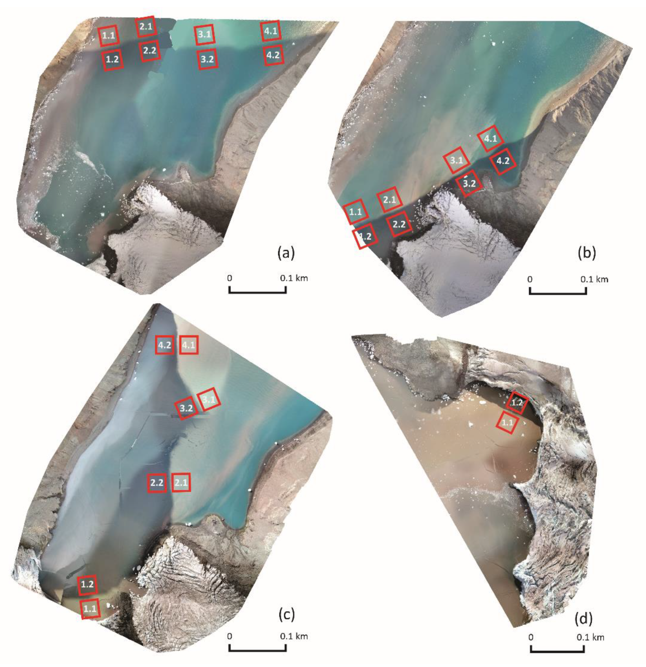
In this paper, the relationships between the spectral properties of meltwater in four spectral bands in the context of shaded and nonshaded areas were investigated. Four situations were considered: (1) shadow border extending far from the glacier front, clear water, no visible plumes, uniform, and low shortwave downward radiation (Figure 5a) (2) shadow border close to the glacier front and the shoreline, intensely saturated plumes of red color visible, slight but increasing shortwave downward radiation (Figure 5b); (3) shadow border along the cove, visible plumes of white and red color, changing and large radiation (Figure 5c); and (4) shadow border near the glacier front, shallow bottom, ice in the shaded area (Figure 5d). Sampling areas were separated on spectral maps from UAV and satellite images. This campaign examined four cases of reflectance maps obtained from UAV flights and four cases of reflectance maps from satellite images (Figure 5).
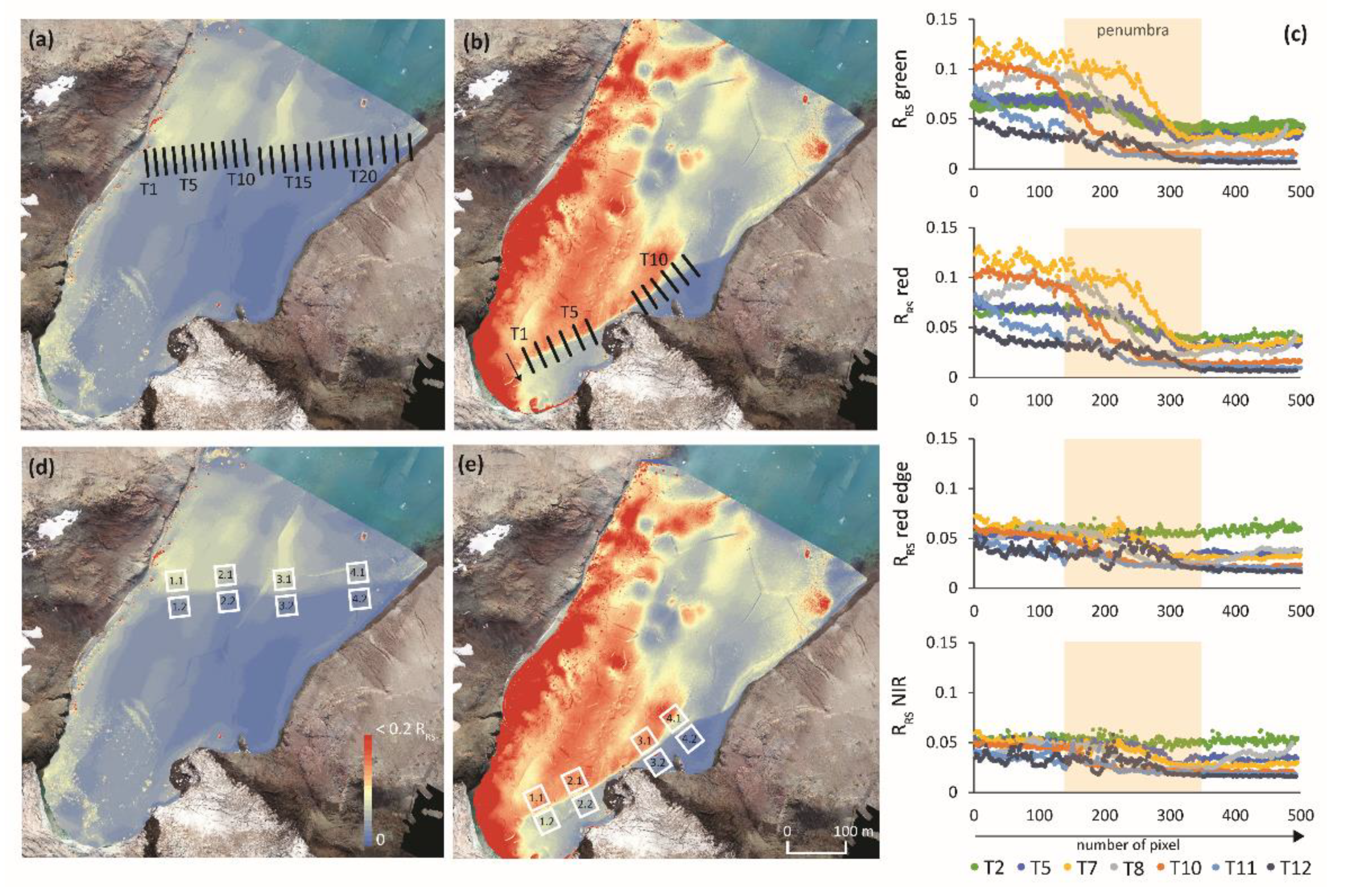
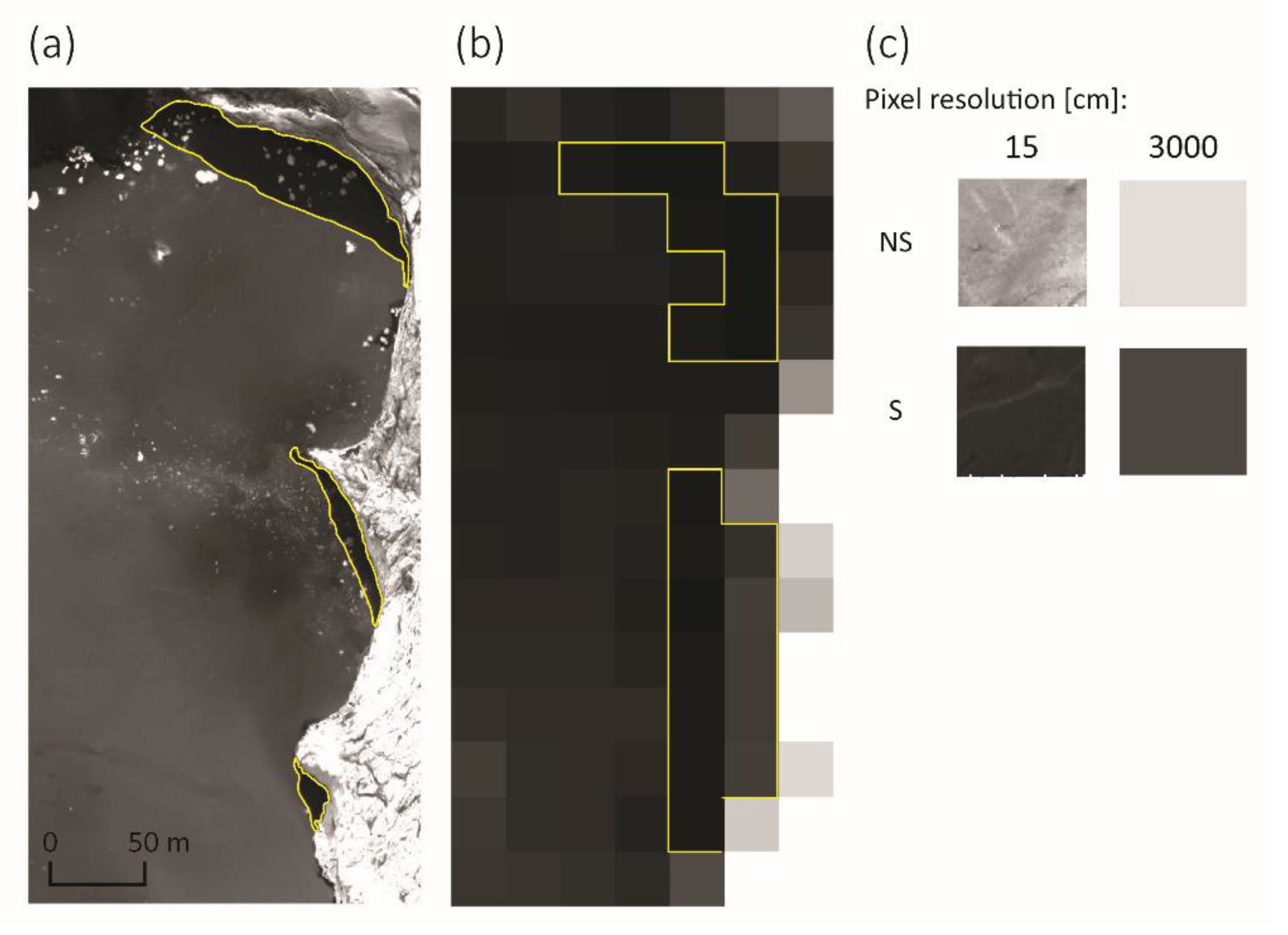
The first step was to construct transects perpendicular to the shadow border (Figure 6a,b). Then, transects with characteristics and visible umbra and solar and transition zones were selected (Figure 6c). The next step was to determine the sampling areas at the transect site in such a way that the designated sampling areas did not include the transition zone. For each case, four sampling areas were established, each consisting of two sub-areas (nonshadow and shadow) (Figure 6d,e). The side length of the sampling area was 30 m, which was related to the pixel resolution of Landsat 8 satellite images. To examine the phenomena of loss of accuracy and information (Figure 7a,b), analyses were carried out for the original pixel resolution (Table 1) and after aggregating pixels to 30 m (Figure 7c).
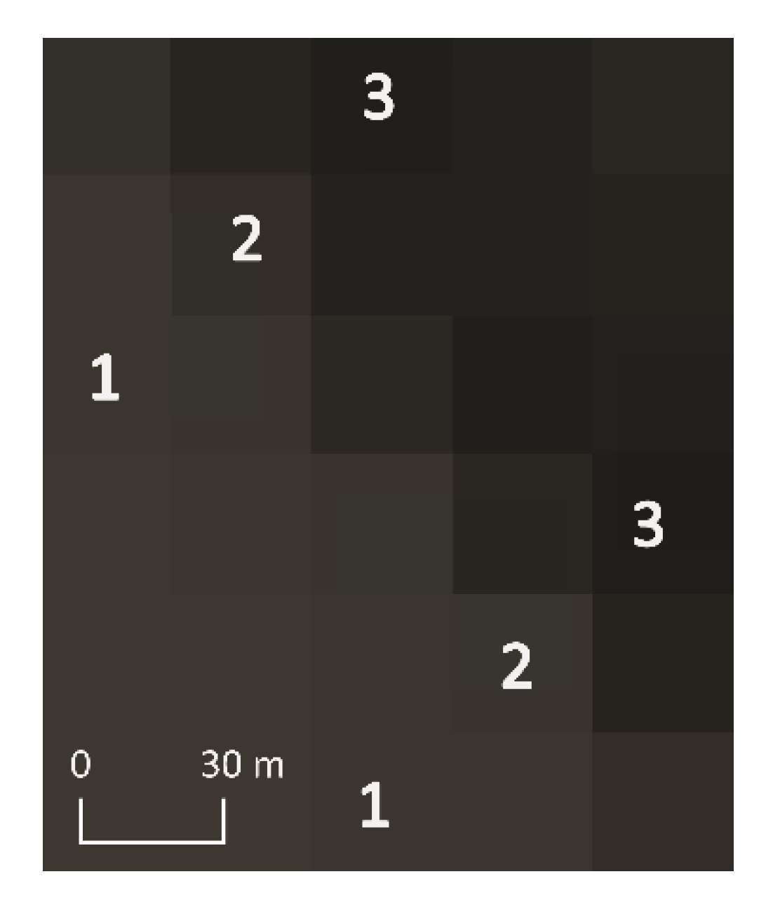
In contrast to UAV data, sampling areas for satellite images were determined in different ways. Due to the low pixel resolution (30 m) of Landsat 8 images and the invisible transition zones, perpendicular transects were not designed, as was done for UAV data. Despite this difference, three subareas—with shadows, without shadows and a third area where distinguishing between shadows and nonshadows was difficult—were assigned. Each subarea contained only one pixel in reference to pixel aggregation of UAV images. For each satellite image, two sampling areas with three subareas were determined. The zone between shadow and nonshadow areas was designated as an aid and was not considered in the analysis (Figure 8).
2.4. Shortwave Radiation Data Acquisition
Meteorological data for shortwave radiation were obtained from a meteorological station located in the vicinity of the Henryk Arctowski Polish Antarctic Station (Figure 1). The CNR4 net radiometer (Kipp & Zonen, Delft, The Netherlands) located at a height of 2 m a.s.l. in the tundra region recorded shortwave downward and upward radiation with a frequency of 1 s.
3. Results
3.1. Spatial and Temporal Distributions of Shadows
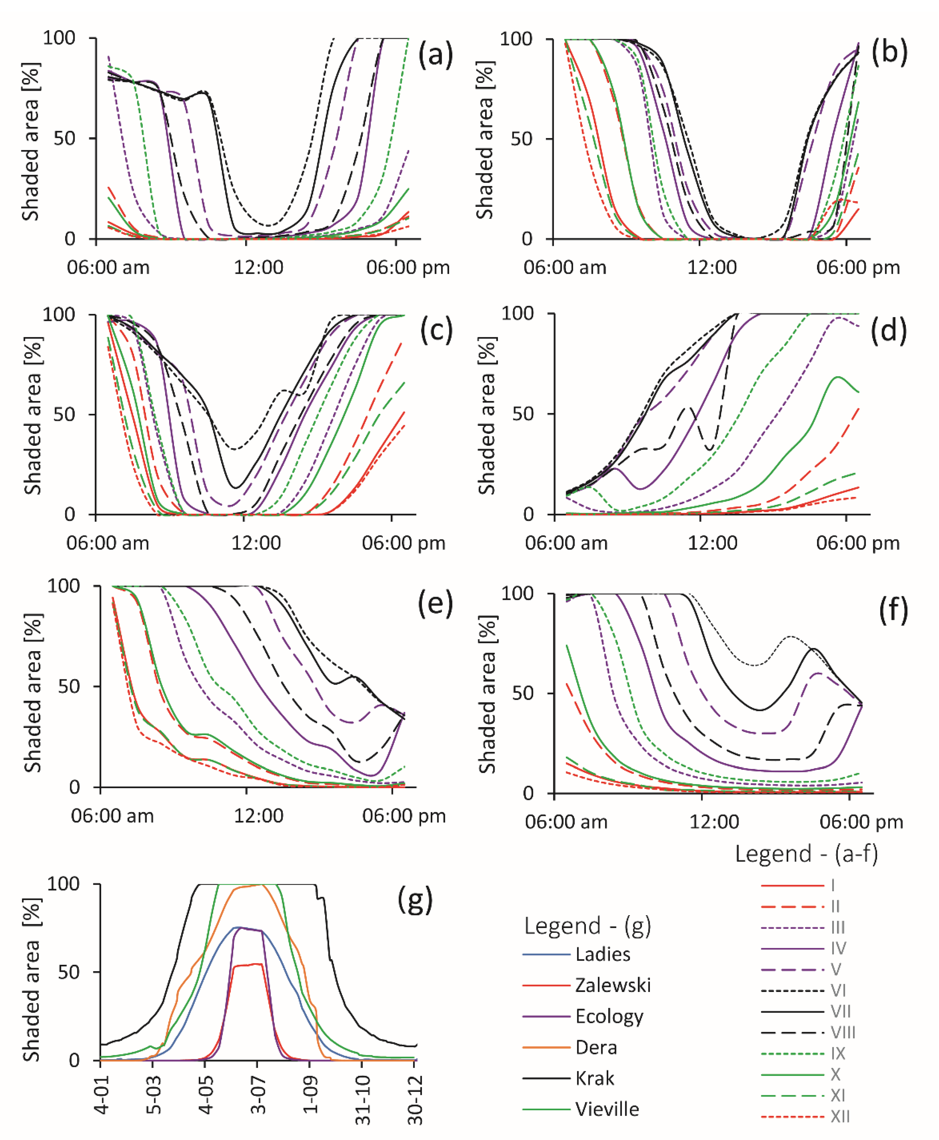
Figure 9 shows the variability in daily shadow distributions on the 15th day of each month. In the case of glaciers with northeastern exposure (Figure 9a,c), the maximum shadow reaches up to 100% of the area in the morning and afternoon and is minimal at mid-day. An important factor is the elevation of the glacier foreland and the indentation of the cove. The wide Suszczewski Cove (Figure 2a) surrounded by a relatively flat foreland has no shadow at noon in any month of the year (Figure 9a). A different situation is observed for glaciers whose valleys are long and deeply indented into surrounding steep slopes (Figure 2c). At noon during the summer, shadows are also not recorded in this case; however, in the winter months, the minimum shaded area can reach 40% of the bay (Figure 9c). The glacier with northwestern exposure and an open and shallow indented valley (Figure 2b) is the Ecology Glacier (Figure 9a), with the minimum shadow occurring an hour later (Figure 9b). This example represents a "U" type with maximum shadows in the morning and evening and a minimum at noon. A different shadow distribution at a glacier terminus with eastern exposure and a long and narrow cove is noted (Figure 2e). The maximum shadow occurs in the morning (with the shortening of the day, this moves to the noon hour), and the minimum is observed in the late afternoon and evening (Figure 9e). This example represents an “L” type with a maximum shadow in the morning and a minimum shadow in the evening. An icefall with a small, open bay with south and southwestern exposure (Figure 2d), in contrast to previous glaciers, is marked by the effect of "mirroring" with a minimum in the morning hours and a maximum in the late afternoon or evening (Figure 9d) and represents a “reflected L” type with a minimum shadow in the morning and a maximum shadow in the evening. Glaciers with S and SW exposures and open but shallow coves (Figure 2f) are heavily shaded in the morning hours and at noon, and the minimum shadow occurs in the late afternoon hours (Figure 9f). This glacier represents a mixed type, combining type “U” with “L”.
Figure 9g presents the percentage of shadows on the coves at the time the images were recorded by the satellite sensor on the following days of flight. The largest shadow areas occur from late fall to early winter (May–July), which is not a problem because the satellite sensor does not register images from mid-May to mid-August. In late spring and early summer (November-February), the shadow is small or absent in most of the analyzed cases. The exception is Lussich Cove near Krak Glacier, where the shadow occurs throughout the year and the minimum shadow area in November–February covers 10% of the cove.
3.2. Spectral Characteristics of the Sampling Area on UAV Multispectral Imagery
3.2.1. Shortwave Radiation Data
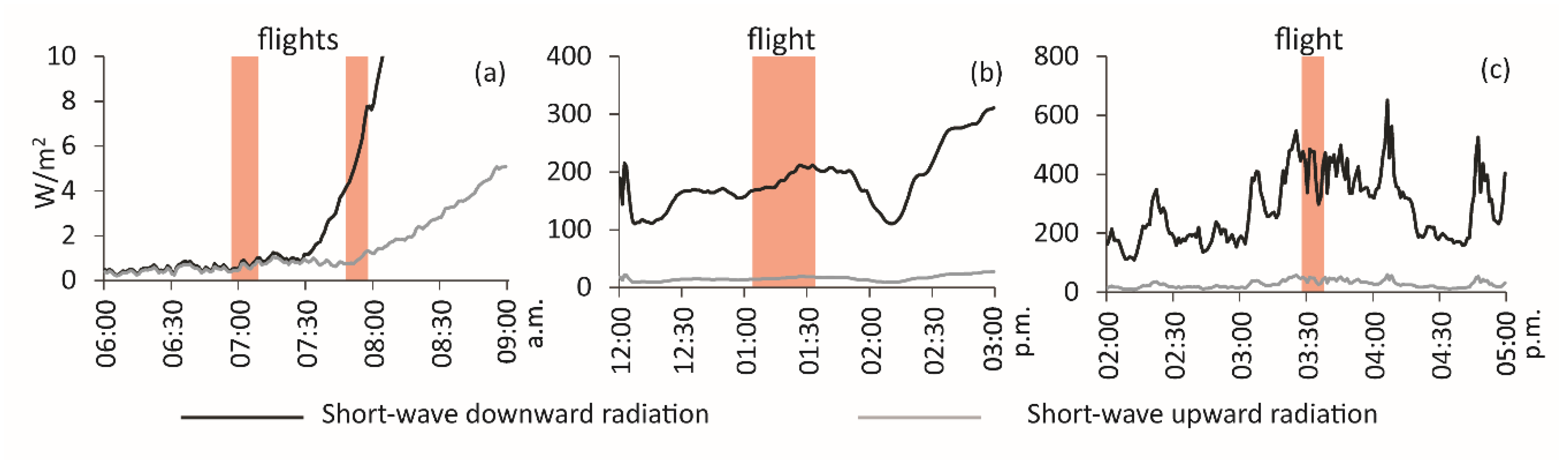
The amount of shortwave solar radiation depends on many factors, such as atmospheric attenuation (scattering and absorption) and Earth geometry [44]. On a local scale, the most important factor modifying the distribution of radiation is the terrain (exposure and slope). For these measurements, the radiation intensity was measured at a distance of 7 km from the sampling area; however, general conclusions can be drawn about the radiation situation on a given measurement day.
Three measurement days were analyzed, during which a total of four flights were carried out over the unnamed cove at Zalewski Glacier and Lussich Cove near Krak Glacier. The analysis involved the shortwave radiation recorded only during the flight time of the drone. During the first UAV flight on January 31st (Case Zalewski Glacier 1), both downward and upward radiation remained low. During the second flight on the same day, downward radiation dynamically increased, whereas upward radiation did not change (Figure 10a). On March 9th (Case Zalewski Glacier 2), downward radiation changed dynamically during the flight (Figure 10b). On March 5th (Case Krak Glacier 1), downward radiation was significantly higher (by almost 180 W/m2), but it did not change dynamically during the flight (Figure 10c).
3.2.2. Spectral Characteristic for Investigated Cases
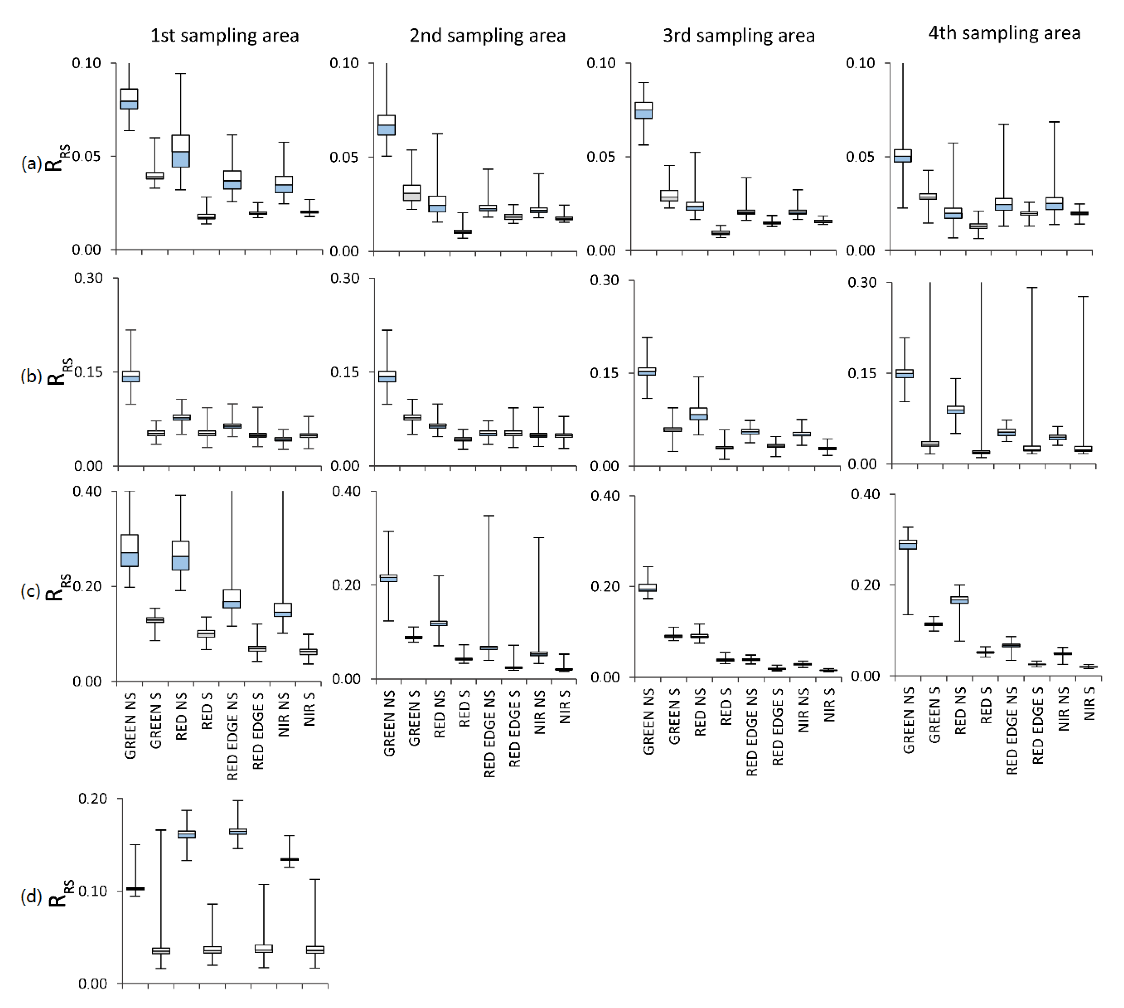
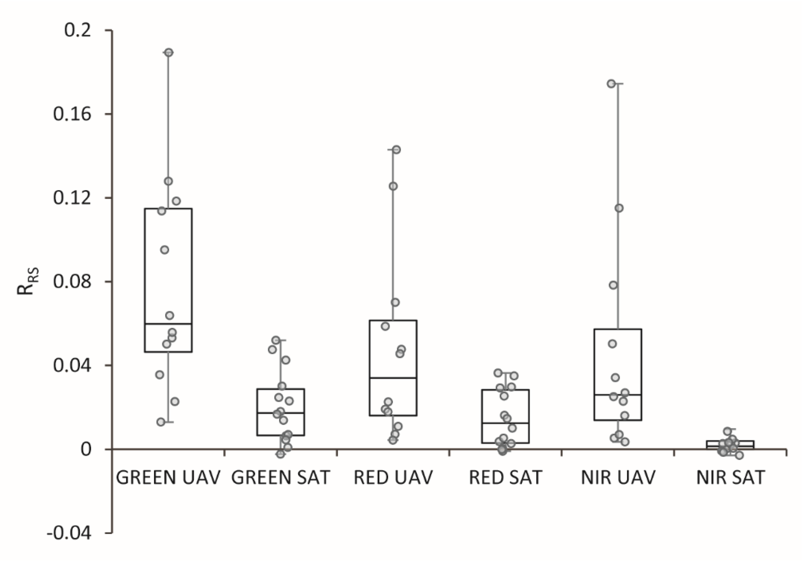
The largest difference in the range of values occurred in the fourth sampling area in the green spectral band (0.1 RRS) for the first case (Figure 11a, Figure A1), while the smallest difference was found in the second sampling area in the green spectral band (0.004 RRS). In case 2 (Figure 11b, Figure A2), the largest difference was observed in the fourth sampling area in the red edge (0.1 RRS), and the smallest in the first area in the red spectral band (0.007 RRS). In the second and third sampling areas in the red spectral band, the range in the shaded area was greater than that in the sunlit area (–0.005 RRS and –0.03 RRS, respectively). In case 3 (Figure 11c, Figure A3), the largest difference in the range of values was 0.028 RRS in red edge in the first sampling area and the smallest 0.007 RRS in the red edge in the third sampling area. In the Krak 1 case (Figure 11d, Figure A4), the highest difference was obtained in the red edge (0.13 RRS), and the smallest in the green spectral band (0.066 RRS).
The largest difference in medians between the shaded and nonshaded areas for all cases was recorded in the Zalewski 3 case (Figure 11c) in the green spectral band in the 4th sampling area and amounted to 0.178 RRS, and the smallest 0.0008 RRS in the Zalewski 2 (Figure 11b) case in the NIR in the fourth sampling area.
The greatest flattening of extreme values occurred in the Zalewski 3 case in the first sampling area in the red edge spectral band and amounted to 0.350 RRS, and the smallest in the Zalewski 1 case in the red edge spectral band. It is worth adding that in case Zalewski 2 in case 2 in the red edge spectral band, in case 4 in all bands and in case Krak 1 in the green spectral band, the maximum value in the shaded area was higher than in the nonshaded area. The results of the statistical tests are presented in Table A1 and more details are provided in Table A2.
3.2.3. Spectral Characteristics of Aggregated Pixels of UAV Images and Pixels of Satellite Imagery
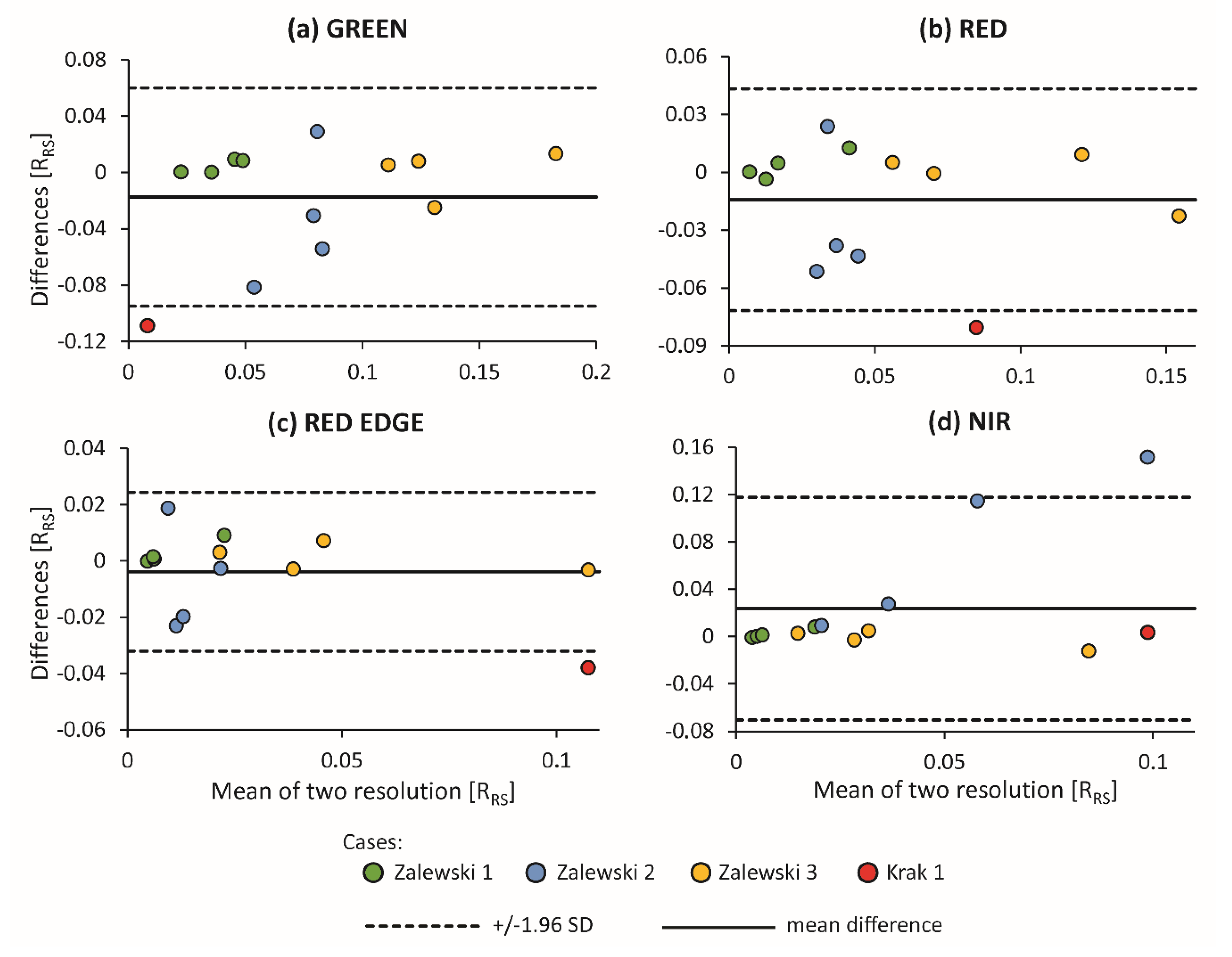
To analyze the loss of information in the spectrum that occurs with increasing spatial resolution of a pixel, aggregation of pixels with the original resolution of 15 cm to 30 m was performed. We compared the shift in reflection occurring between the shaded and nonshaded areas for the same sampling areas at two resolutions of 15 cm and 30 m using the Bland–Altman plot (Figure 12). In the 15 cm resolution, the average of all values from the 30 m area was used. The aggregation process up to a resolution of 30 m was done in ArcGIS software. The average reflection shifts for aggregated pixels (30 m) were lower than the reference values (15 cm). For the green spectral band, this difference is −0.01736 RRS, red −0.0142 RRS, and red edge −0.00383 RRS. Only in NIRs is this difference positive and amounts to 0.0236 RRS. The narrowest limits of agreement were observed in the red edge spectral band, and the widest limits were observed in the NIR band. However, the single outliers have the greatest impact on the limit agreement (for instance Krak 1 in the green and red spectral bands and Zalewski 2 in NIR) while the most points oscillate around zero. Zalewski 1 shows the most clustered values with the mean difference of measurements close to zero (green dots). Values for Zalewski 2 are different in relation to the Y axis blue dots, while the differences of shifts for Zalewski 3 oscillate approximately 0, but they are scattered with respect to the X axis (yellow dots). The difference in shifts for Krak only in the NIR is within the limits of agreement (red dots).
A comparative analysis between the UAV and satellite images is presented on the boxplot (Figure 13). It shows the differences in reflection shifts in individual spectral bands between the shaded and nonshaded areas obtained in UAV images with an aggregated resolution of up to 30 m and in satellite imagery. With regard to the lack of red edge spectral band in the spectrum recorded by Landsat, that spectral band was omitted from this analysis. Values recorded on satellite imagery are apparently lower than values on UAV images, which also makes shifts in reflection values between shaded and nonshaded areas are lower. In each case, the spectral band with shifts close to zero occurred, whereas in the NIR region, the reflectance value in the shaded area surpassed that in nonshaded area. The shifts of the values in the satellite images are 0.05 RRS smaller on average in the green spectral band, 0.03 RRS in the red spectral band and 0.04 RRS in the NIR than those obtained in the UAV images. The median difference in the green was 0.042 RRS, in the red 0.022 RRS, and 0.026 RRS in the NIR.
4. Discussion
The shadow distributions on the glacier coves during the Landsat 8 satellite passages over King George Island were analyzed. Although the number of flights was chosen to minimize the impact of the low angle of sunlight, shadows may occur all year in polar regions. An example is Lussich Cove by Krak Glacier. Its surface is shaded by a nearby hill, glacier fronts, or an ice dome, especially in spring or autumn. In the fall and spring, the coves are shaded from 20 to 100% (except for Zalewski Glaciers and Ecology Glacier). This makes problems for satellite observations of increasingly common mid-season thaws and winter rainfall, which are observed in both the Arctic [45] and Antarctic areas [46].
The hourly distribution of the shadow on the 15th of each month indicates the differences resulting from exposure, as well as the morphology of the glacier foreland or valley, which can be useful in planning UAV missions over water areas to provide appropriate conditions [47]. Three typical daily shadow distributions were identified. The first distribution is called the "U" type and is characteristic of coves with NE and NW exposures. The shadow minimum at noon eliminates the impact of high relief or rich bottom vegetation during mid-day flights [48]. The "L" distribution is the second type, characteristic of glaciers with W/NW exposures, and it features a minimum in the late afternoon/evening hours. The third type, called "the reflected L" distribution, is characteristic of glaciers with SE exposure with a minimum in the early morning hours. Flights in the early morning and late evening are suitable for "L" and "reflected L" types and minimize the glare effect [48].
Four scenarios (Figure 5) were analyzed to trace the spectral signature of glacial meltwater near glacier coves in shaded and nonshaded areas. The advantage of the conducted analysis is the possibility of tracing the spectral characteristics in spatial terms, enabling the determination of key concern in the creation of algorithms for detection but more for shadow compensation.
In the existing algorithms dealing with shadows within water bodies it is required that the water be homogeneous [31]; however, even in the case of pure water in the area with topographic shadows, the reflection in the entire shadow area is not uniformly reduced. It can be assumed that the occurrence of ’strong shadow and weak shadow’ also applies to water areas [48], which in this case is enhanced by low values of shortwave downward radiation and a small supply of solar energy both in the sunny area and in the shade. This is characterized by the fact that in the area of the cove furthest from the shadow-casting obstacle, the difference between the amount of radiation reflected in the nonshaded and shaded parts is greater than in the shallower area near this obstacle. In addition, this dependence also determines the amount of this radiation in spectral bands; the longer the electromagnetic wave is, the smaller this difference. Far from the obstacle within shadow in the green spectral band, the reflection is 50% less, and near the obstacle, it is 43% less. In NIR, these values are 42% and 21%, respectively. This relationship could also be seen from the diminishing median difference between nonshaded and shaded areas when approaching the obstacle. The uniform surface of the water and the absence of ice phenomena caused the ranges of values and maximum values in nonshaded areas in all spectral bands and all sampling areas to be greater than those in shaded areas. Despite the strong and weak shadow effect, pure homogeneous water allows to obtain the reflection coefficient of water in the shadow proportional to the reflection of pure water, and this relationship is useful for building algorithms [33].
Heavily turbid waters pose a major challenge for the OCR, due to the complex model of incident light scattering by suspended particulate matter, and therefore the attenuation of light within the water column dependent on water constituents, i.e., phytoplankton, SSC, colored dissolved organic matter [49]. It was shown in these studies that in the case of waters highly saturated with sediment, there are no spatial dependencies, and the spectral characteristics of the shadow depend on the type of sediment. In the case of saturation of the surface water layer with red-colored particles, previous studies have shown that it strongly correlates with the red, NIR, and short-wave infrared spectral bands depending on the concentration of SSC [50,51]. The white sediment, on the other hand, correlates more strongly with shorter electromagnetic waves [52]. In the green and red edge spectral bands, the amount of reflected radiation decreased by approximately 40%–50% in all sampling areas. However, in the red and NIR spectral bands, the differences in radiation reflection are small and amount to approximately 6% to 15% for the red spectral band and from 3% to 13% for the NIR. In addition, the shaded area is closer to the glacier, which means that it may be more saturated with SSC. The proximity of the glacier termini and shoreline as well as the presence of ice could have made the range of values in some sampling areas greater in shaded areas than in nonshaded areas, and the maximum values in shadow areas were greater than those in nonshadow areas. This indicates that sediment can disrupt the spectral reflectance curves of water and shadows [33]. If there was heterogeneous white and red sediment, the reflection signal in the entire shaded area, regardless of the spectral band, was lower by approximately 50%–60%. In the area closest to the glacier, where the water was saturated with heterogeneous sediment, the range of values was the widest, and it was the narrowest in the middle of the cove. The largest difference in medians was recorded in the area closest to the glacier, and the smallest difference was recorded in the middle of the cove. The difference in the maximum values between nonshadow and shadow areas was also the largest closest to glaciers. This situation could be influenced by the high position of the sun [53], but also by dynamically changing lighting (Figure 10).
The impact of spatial resolution on the spectral characteristics of shaded and nonshaded meltwaters was also analyzed. The reduction in the primary spatial resolution of UAV images reduces the accuracy and makes it impossible to find spatial characteristics, especially in small glacier coves. The result and the uncertainty of the results obtained strictly depend on the saturation of water with particles, but also on the amount of radiation. The value of the differences will be close to zero when the water is uniform and clean and the radiation is uniform (Zalewski 1). When the water is saturated with sediment and the shadow border runs close to the glacier’s front line or close to the shoreline and the value of the incident radiation will be slight, the differences in shifts between the resolutions will vary by over 100% of the reference value (Zalewski 2). A particular example is when ice is present in the shaded area, causing an overestimation when the resolution is reduced.
Similar differences in values were obtained during comparative analysis of shifts between shaded and nonshaded areas in UAV (30 m) images and satellite images. The lower reflectance values recorded by the satellite sensor may depend on the transparency of the atmosphere, aerosols, the atmospheric correction used and the technical specificity of the sensor itself.
The phenomenon of shadow influence on highly turbid waters requires further research, especially in the context of the heterogeneity of sediment and saturation, ice phenomena, and the spectral characteristics of shallow waters with different ground types and variable depths. Algorithms for the detection and compensation of shadows in polar regions may need to validate the physicochemical parameters of water that affect optical properties [54] and will also need to adjust for seasonal variability, such as mid-winter thaw, release of meltwater in the summer season, and bloom events [3]. This fact in turn suggests that the de-shadowing algorithms in polar regions should be adapted to the prevailing conditions. Although shadows in cold regions are a large-scale phenomenon, the creation of such algorithms is extremely important, especially in the case of ocean color radiometry, which is based on low reflectance values, and even a slight variation in these values can perturb the analysis.
Currently, existing algorithms are often flawed in water areas in general or in shallow or turbid waters. The main problem with the frequently used threshold method is that it is difficult to distinguish between real pixels in shadow and nonshadow areas, such as water, due to the phenomenon of pixel similarity [15]. In the case of the histogram method, it would be difficult to distinguish the reflection from highly turbid, shaded, and nonshaded water. Numerous algorithms use the method of neighboring areas, but they require homogeneous conditions throughout the analyzed area [31,55]. The linear relationship between shadow and nonshadow areas is also increasingly used, however, the main problem with these algorithms is that they have lost local variability for each class, due to being implemented globally [55].
5. Conclusions
In this paper, we fill the knowledge gap in the characteristics of water shadows in cold regions and provide a specific supplement to the recommendations made by Shahtahmassebi et al. [15]. Creating an algorithm for topographic shadow correction and building techniques that treat the shadow surface as a heterogeneous structure are necessary, as well as developing and presenting methods in forms that allow the user to apply them in a specific region [15].
Our findings may be summarized by the following conclusions:
- Shadows significantly affect the spectral properties of meltwater, reducing the amount of reflected radiation. Ocean color radiometry, which is based on very low radiation values, is relevant because it can cause significant differences.
- UAV images enable the determination of spatial changes in the spectral characteristics of shaded water:
- (a)
- A uniform surface of shaded water (low turbidity and no ice phenomena) tends to change its spectral properties during the approach to an obstacle casting a shadow.
- (b)
- With highly turbid, shallow water and ice phenomena, spatial tendency does not occur. In this case, the spectral signature depends on the sediment type and the saturation of the SSC surface water layer.
- (c)
- Within highly suspended water, the difference in reflection in the shaded and nonshaded areas will be smaller.
- (d)
- Ice and a shallow bottom in the immediate vicinity of the glacier front in the shaded area may disturb the analysis.
- (e)
- The difference between the amount of radiation reflected in the shaded and nonshaded areas depends on the amount of shortwave downward radiation (time of the day).
- Pixel aggregation of uniform areas causes the loss of detailed information, while pixel aggregation of nonuniform, shallow areas with ice phenomena causes changes and the loss of original information.
- The reflection in the satellite imagery is much smaller in both the nonshaded and shaded areas than in the UAV images. In NIRs, shifts between shadow and nonshadow areas are often close to 0 or even negative.
- The characteristics of the spectral bands in the shaded area are as follows:
- (a)
- The green spectral band has the highest contrast in the amount of reflected radiation between NS and S, but due to its high sensitivity, the analysis can be overestimated.
- (b)
- In the RE and NIR, the values in shaded areas are uniform and without contrast, which makes it impossible to obtain primary information about the spectral characteristics of water.
Author Contributions
Conceptualization, K.A.W.-D. and R.J.B.; methodology, K.A.W.-D.; investigation, K.A.W.-D.; data curation, K.A.W.-D. and R.J.B.; writing original draft preparation, K.A.W.-D.; resources, K.A.W.-D.; supervision, project administration and funding acquisition R.J.B. All authors have read and agreed to the published version of the manuscript.
Funding
The National Science Centre, Poland, grant no. 2017/25/B/ST10/02092 ‘Quantitative Assessment of Sediment Transport from Glaciers of South Shetland Islands On The Basis Of Selected Remote Sensing Methods’ supported this work.
Institutional Review Board Statement
Not applicable.
Informed Consent Statement
Not applicable.
Data Availability Statement
The data presented in this study are available on request from the corresponding author.
Acknowledgments
We appreciate the support provided by the Arctowski Polish Antarctic Station. We are particularly grateful to Maria Osińska, Marek Figielski and Tomasz Kurczaba for their help in collecting data. Special thanks to ESRI for providing the ArcGIS Advanced 10.6 to Kornelia Wójcik, which helped complete most analyses.
Conflicts of Interest
The authors declare no conflict of interest.
Appendix A
Statistical analysis was used to determine the statistical significance between the reflectance values of shaded and nonshaded areas on UAV images with 15 cm resolution. To achieve the set goal, the Kolomogorov-Smirnov test for normality of the distribution was initially performed, and the nonparametric Mann-Whitney U test to compare two independent samples at significance level α = 0.05 was then implemented.

Table A1.
Results of the nonparametric Mann-Whitney U test (+ statistically significant, − statistically insignificant).
Table A1.
Results of the nonparametric Mann-Whitney U test (+ statistically significant, − statistically insignificant).
| Zalewski 1 | ||||||||||||||||||||||
| 1.1/1.2 | 2.1/2.2 | 3.1/3.2 | 4.1/4.2 | |||||||||||||||||||
| GR | RD | RG | NIR | GR | RD | RG | NIR | GR | RD | RG | NIR | GR | RD | RG | NIR | |||||||
| GR | + | + | + | + | ||||||||||||||||||
| RD | + | + | + | + | ||||||||||||||||||
| RG | + | + | + | + | ||||||||||||||||||
| NIR | + | + | + | + | ||||||||||||||||||
| Zalewski 2 | ||||||||||||||||||||||
| GR | + | + | + | + | ||||||||||||||||||
| RD | + | + | + | + | ||||||||||||||||||
| RG | + | - | + | + | ||||||||||||||||||
| NIR | + | + | + | + | ||||||||||||||||||
| Zalewski 3 | ||||||||||||||||||||||
| GR | + | + | + | + | ||||||||||||||||||
| RD | + | + | + | + | ||||||||||||||||||
| RG | + | + | + | + | ||||||||||||||||||
| NIR | + | + | + | + | ||||||||||||||||||
| Krak 1 | ||||||||||||||||||||||
| GR | + | |||||||||||||||||||||
| RD | + | |||||||||||||||||||||
| RG | + | |||||||||||||||||||||
| NIR | + | |||||||||||||||||||||
Table A2.
Spectral characteristics of cases.
| Zalewski 1 | ||||||||||||||||
| 1.1/1.2 | 2.1/2.2 | 3.1/3.2 | 4.1/4.2 | |||||||||||||
| Differences in: * | GR | RD | RG | NIR | GR | RD | RG | NIR | GR | RD | RG | NIR | GR | RD | RG | NIR |
| range | 0.032 | 0.048 | 0.028 | 0.0237 | 0.004 | 0.012 | 0.005 | 0.008 | 0.0105 | 0.030 | 0.017 | 0.0113 | 0.100 | 0.036 | 0.042 | 0.044 |
| median | 0.041 | 0.035 | 0.018 | 0.015 | 0.036 | 0.014 | 0.005 | 0.004 | 0.047 | 0.014 | 0.006 | 0.005 | 0.022 | 0.007 | 0.005 | 0.005 |
| max. values | 0.063 | 0.066 | 0.036 | 0.031 | 0.032 | 0.020 | 0.008 | 0.010 | 0.044 | 0.039 | 0.020 | 0.014 | 0.108 | 0.036 | 0.042 | 0.044 |
| Zalewski 2 | ||||||||||||||||
| range * | −0.006 | 0.008 | 0.025 | 0.008 | 0.066 | −0.025 | 0.025 | 0.012 | 0.005 | −0.005 | 0.023 | 0.006 | 0.014 | 0.004 | 0.106 | 0.015 |
| median * | 0.070 | 0.004 | 0.029 | 0.004 | 0.079 | 0.003 | 0.034 | 0.003 | 0.070 | 0.004 | 0.029 | 0.004 | 0.060 | 0.008 | 0.014 | 0.001 |
| max. values * | 0.100 | 0.087 | 0.027 | 0.023 | 0.110 | 0.041 | −0.021 | 0.015 | 0.114 | 0.086 | 0.026 | 0.031 | −0.209 | −0.165 | −0.220 | −0.215 |
| Zalewski 3 | ||||||||||||||||
| range * | 0.135 | 0.132 | 0.276 | 0.243 | 0.165 | 0.112 | 0.121 | 0.082 | 0.041 | 0.018 | 0.007 | 0.007 | 0.161 | 0.101 | 0.039 | 0.028 |
| median * | 0.141 | 0.162 | 0.099 | 0.083 | 0.128 | 0.076 | 0.042 | 0.033 | 0.105 | 0.053 | 0.020 | 0.014 | 0.178 | 0.116 | 0.042 | 0.029 |
| max. values * | 0.247 | 0.256 | 0.350 | 0.308 | 0.211 | 0.150 | 0.142 | 0.099 | 0.134 | 0.063 | 0.022 | 0.016 | 0.197 | 0.136 | 0.054 | 0.037 |
| Krak 1 | ||||||||||||||||
| range * | −0.122 | −0.066 | −0.040 | −0.016 | ||||||||||||
| median * | 0.066 | 0.096 | 0.125 | 0.122 | ||||||||||||
| max. values * | −0.042 | 0.048 | 0.094 | 0.111 | ||||||||||||
* with an assumption: NS − S.
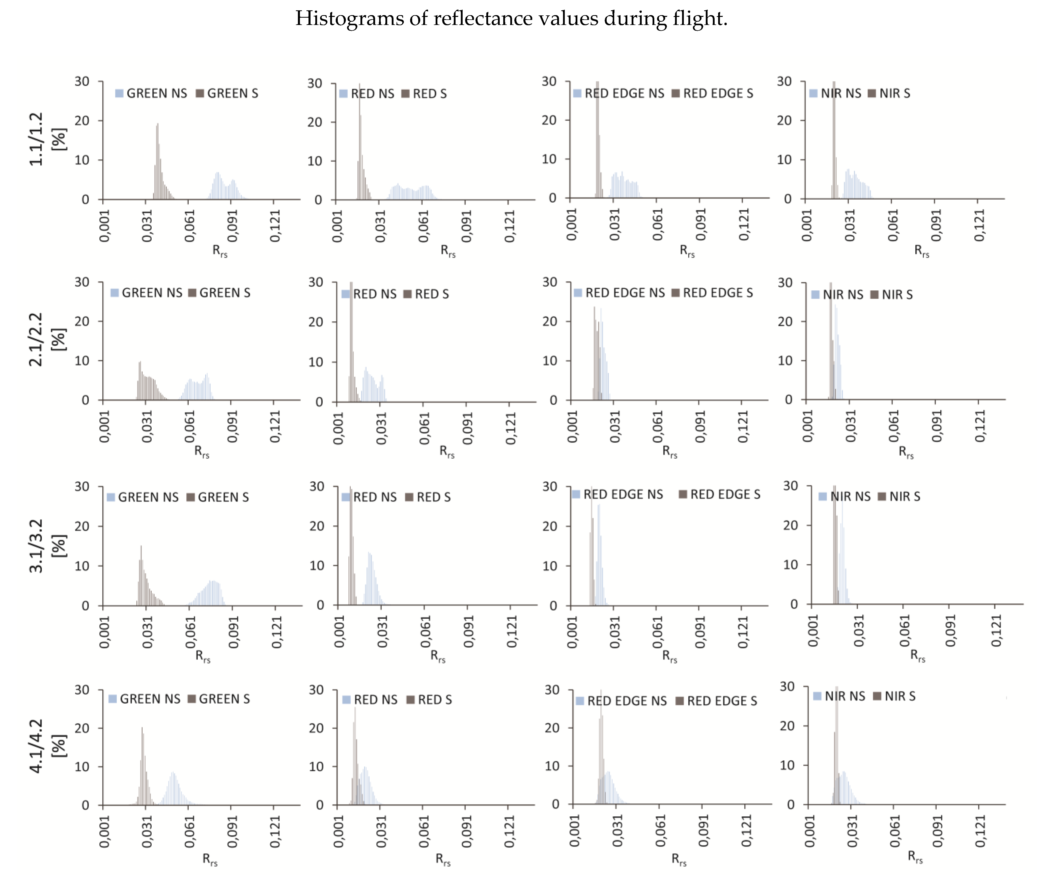
Figure A1.
Histograms of reflectance values for case Zalewski 1.

Figure A2.
Histograms of reflectance values for case Zalewski 2.

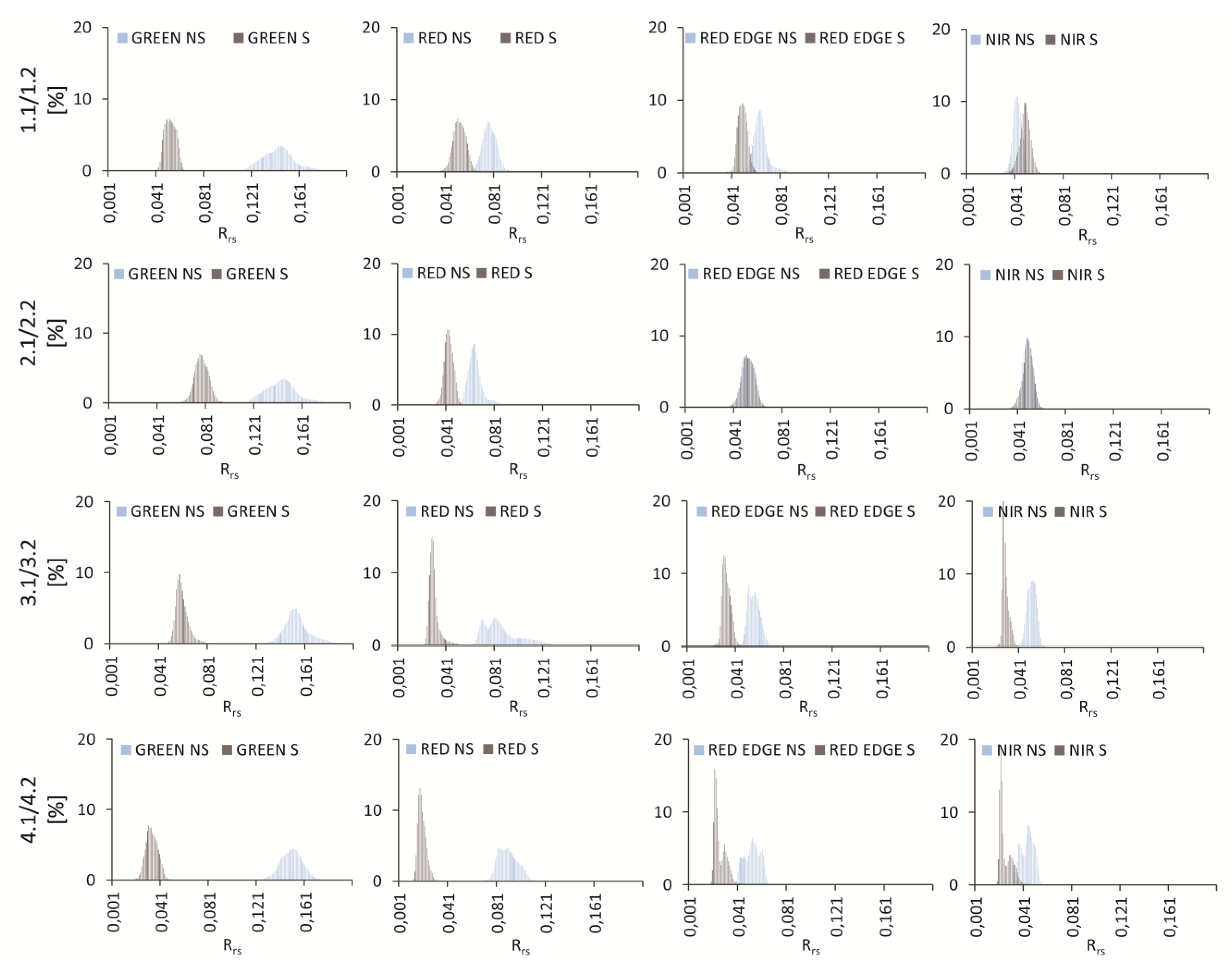
Figure A3.
Histograms of reflectance values for case Zalewski 3.

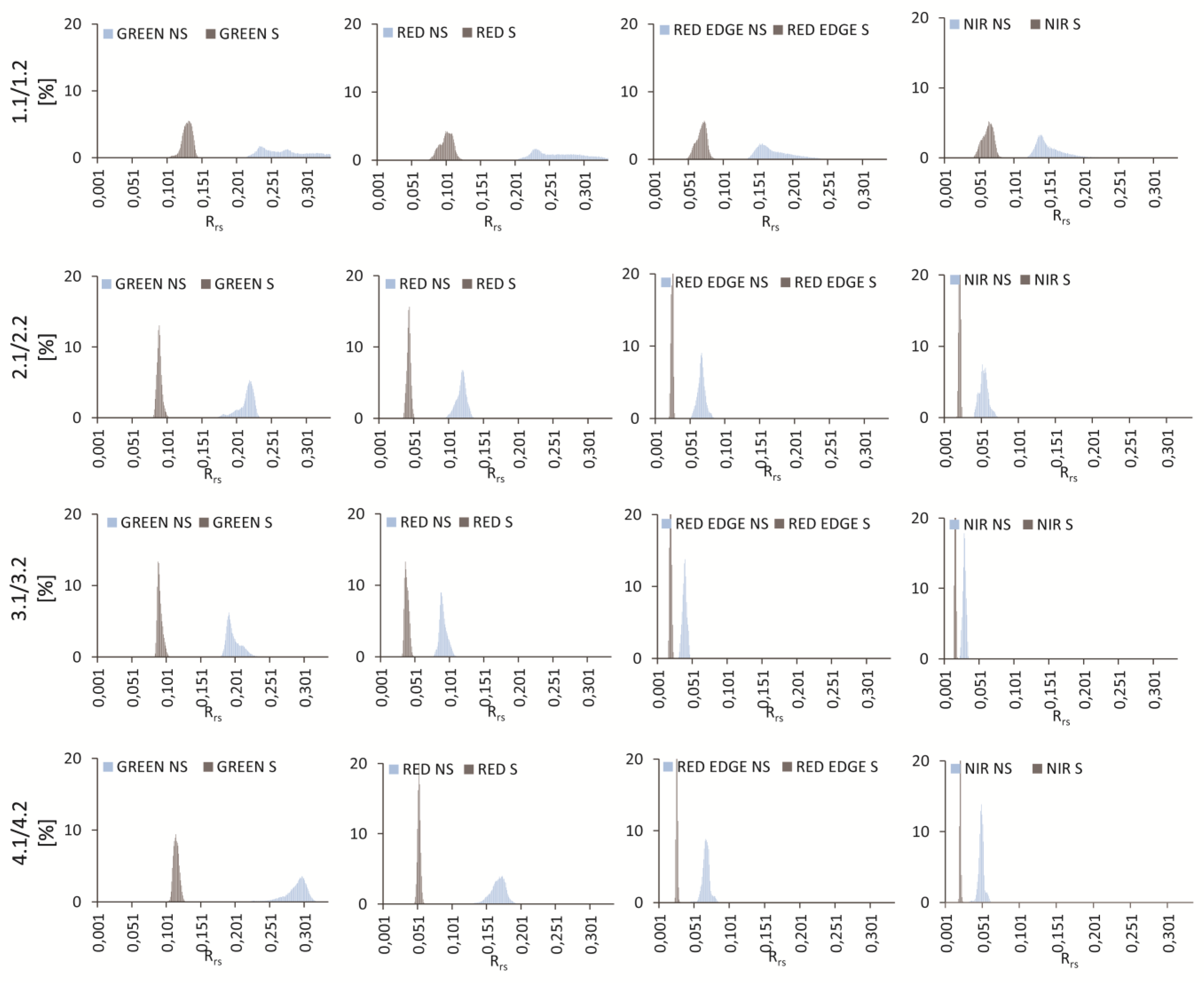
Figure A4.
Histograms of reflectance values for case Krak 1.

References
- Frederikse, T.; Landerer, F.; Caron, L.; Adhikari, S.; Parkes, D.; Humphrey, V.; Dangendorf, S.; Hogarth, P.; Zanna, L.; Cheng, L.; et al. The causes of sea-level rise since 1900. Nature 2020, 584, 393–397. [Google Scholar] [CrossRef] [PubMed]
- Aracena, C.; González, H.E.; Garcés-Vargas, J.; Lange, C.B.; Pantoja, S.; Muñoz, F.; Teca, E.; Tejos, E. Influence of summer conditions on surface water properties and phytoplankton productivity in embayments of the South Shetland Islands. Polar Biol. 2018, 41, 2135–2155. [Google Scholar] [CrossRef]
- Meredith, M.P.; Falk, U.; Bers, A.V.; Mackensen, A.; Schloss, I.R.; Barlett, E.R.; Jerosch, K.; Busso, A.S.; Abele, D. Anatomy of a glacial meltwater discharge event in an Antarctic cove. Philos. Trans. R. Soc. A Math. Phys. Eng. Sci. 2018, 376, 20170163. [Google Scholar] [CrossRef]
- Carroll, D.; Sutherland, D.A.; Hudson, B.; Moon, T.; Catania, G.A.; Shroyer, E.L.; Nash, J.D.; Bartholomaus, T.C.; Felikson, D.; Stearns, L.A.; et al. The impact of glacier geometry on meltwater plume structure and submarine melt in Greenland fjords. Geophys. Res. Lett. 2016, 43, 9739–9748. [Google Scholar] [CrossRef] [Green Version]
- Vernet, M.; Martinson, D.; Iannuzzi, R.; Stammerjohn, S.; Kozlowski, W.; Sines, K.; Smith, R.; Garibotti, I. Primary production within the sea-ice zone west of the Antarctic Peninsula: I—Sea ice, summer mixed layer, and irradiance. Deep Sea Res. Part II Top. Stud. Oceanogr. 2008, 55, 2068–2085. [Google Scholar] [CrossRef]
- Pan, B.J.; Vernet, M.; Reynolds, R.A.; Mitchell, B.G. The optical and biological properties of glacial meltwater in an Antarctic fjord. PLoS ONE 2019, 14, e0211107. [Google Scholar] [CrossRef] [Green Version]
- Straneo, F.; Cenedese, C. The dynamics of Greenland’s glacial fjords and their role in climate. Annu. Rev. Mar. Sci. 2015, 7, 89–112. [Google Scholar] [CrossRef]
- Fegel, T.S.; Baron, J.S.; Fountain, A.G.; Johnson, G.F.; Hall, E.K. The differing biogeochemical and microbial signatures of glaciers and rock glaciers. J. Geophys. Res. Biogeosciences 2016, 121, 919–932. [Google Scholar] [CrossRef] [Green Version]
- How, P.; Benn, D.I.; Hulton, N.R.; Hubbard, B.; Luckman, A.; Sevestre, H.; Van Pelt, W.; Lindbäck, K.; Kohler, J.; Boot, W. Rapidly changing subglacial hydrological pathways at a tidewater glacier revealed through simultaneous observations of water pressure, supraglacial lakes, meltwater plumes and surface velocities. Cryosphere 2017, 11, 2691–2710. [Google Scholar] [CrossRef] [Green Version]
- McGrath, D.; Steffen, K.; Overeem, I.; Mernild, S.H.; Hasholt, B.; Van Den Broeke, M. Sediment plumes as a proxy for local ice-sheet runoff in Kangerlussuaq Fjord, West Greenland. J. Glaciol. 2010, 56, 813–821. [Google Scholar] [CrossRef] [Green Version]
- Dierssen, H.M.; Smith, R.C.; Vernet, M. Glacial meltwater dynamics in coastal waters west of the Antarctic peninsula. Proc. Natl. Acad. Sci. USA 2002, 99, 1790–1795. [Google Scholar] [CrossRef] [PubMed] [Green Version]
- Truffer, M.; Motyka, R.J. Where glaciers meet water: Subaqueous melt and its relevance to glaciers in various settings. Rev. Geophys. 2016, 54, 220–239. [Google Scholar] [CrossRef] [Green Version]
- Manfreda, S.; McCabe, M.F.; Miller, P.E.; Lucas, R.; Pajuelo Madrigal, V.; Mallinis, G.; Ben-Dor, E.; Helman, D.; Estes, L.; Ciraolo, G.; et al. On the use of unmanned aerial systems for environmental monitoring. Remote Sens. 2018, 10, 641. [Google Scholar] [CrossRef] [Green Version]
- Whitehead, K.; Hugenholtz, C.H.; Myshak, S. Remote sensing of the environment with small unmanned aircraft systems (UASs), part 2: Scientific and commercial applications. J. Unmanned Veh. Syst. 2014, 2, 86–102. [Google Scholar] [CrossRef] [Green Version]
- Shahtahmassebi, A.; Yang, N.; Wang, K.; Moore, N.; Shen, Z. Review of shadow detection and de-shadowing methods in remote sensing. Chin. Geogr. Sci. 2013, 23, 403–420. [Google Scholar] [CrossRef] [Green Version]
- Chen, Q.; Zhang, G.; Yang, X.; Li, S.; Li, Y.; Wang, H.H. Single image shadow detection and removal based on feature fusion and multiple dictionary learning. Multimed. Tools Appl. 2018, 77, 18601–18624. [Google Scholar] [CrossRef]
- Liasis, G.; Stavrou, S. Satellite images analysis for shadow detection and building height estimation. ISPRS J. Photogramm. Remote Sens. 2016, 119, 437–450. [Google Scholar] [CrossRef]
- Sarabandi, P.; Yamazaki, F.; Matsuoka, M.; Kiremidjian, A. Shadow detection and radiometric restoration in satellite high resolution images. IEEE Int. Geosci. Remote Sens. Symp. 2004, 6, 3744–3747. [Google Scholar] [CrossRef]
- Wang, Q.; Yan, L.; Yuan, Q.; Ma, Z. An automatic shadow detection method for VHR remote sensing orthoimagery. Remote Sens. 2017, 9, 469. [Google Scholar] [CrossRef] [Green Version]
- Wu, S.T.; Hsieh, Y.T.; Chen, C.T.; Chen, J.C. A Comparison of 4 shadow compensation techniques for land cover classification of shaded areas from high radiometric resolution aerial images. Can. J. Remote Sens. 2014, 40, 315–326. [Google Scholar] [CrossRef]
- Yamazaki, F.; Liu, W.; Takasaki, M. Characteristics of shadow and removal of its effects for remote sensing imagery. IEEE Int. Geosci. Remote Sens. Symp. 2009, 4, 426. [Google Scholar] [CrossRef]
- França, M.M.; Fernandes Filho, E.I.; Ferreira, W.P.; Lani, J.L.; Soares, V.P. Topographic shadow influence on optical image acquired by satellite in the southern hemisphere. Eng. Agric. 2018, 38, 728–740. [Google Scholar] [CrossRef]
- Movia, A.; Beinat, A.; Crosilla, F. Shadow detection and removal in RGB VHR images for land use unsupervised classification. ISPRS J. Photogramm. Remote Sens. 2016, 119, 485–495. [Google Scholar] [CrossRef]
- Arévalo, V.; González, J.; Ambrosio, G. Shadow detection in colour high-resolution satellite images. Int. J. Remote Sens. 2008, 29, 1945–1963. [Google Scholar] [CrossRef]
- Qiao, X.; Yuan, D.; Li, H. Urban shadow detection and classification using hyperspectral image. J. Indian Soc. Remote Sens. 2017, 45, 945–952. [Google Scholar] [CrossRef]
- Tatar, N.; Saadatseresht, M.; Arefi, H.; Hadavand, A. A robust object-based shadow detection method for cloud-free high resolution satellite images over urban areas and water bodies. Adv. Space Res. 2018, 61, 2787–2800. [Google Scholar] [CrossRef]
- Yang, J.; He, Y.; Caspersen, J. Fully constrained linear spectral unmixing based global shadow compensation for high resolution satellite imagery of urban areas. Int. J. Appl. Earth Obs. Geoinf. 2015, 38, 88–98. [Google Scholar] [CrossRef]
- Aboutalebi, M.; Torres-Rua, A.F.; Kustas, W.P.; Nieto, H.; Coopmans, C.; McKee, M. Assessment of different methods for shadow detection in high-resolution optical imagery and evaluation of shadow impact on calculation of NDVI, and evapotranspiration. Irrig. Sci. 2019, 37, 407–429. [Google Scholar] [CrossRef]
- Poblete, T.; Ortega-Farías, S.; Ryu, D. Automatic coregistration algorithm to remove canopy shaded pixels in UAV-borne thermal images to improve the estimation of crop water stress index of a drip-irrigated Cabernet Sauvignon vineyard. Sensors 2018, 18, 397. [Google Scholar] [CrossRef] [Green Version]
- Tarko, A.; De Bruin, S.; Bregt, A.K. Comparison of manual and automated shadow detection on satellite imagery for agricultural land delineation. Int. J. Appl. Earth Obs. Geoinf. 2018, 73, 493–502. [Google Scholar] [CrossRef]
- Amin, R.; Gould, R.; Hou, W.; Arnone, R.; Lee, Z. Optical algorithm for cloud shadow detection over water. IEEE Trans. Geosci. Remote Sens. 2012, 51, 732–741. [Google Scholar] [CrossRef]
- Mostafa, Y.; Abdelhafiz, A. Shadow identification in high resolution satellite images in the presence of water regions. Photogramm. Eng. Remote Sens. 2017, 83, 87–94. [Google Scholar] [CrossRef]
- Xie, H.; Luo, X.; Xu, X.; Tong, X.; Jin, Y.; Pan, H.; Zhou, B. New hyperspectral difference water index for the extraction of urban water bodies by the use of airborne hyperspectral images. J. Appl. Remote Sens. 2014, 8, 085098. [Google Scholar] [CrossRef] [Green Version]
- Zeng, C.; Richardson, M.; King, D.J. The impacts of environmental variables on water reflectance measured using a lightweight unmanned aerial vehicle (UAV)-based spectrometer system. Isprs J. Photogramm. Remote Sens. 2017, 130, 217–230. [Google Scholar] [CrossRef]
- Amin, R.; Zhou, J.; Gilerson, A.; Gross, B.; Moshary, F.; Ahmed, S. Novel optical techniques for detecting and classifying toxic dinoflagellate Karenia brevis blooms using satellite imagery. Opt. Express 2009, 17, 9126–9144. [Google Scholar] [CrossRef]
- Rückamp, M.; Braun, M.; Suckro, S.; Blindow, N. Observed glacial changes on the King George Island ice cap, Antarctica, in the last decade. Glob. Planet. Chang. 2011, 79, 99–109. [Google Scholar] [CrossRef]
- Wójcik, K.A.; Bialik, R.J.; Osińska, M.; Figielski, M. Investigation of Sediment-Rich Glacial Meltwater Plumes Using a High-Resolution Multispectral Sensor Mounted on an Unmanned Aerial Vehicle. Water 2019, 11, 2405. [Google Scholar] [CrossRef] [Green Version]
- Gindraux, S.; Boesch, R.; Farinotti, D. Accuracy assessment of digital surface models from unmanned aerial vehicles’ imagery on glaciers. Remote Sens. 2017, 9, 186. [Google Scholar] [CrossRef] [Green Version]
- Jaud, M.; Passot, S.; Le Bivic, R.; Delacourt, C.; Grandjean, P.; Le Dantec, N. Assessing the accuracy of high resolution digital surface models computed by PhotoScan® and MicMac® in sub-optimal survey conditions. Remote Sens. 2016, 8, 465. [Google Scholar] [CrossRef] [Green Version]
- Available online: https://desktop.arcgis.com/ (accessed on 22 December 2020).
- Novoa, S.; Doxaran, D.; Ody, A.; Vanhellemont, Q.; Lafon, V.; Lubac, B.; Gernez, P. Atmospheric corrections and multi-conditional algorithm for multi-sensor remote sensing of suspended particulate matter in low-to-high turbidity levels coastal waters. Remote Sens. 2017, 9, 61. [Google Scholar] [CrossRef] [Green Version]
- Zhang, Z.; He, G.; Wang, X. A practical DOS model-based atmospheric correction algorithm. Int. J. Remote Sens. 2010, 31, 2837–2852. [Google Scholar] [CrossRef]
- Mostafa, Y. A review on various shadow detection and compensation techniques in remote sensing images. Can. J. Remote Sens. 2017, 43, 545–562. [Google Scholar] [CrossRef]
- Montero, G.; Escobar, J.M.; Rodríguez, E.; Montenegro, R. Solar radiation and shadow modelling with adaptive triangular meshes. Sol. Energy 2009, 83, 998–1012. [Google Scholar] [CrossRef]
- Łupikasza, E.B.; Ignatiuk, D.; Grabiec, M.; Cielecka, K.; Laska, M.; Jania, J.A.; Luks, B.; Uszczyk, A.; Budzik, T. The Role of Winter Rain in the Glacial System on Svalbard. Water 2019, 11, 334. [Google Scholar] [CrossRef] [Green Version]
- Rachlewicz, G. Mid-winter thawing in the vicinity of Arctowski Station, King George Island. Pol. Polar Res. 1997, 18, 15–24. [Google Scholar]
- Gray, P.C.; Ridge, J.T.; Poulin, S.K.; Seymour, A.C.; Schwantes, A.M.; Swenson, J.J.; Johnston, D.W. Integrating drone imagery into high resolution satellite remote sensing assessments of estuarine environments. Remote Sens. 2018, 10, 1257. [Google Scholar] [CrossRef] [Green Version]
- Fu, H.; Zhou, T.; Sun, C. Object-Based Shadow Index via Illumination Intensity from High Resolution Satellite Images over Urban Areas. Sensors 2020, 20, 1077. [Google Scholar] [CrossRef] [Green Version]
- Doxaran, D.; Ruddick, K.; McKee, D.; Gentili, B.; Tailliez, D.; Chami, M.; Babin, M. Spectral variations of light scattering by marine particles in coastal waters, from the visible to the near infrared. Limnol. Oceanogr. 2009, 54, 1257–1271. [Google Scholar] [CrossRef] [Green Version]
- Dogliotti, A.I.; Ruddick, K.G.; Nechad, B.; Doxaran, D.; Knaeps, E. A single algorithm to retrieve turbidity from remotely-sensed data in all coastal and estuarine waters. Remote Sens. Environ. 2015, 156, 157–168. [Google Scholar] [CrossRef] [Green Version]
- Knaeps, E.; Ruddick, K.G.; Doxaran, D.; Dogliotti, A.I.; Nechad, B.; Raymaekers, D.; Sterckx, S. A SWIR based algorithm to retrieve total suspended matter in extremely turbid waters. Remote Sens. Environ. 2015, 168, 66–79. [Google Scholar] [CrossRef] [Green Version]
- Novo, E.M.M.; Hansom, J.D.; Curran, P.J. The effect of viewing geometry and wavelength on the relationship between reflectance and suspended sediment concentration. Int. J. Remote Sens. 1989, 10, 1357–1372. [Google Scholar] [CrossRef]
- Lynch, D.K. Shadows. Appl. Opt. 2015, 54, B154–B164. [Google Scholar] [CrossRef] [PubMed]
- Zheng, G.; DiGiacomo, P.M. Uncertainties and applications of satellite-derived coastal water quality products. Prog. Oceanogr. 2017, 159, 45–72. [Google Scholar] [CrossRef]
- Mostafa, Y.; Abdelwahab, M.A. Corresponding regions for shadow restoration in satellite high-resolution images. Int. J. Remote Sens. 2018, 39, 7014–7028. [Google Scholar] [CrossRef]
Figure 1.
Research area.

Figure 2.
Orthomosaics, digital surface models, and exposure models of selected glaciers with their characteristics. Models obtained on (a) 10 February 2019, (b) 24 February 2019, (c) 21 February 2019, (d) 6 November 2019, (e) 21 January 2019, and (f) 15 February 2020.
Figure 2.
Orthomosaics, digital surface models, and exposure models of selected glaciers with their characteristics. Models obtained on (a) 10 February 2019, (b) 24 February 2019, (c) 21 February 2019, (d) 6 November 2019, (e) 21 January 2019, and (f) 15 February 2020.

Figure 3.
Diagram showing the individual steps of post-processing.

Figure 4.
Shadow on the unnamed cove near Zalewski Glacier on 31 January 2019: (a) shadow distribution generated using the DSM (for 7:57 a.m.); (b) shadow distribution recorded by a Parrot Bluegrass spectral camera (time flight: 7:48–7:58 a.m.) Explanation: yellow line—border of shadow on water surface.

Figure 5.
Four selected cases of shadows in glacier coves with sampling areas: (a)—Zalewski Glacier 1 (31 January 2019), (b)—Zalewski Glacier 2 (31 January 2019), (c)—Zalewski Glacier 3 (9 March 2020), and (d)—Krak Glacier 1 (5 March 2019).
Figure 5.
Four selected cases of shadows in glacier coves with sampling areas: (a)—Zalewski Glacier 1 (31 January 2019), (b)—Zalewski Glacier 2 (31 January 2019), (c)—Zalewski Glacier 3 (9 March 2020), and (d)—Krak Glacier 1 (5 March 2019).

Figure 6.
UAV images of Zalewski Glacier in the green spectral band. Transects perpendicular to the shadow border for Case Zalewski Glacier 1 (a) and Case Zalewski Glacier 2 (b). Transects selected from Case Zalewski Glacier 2, representing the distribution of the reflectance value (c). Designated sampling areas (d,e). T1, T5, …, T12—number of transect.

Figure 7.
Examples of resolutions for a unmanned aerial vehicle (UAV) image resolution from 5 March 2019 (a) and a Landsat 8 satellite image resolution from 9 March 2018 (b) for Krak Glacier. Primary resolution aggregation example (c).
Figure 7.
Examples of resolutions for a unmanned aerial vehicle (UAV) image resolution from 5 March 2019 (a) and a Landsat 8 satellite image resolution from 9 March 2018 (b) for Krak Glacier. Primary resolution aggregation example (c).

Figure 8.
An example of the sampling area on a satellite image from 19 January 2020 at Lussich Cove, Krak Glacier.
Figure 8.
An example of the sampling area on a satellite image from 19 January 2020 at Lussich Cove, Krak Glacier.

Figure 9.
Hourly shadow distribution on the bays of selected glaciers on the 15th of each month: (a) —Ecology Glacier, (b)—Dera Icefall, (c)—Zalewski Glacier, (d)—Ladies Icefall, (e)—Krak Glacier, and (f)—Vieville Glacier. Graph (g) is the shadow distribution at the time the Landsat satellite passed over King George Island.

Figure 10.
Shortwave radiation during UAV flights with a spectral camera: (a) 31 January 2019; (b) 5 March 2019; (c) 9 March 2020.
Figure 10.
Shortwave radiation during UAV flights with a spectral camera: (a) 31 January 2019; (b) 5 March 2019; (c) 9 March 2020.

Figure 11.
Box plot of reflectance values during the flights: (a) Zalewski 1, (b) Zalewski 2, (c) Zalewski 3, (d) Krak 1.
Figure 11.
Box plot of reflectance values during the flights: (a) Zalewski 1, (b) Zalewski 2, (c) Zalewski 3, (d) Krak 1.

Figure 12.
Example of Bland–Altman plots comparing shifts between nonshaded and shaded areas on UAV images. Plot showing the bias (mean difference) and 95% limits of agreement (+/− 1.96 SD) between two resolutions 15 cm and 30 m. Reference values 15 cm, test value 30 m.
Figure 12.
Example of Bland–Altman plots comparing shifts between nonshaded and shaded areas on UAV images. Plot showing the bias (mean difference) and 95% limits of agreement (+/− 1.96 SD) between two resolutions 15 cm and 30 m. Reference values 15 cm, test value 30 m.

Figure 13.
Box plot of shifts in reflection between nonshaded and shaded areas for UAV (30 m) and Landsat 8 satellite images.
Figure 13.
Box plot of shifts in reflection between nonshaded and shaded areas for UAV (30 m) and Landsat 8 satellite images.

Table 1.
Flight specifications.
| Glacier | Ecology | Zalewski | Dera | Ladies | Krak | Vieville | ||
|---|---|---|---|---|---|---|---|---|
| Inspire 2 Zenmuse X5 | ||||||||
| Area covered (km2) | 1.270 | 1.220 | 1.460 | 0.900 | 0.530 | 1.284 | ||
| Flight altitude (m) | 190 | 430 | 400 | 500 | 145 | 200 | ||
| Pixel resolution (cm) | 3.94 | 6.47 | 7.10 | 9.45 | 2.64 | 4.09 | ||
| RMSE X|Y|Z (m) | 3.1/3.3/2.5 | 3.0/3.1/1.2 | 3.0/3.0/1.2 | 3.1/3.3/1.4 | 3.6/3.5/0.8 | 3.2/4.3/1.0 | ||
| Mission date | 10 February 2019 | 21 Feuruary 2019 | 24 Feuruary 2019 | 6 November 2019 | 21 Feuruary 2019 | 15 Feuruary 2020 | ||
| Bluegrass Parrot Sequoia+ | ||||||||
| Area covered (km2) | - | 0.300 | 0.320 | 0.323 | - | - | 0.343 | - |
| Flight altitude (m) | - | 150 | 150 | 150 | - | - | 145 | - |
| Pixel resolution (cm) | - | 14.78 | 15.34 | 15.42 | - | - | 14.69 | - |
| Hour | - | 6:57–7:06 a.m. | 7:49–7:57 a.m. | 3:28–3:37 p.m. | - | - | 1:04–1:34 p.m. | - |
| Mission date | 31 January 2019 | 31 January 2019 | 9 March 2020 | 5 March 2019 | ||||
Publisher’s Note: MDPI stays neutral with regard to jurisdictional claims in published maps and institutional affiliations. |
© 2020 by the authors. Licensee MDPI, Basel, Switzerland. This article is an open access article distributed under the terms and conditions of the Creative Commons Attribution (CC BY) license (http://creativecommons.org/licenses/by/4.0/).
Share and Cite
MDPI and ACS Style
Wójcik-Długoborska, K.A.; Bialik, R.J. The Influence of Shadow Effects on the Spectral Characteristics of Glacial Meltwater. Remote Sens. 2021, 13, 36. https://doi.org/10.3390/rs13010036
AMA Style
Wójcik-Długoborska KA, Bialik RJ. The Influence of Shadow Effects on the Spectral Characteristics of Glacial Meltwater. Remote Sensing. 2021; 13(1):36. https://doi.org/10.3390/rs13010036
Chicago/Turabian StyleWójcik-Długoborska, Kornelia Anna, and Robert Józef Bialik. 2021. "The Influence of Shadow Effects on the Spectral Characteristics of Glacial Meltwater" Remote Sensing 13, no. 1: 36. https://doi.org/10.3390/rs13010036
Note that from the first issue of 2016, this journal uses article numbers instead of page numbers. See further details here.