Applying Deep Learning to Clear-Sky Radiance Simulation for VIIRS with Community Radiative Transfer Model—Part 1: Develop AI-Based Clear-Sky Mask


1
Earth System Science Interdisciplinary Center, University of Maryland, College Park, MD 20740, USA
2
Center for Satellite Applications and Research (STAR), National Environmental Satellite, Data, and Information Service (NESDIS), National Oceanic and Atmospheric Administration (NOAA), College Park, MD 20740, USA
*
Author to whom correspondence should be addressed.
Remote Sens. 2021, 13(2), 222; https://doi.org/10.3390/rs13020222
Submission received: 8 December 2020
/
Revised: 5 January 2021
/
Accepted: 6 January 2021
/
Published: 11 January 2021
(This article belongs to the Section AI Remote Sensing)
Abstract
:A fully connected deep neural network (FCDN) clear-sky mask (CSM) algorithm (FCDN_CSM) was developed to assist the FCDN-based Community Radiative Transfer Model (FCDN_CRTM) to reproduce the Visible Infrared Imaging Radiometer Suite (VIIRS) clear-sky radiances in five thermal emission M (TEB/M) bands. The model design was referenced and enhanced from its earlier version (version 1), and was trained and tested in the global ocean clear-sky domain using six dispersion days’ data from 2019 to 2020 as inputs and a modified NOAA Advanced Clear-Sky Processor over Ocean (ACSPO) CSM product as reference labels. The improved FCDN_CSM (version 2) was further enhanced by including daytime data, which was not collected in version 1. The trained model was then employed to predict VIIRS CSM over multiple days in 2020 as an accuracy and stability check. The results were validated against the biases between the sensor observations and CRTM calculations (O-M). The objectives were to (1) enhance FCDN_CSM performance to include daytime analysis, and improve model stability, accuracy, and efficiency; and (2) further understand the model performance based on a combination of the statistics and physical interpretation. According to the analyses of the F-score, the prediction result showed ~96% and ~97% accuracy for day and night, respectively. The type Cloud was the most accurate, followed by Clear-Sky. The O-M mean biases are comparable to the ACSPO CSM for all bands, both day and night. The standard deviations (STD) were slightly degraded in long wave IRs (M14, M15, and M16), mainly due to contamination by a 3% misclassification of the type Cloud, which may require the model to be further fine-tuned to improve prediction accuracy in the future. However, the consistent O-M means and STDs persist throughout the prediction period, suggesting that FCDN_CSM version 2 is robust and does not have significant overfitting. Given its high F-scores, spatial and long-term stability for both day and night, high efficiency, and acceptable O-M means and STDs, FCDN_CSM version 2 is deemed to be ready for use in the FCDN_CRTM.
1. Introduction
A clear-sky mask (CSM) identifies each sensor pixel within a coverage region as clear or cloudy. It is an important capability for many downstream level-2 products, such as sea surface temperature (SST) [1] and land surface temperature (LST) [2] sensors. In addition, it is often used to improve the accuracy of sensor radiometric biases [3,4,5,6] and to assist in data assimilation for numeric weather prediction (NWP) models [7], where the reference or first guess data are commonly generated by the Community Radiative Transfer Model (CRTM) [8,9] at the National Oceanic and Atmospheric Administration (NOAA). The high resolution CSM [10] was developed by NOAA, following the availability of new generation sensors, such as the Visible Infrared Imaging Radiometer Suite (VIIRS) onboard the Suomi National Polar-orbiting Partnership (S-NPP) or other satellites in the Joint Polar Satellite System (JPSS), and the advanced baseline imager (ABI) onboard the geostationary operational environmental satellite-R (GOES-R). Furthermore, the NOAA Advanced Clear-Sky Processor over Oceans (ACSPO) CSM [1,3,4,5,6] was developed for ocean clear-sky applications and has been well validated for more than a decade. All of these CSM algorithms are based on the radiative characteristics of various cloud formations, and use multiple empirical thresholds together with multiple tests under various spatial and temporal conditions combined with sensor measurements to achieve cloud and clear-sky identification [1,10,11,12]. The physical-based CSM algorithm has been developed and validated for over 20 years since the earliest CSM product based on the NOAA Advanced Very High Resolution Radiometer (AVHRR)—Clouds from AVHRR-Phase I (CLAVR-1) [13] was released, and has been comprehensively applied in remote sensing, atmosphere, and climate research. However, the complicated physical-based CSM algorithms are computationally consuming and the empirical thresholds are very dependent on the specific sensor to be utilized, resulting in the need to re-test and re-design for each new sensor [14,15].
With the evolution of artificial intelligence (AI), the approach used in artificial neural networks (ANN) has gradually become a popular algorithm and is applied in most scientific and technical fields, including atmosphere and ocean remote sensing and climate research [16,17,18]. NOAA’s AI scientists have explored using AI applications in several areas, such as satellite data calibration; forward operator simulation through the radiative transfer model (RTM); physical inversion; data assimilation and data fusion; and post-forecast correction, including extreme weather events [19]. As stated in the NOAA AI Strategy, NOAA’s AI “will dramatically expand the application of AI in every NOAA mission area by improving the efficiency, effectiveness, and coordination of AI development and usage across the agency” [20].
Using a simple, statistical, nonlinear approximation instead of a complicated physical-based model in ANNs results in a more computationally efficient method to achieve a similar result to those of the physical-based model, without significant loss of accuracy [16,17,18]. In recent years these advantages have attracted an increasing number of remote sensing scientists to explore AI-based CSM algorithms [14,15,21] by designing various machine learning architectures, such as random forest (RF), support vector machine, ANN, and convolution neural network; training the models by using selected effective sensor measurements and geophysical conditions together with atmosphere and surface ancillary data; and predicting CSM with the well-trained model.
A fully connected deep neural network (FCDN) algorithm applied for VIIRS clear-sky mask (FCDN_CSM) [14] was developed that efficiently identifies clear-sky pixels for real-time monitoring of the VIIRS observation minus CRTM simulation (O-M) biases for five thermal emission M bands. The monitoring of O-M biases is a key component of the Integrated Calibration/Validation System (ICVS, https://www.star.nesdis.noaa.gov/icvs) established by the NOAA Center for Satellite Applications and Research (STAR), which uses an updated ACSPO CSM as clear-sky identification [22]. Hereafter, this FCDN_CSM will be referred to as version 1 (v1). The FCDN_CSM v1 was trained by ten continuous days of S-NPP VIIRS measurements, together with atmosphere and surface ancillary data as model inputs, which are extracted from the European Centre for Medium-Range Weather Forecasts (ECMWF, https://www.ecmwf.int) and Canadian Meteorology Centre (CMC) SST product (https://podaac.jpl.nasa.gov/dataset/CMC0.1deg-CMC-L4-GLOB-v3.0). The corresponding ACSPO CSM data was used as reference labels. The result showed that the FCDN_CSM not only has super efficiency, high prediction accuracies (97% for Cloud, 93% for Clear-Sky, and more than 80% for other types), and comparable O-M mean biases and standard deviation (STDs) with ACSPO, but also has sensor migration capability, whereby the model trained by S-NPP data can be directly used to predict NOAA-20 CSM without significant accuracy loss.
In addition, a FCDN algorithm with the Community Radiative Transfer Model (FCDN_CRTM) is being developed to explore the efficiency and accuracy of reproducing the Visible Infrared Imaging Radiometer Suite (VIIRS) clear-sky radiances in five TEB/M bands [23], which require a fast, accurate, and stable CSM to improve its efficiency. Therefore, in this paper, we report on further enhancements to FCDN_CSM that improve the model’s stability and also include daytime data analysis. The objectives were to develop a fast and robust FCDN-CSM model that is ready for the FCDN_CRTM to predict clear-sky radiances, and to better understand model performance based on a combination of the statistics and physical interpretation. This newly developed model is hereafter referred to as FCDN_CSM version 2 (v2). Section 2 discusses the methodology of this research. A summary of FCDN_CSM v1 is provided and then we discuss v2 in detail, together with data preprocessing. Section 3 then demonstrates model validation by F-Score; VIIRS O-M biases with clear-sky identification; and long-term performance. Thereafter, Section 4 discusses potential improvements to the model prediction, and Section 5 provides the conclusion.
2. Methodology
In this section, we first summarize the FCDN_CSM v1 and then discuss v2 architecture and data preprocessing in detail.
2.1. Summary of FCDN_CSM Version 1
FCDN_CSM v1 was designed as a simple FCDN-based architecture, including two hidden layers with 40 × 90 neurons. Instead of a complexed combination of the time, space, and spectral measurements in the physical-based model, the FCDN_CSM v1 only includes 11 simple input features: (1) three VIIRS measurements—M12, M15, and M16 brightness temperatures (BT), and two geophysical parameters—satellite zenith angle (SZA) and solar zenith angle (SOZA), which are from VIIRS sensor data record (SDR) products; (2) three atmosphere parameters—total water vapor contents (CWV), integrated from the water vapor profiles of ECMWF [3], and surface air temperature (SAT) and surface water vapor contents (SWV), extracted from the surface layer of the ECMWF temperature and water vapor profiles; (3) two surface parameters—the regression SST (REG_SST) derived from the M12, M15, and M16 BTs with the SST coefficients trained by the NOAA SST team [4], and the reference SST (REF_SST) from CMC 0.1° daily SST analysis; and (4) a SST spatial variance (SSV) to represent CSM spatial variability, which was calculated by a 3 × 3 moving window for each pixel. The updated ACSPO CSM data was used as reference labels, which ACSPO version 2.4 updated to allow the CRTM simulation to be conducted at the pixel level instead of in the coarse grid, thus significantly improving the VIIRS O-M biases [22]. Four CSM types (Clear-Sky for BT (CS_BT), Probably Clear-Sky (PCS), Cloud, and Clear-Sky for SST (CS_SST)) constitute the output layer, where CS_BT represents the clear-sky pixels that passed both SST and BT tests, and CS_SST represents the CS pixels that passed the SST test but did not pass the BT test [1]. A cross-entropy loss was used as the cost function of the model. As described in the previous section, although the model was relatively simple, the validation result showed high prediction accuracies after the model was well-trained using selected VIIIRS SDR data and other ancillary data for ten continuous days. Furthermore, the FCDN_CSM used three atmosphere parameters from ECMWF as model inputs to replace three CRTM BTs in M12, M15, and M16, rendering CSM prediction significantly more efficient than the ACSPO. Therefore, FCDN_CSM is manifestly a better choice as clear-sky identification for the FCDN_CRTM.
Although the FCDN_CSM v1 could well predict the CSM for several days immediately following the training data period, as can be imagined using ten continuous days VIIIRS SDR data, the model input cannot cover atmospheric and surface state variations for all seasons, which include diurnal and seasonal cycles, and possible climate extremes. An offline analysis showed that the model prediction accuracy was significantly degraded beyond three weeks of the acquisition of the training data period. Thus, the stability of the model must be improved for the FCDN_CRTM study and also for long-term monitoring of the VIIRS O-M biases.
2.2. FCDN Clear-Sky Mask Review and Enhancement
To further improve the robustness of the FCDN_CSM model and enhance its use for more general remote sensing applications, we retrained the model using VIIRS data from six dispersion days: 10 March, 5 May, 1 August, 12 October, and 6 November 2019, and 24 January 2020, providing there is at least one day’s data in each of four seasons. Because the size of the PCS and CS_SST pixels is about one order of magnitude smaller than the Cloud and CS_BT, to make the model more intuitive, we combined PCS and CS_SST as one type in the FCDN_CSM v2, defined as Transition, to indicate that the pixel is in transition between CS and Cloud. In addition, we renamed type CS_BT as CS, because the CS_BT is the exact CS type we needed to use to identify clear-sky pixels for the VIIRS O-M biases monitoring and for the FCDN_CRTM prediction.
The input features in FCDN_CSM v2 were kept almost the same as v1, except that the solar zenith angle was removed, because it is not used for nighttime clear-sky identification [1]. Although v1 was only designed for nighttime, in this study, v2 was designed for both day and night. Because the cloud and clear-sky radiometric characteristics differ between day and night [1,10,11], several changes in input features were needed. First, due to daytime solar reflection contamination, the M12 BTs could not be used. As a substitute, the reflectances of two visible bands (M5 and M7) were used as model inputs. Second, the reflectance changes in visible bands in sun-glint areas are rapid, which may affect the CS identification. Therefore, a glint-angle spatial variance (GSV) calculated from a 10 × 10 moving window around each pixel was used as a daytime input feature to assist the CS identification in the glint area. According to the daytime analysis in [24], we assumed the glint region is an area where the glint angles are less than 40°. Furthermore, the ACSPO CSM was still used to provide reference labels because we did not include land analysis in this study. Finally, because the FCDN_CSM used the updated ACSPO V2.4 as reference labels, it thus followed ACSPO and used a 90° solar zenith angle as day/night boundary condition [4]. Note that the ultimate goal of the FCDN_CSM is to assist validation of the congruence between the FCDN_CRTM prediction and the CRTM simulation, where the significantly more uniformly distributed ocean is the first choice for this application, rather than land. The land has diverse structures, for which the CRTM simulations are more complicated than those of the ocean, and an accurate global land emissivity model is needed [25,26]. Indeed, including global land analysis in FCDN_CSM is vital for land remote sensing applications, and will undoubtedly be implemented in the future using the NOAA enterprise cloud mask (ECM) as references [27]. The input features for day and night are listed in Table 1, and a summary of the VIIRS bands used in this study is listed in Table 2 to help understand the wavelength and spectral range for each band.
Because the input data cover all seasons and more features are used for daytime, a more complex FCDN model is required to achieve adequate learning of the CSM texture during the model training. Based on the multiple experiments, we finally selected an architecture including three hidden layers with 32 × 64 × 16 neurons for both night and day, together with a rectified linear unit (ReLU) as an activation function for each hidden layer. In addition, a regularization was introduced in the loss function (cost function) to avoid model overfitting [28]. The equation of the cost function is slightly different from that of v1:
As described in version 1, y represents reference labels from three ACSPO CSM types shown in Table 1. represents the prediction results. N is the size of the mini batch. The symbol refers to the regularization coefficient, which is called hyperparameter in typical deep learning architecture. It is used to decide how much to penalize the flexibility of our model. As the value of λ rises, it reduces the value of the weights and thus reduces the variance of . To a point, this increase in λ is beneficial because, by reducing the variance, we avoid overfitting, without losing important properties in the data. However, beyond a certain value, the model begins to lose important properties, giving rise to bias and thus underfitting. Therefore, the value of λ should be carefully selected [28]. In this study, we selected λ to be 0.0001.
2.3. FCDN_CSM Preprocessing and Training
The VIIRS SDR data, together with the ECMWF and 0.1° daily CMC SST, were selected for data preprocessing. During data preprocessing, the ECMWF and CMC gridding data were interpolated with time and space to match the VIIRS pixel. Then, the CWV, SAT, and SWV were calculated from the ECMWF atmosphere profiles. The regression SSTs were retrieved from the VIIRS M12, M15, and M16 BTs and the SST coefficients generated by the NOAA STAR SST team [1]. The SSV is calculated from the SST variance with a 3 × 3 moving window. As with SSV, the GSV is calculated from a 10 × 10 moving window around each pixel. All input data were generated after screening out the land, snow, and ice pixels, using the 1 km land mask product from the United States Geological Survey (USGS) (https://lpdaac.usgs.gov/products/gfsad1kcmv001/), and sea ice fraction from the CSM SST product. Although ice and snow can also be trained and predicted by AI models [15], we experienced more than 10% misidentification for this portion, which would significantly affect later FCDN_CRTM prediction accuracy. Therefore, in this study, we used the CMC ice data instead of direct prediction.
Roughly 40 million samples were accumulated after data preprocessing. The samples were further separated into training, validation, and testing data sets, at a ratio of 90:5:5. The sample data were randomly shuffled and normalized before being fed into the FCDN_CSM, and the number of iterations was extended to 2.4 million to make the cost function converge adequately. The trained model was also checked with the test data to ensure overfitting did not occur. Model training and testing were separated by day and night. The data preprocessing, training, and testing were similar to those of v1, and have been discussed in detail in [14]. The only difference is that the number of iterations during v2 training was more than that of v1 before reach the point that the model weights and biases were well-optimized, due to the more complex architecture in v2. Therefore, in the next section, we focus on model evaluation by the prediction data.
3. Accuracy and Stability of the FCDN_CSM v2
The well-trained FCDN_CSM v2 was used to predict six days of data between 21 February 2020 and 30 July 2020. In this section, the prediction results were used to evaluate the accuracy and stability of FCDN_CSM v2 using the statistical and physical analysis methods through the F-scores and O-M biases.
3.1. Accuracies Assessment with F-Score
The F-score is a measurement commonly used to evaluate the performance of binary or multi-classification problems [29,30]. It is the harmonic mean of the precision and recall, where the recall is the fraction of all actual positives that are predicted to be positive, and precision is the fraction of all positive predictions that are actual positives. The equations of the recall (R), precision (P), and F-score (Fβ) are listed as follows:
where TP, FN, and FP denote true positive, false negative, and false positive, respectively, which are represented via a confusion matrix [29]. β is the weighting of R and P. Commonly, two different methods are used: macro averaging F-score (maF) and micro averaging F-score (miF), as shown in Equations (5) and (6), respectively, to evaluate the overall performance of the multiple classifications [31]:
where G represents the total number of classifiers. Pave and Rave are average recall and average precision, respectively, over all classifiers.
Table 3 and Table 4 show a summary of recall, precision, miF, and maF, and the corresponding number of actual, correct, and predicted pixels for daytime and nighttime in 21 February 2020. The total numbers of pixels are consistent between daytime and nighttime for each CSM type. However, for each daytime or nighttime, the sample sizes of the three CSM types are quite different. The number of type Cloud is four and twelve times more than the CS and Transition, respectively. This imbalance among the classifiers significantly affects their accuracies. For nighttime, the most accurate is type Cloud, where recall and precision reach 97.16% and 99.70%, respectively. Following Cloud, type CS also shows highly accurate recall (96.10%) and precision (93.01%). Type Transition is not as accurate, particularly for precision (72.26%), mainly due to its much smaller input. Indeed, because the type Transition constitutes the PCS and CS_SST, which are partly identified by spatial variability around each pixel [1,11], inadequate consideration of spatial variance in FCDN_CSM may be a cause of the low accuracy in the Transition. This issue is further discussed in Section 4. The averages of the miF and maF scores are 96.63% and 91.14%, respectively. In daytime, both recall and precision are very similar to those of nighttime for the type Cloud, slightly worse (2–3%) for CS, and further degraded for Transition. Because the daytime has a more challenging climate, including a pronounced diurnal and seasonal cycle and sun glint effect, it is expected that the daytime accuracies are slightly worse. Finally, as shown in Table 4, the overall miF and maF are 95.27% and 87.19%, respectively, where maF is 4% (91.14–87.19%) smaller than that of nighttime. However, for the imbalanced classifiers, miF is better able to present the model performance accurately than maF [31], as the worse accuracy for the small portion in Transition does not significantly affect the overall model performance. Therefore, both day and night can be considered to be high accuracies for the model performance according to the miF. Hereafter, maF will only be used as a reference to assist in the evaluation of the individual classifier accuracy, particularly for Transition.
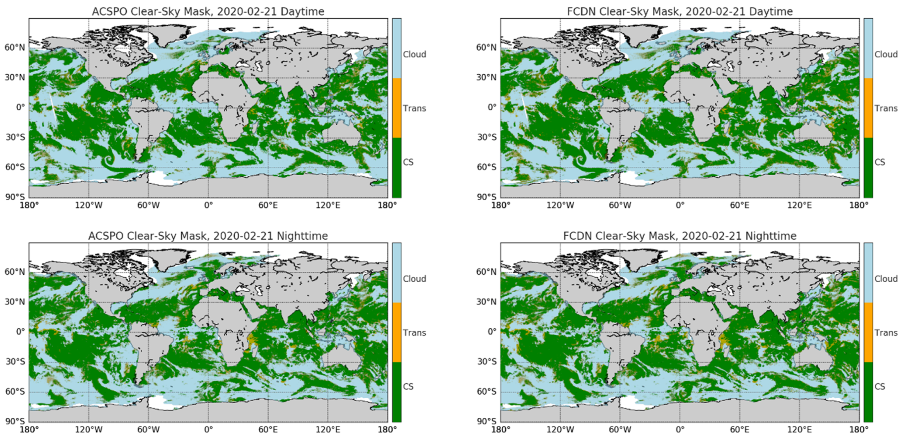
Figure 1 shows the global distribution of the ACSPO CSM and the FCDN_CSM prediction on 21 February 2020. The global distributions are quite consistent between the ACSPO CSM and the FCDN_CSM for both day and night, regardless of the latitude, coastal area, and sun glint area, which could involve rapid atmospheric and geophysical condition changes. Both CSMs are also consistent with the day true-color images and night images for VIIRS monitored on the ICVS web page. Note that the FCDN_CSM mainly focuses on clear-sky identification for improving the FCDN_CRTM performance. This is slightly different from cloud mask products, such as the VIIRS cloud mask (VCM) [10,11], which mainly analyzes cloud types and cloud radiometric characteristics. Therefore, the analyses of different cloud types are out of scope of this paper. With the exception of the F-score analyses in this section, we further validated the FCDN_CSM accuracy and stability by evaluating global O-M mean and standard deviations, and compared them with ACSPO CSM, as discussed in the next subsection.
3.2. Validation with O-M Biases
An evaluation of the VIIRS radiometric biases with the O-M biases for TEB bands has been conducted in earlier research [3,4,5,6]. Similarly, we used the analysis method of the O-M biases to evaluate ACSPO CSM [3], where the global O-M biases for TEB bands were calculated using the ACSPO CSM to identify clear-sky pixels, and the CSM was then evaluated by the O-M mean biases and STDs. As with the evaluation of ACSPO CSM, we also used O-M biases to evaluate FCDN_CSM accuracy and stability.
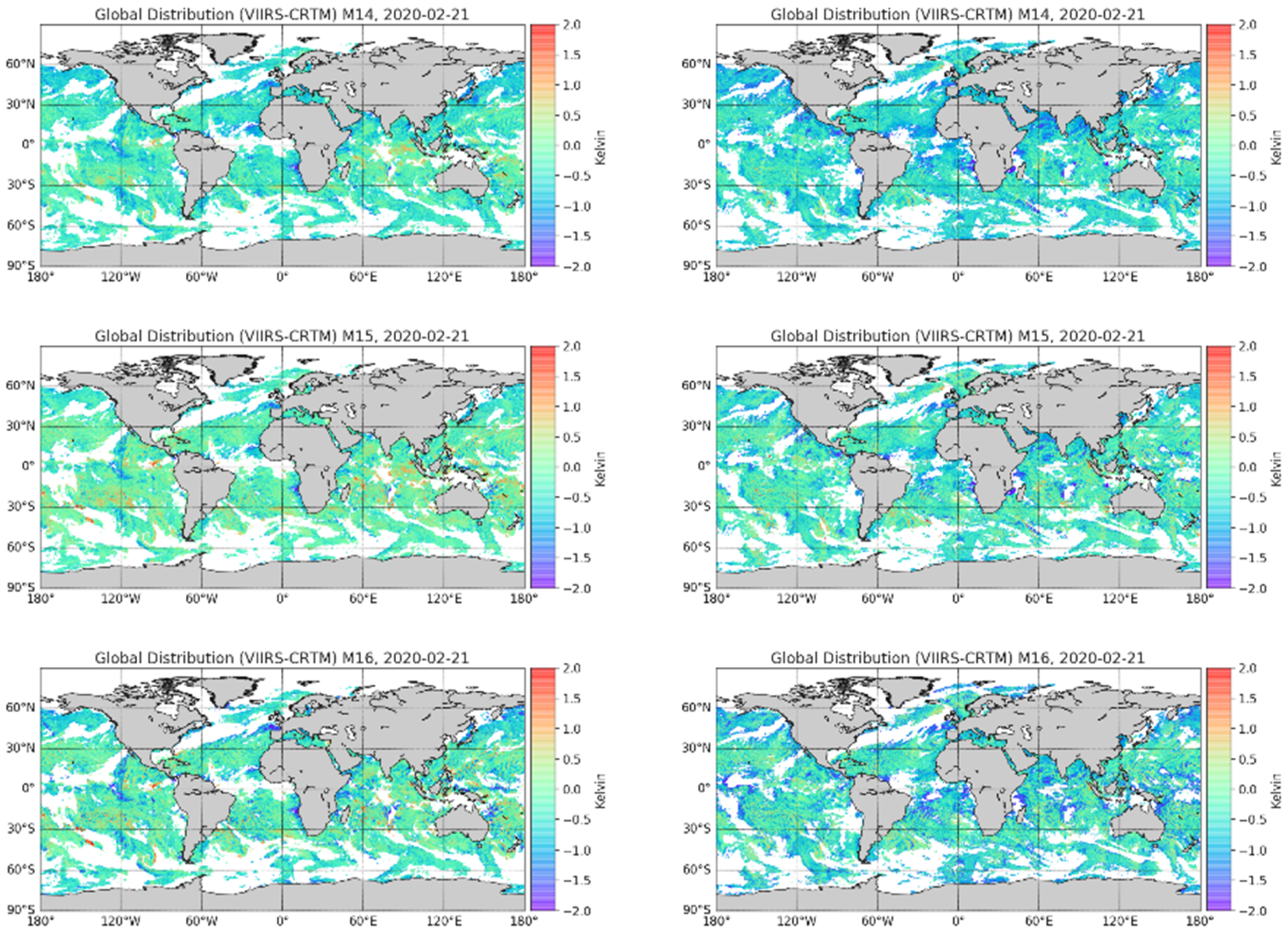
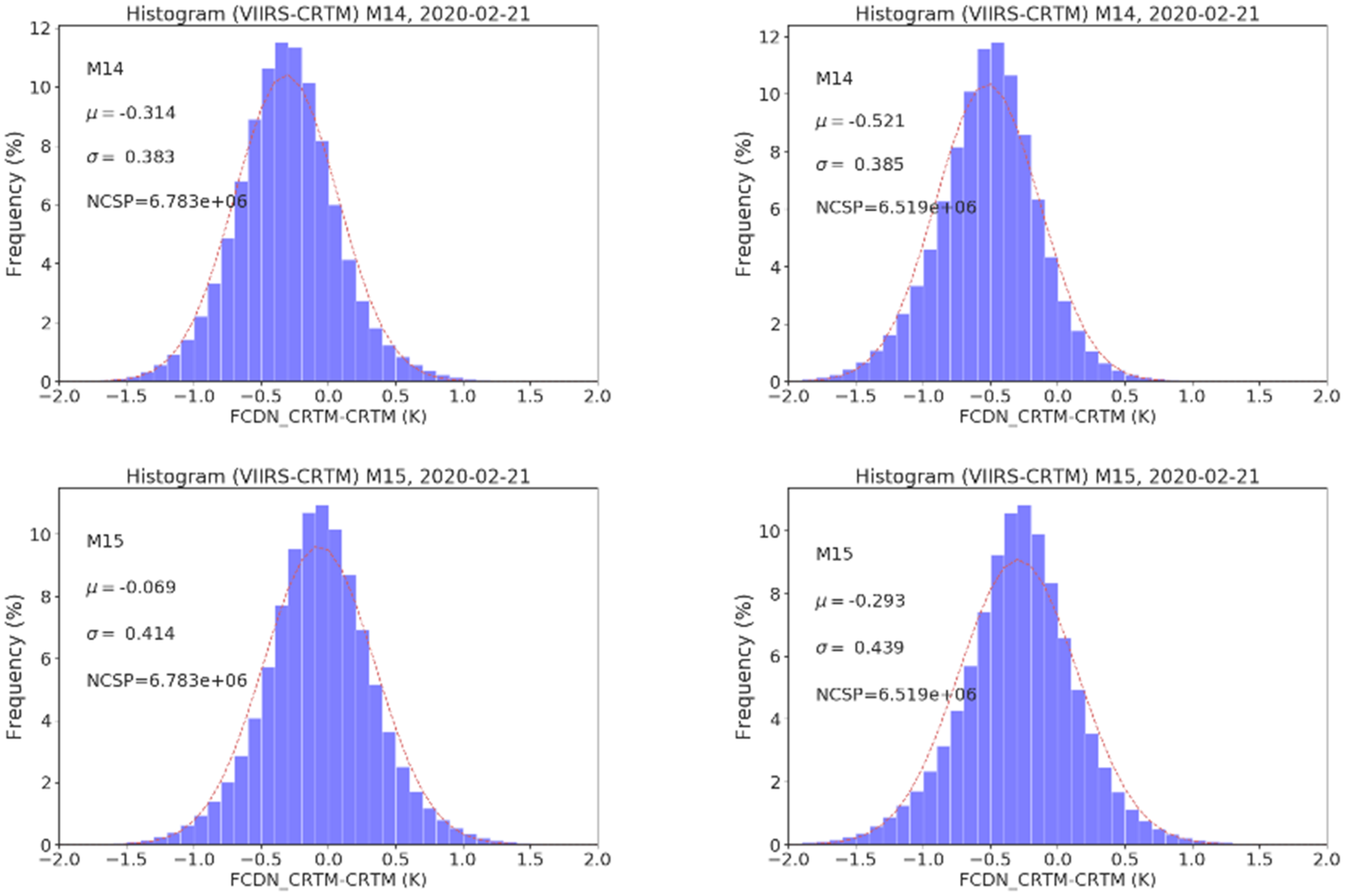
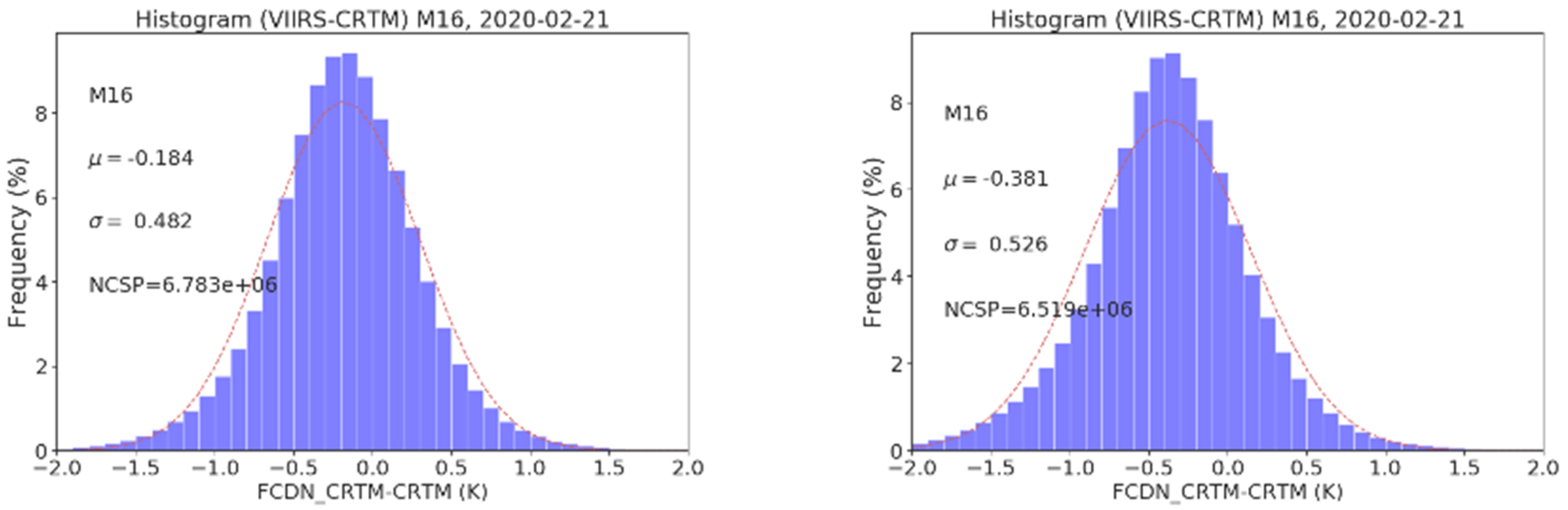
Table 5 shows the global O-M statistics corresponding to Figure 1, using the two CSMs to identify clear-sky pixels. Due to solar reflection contamination, M12 was not used in the daytime analysis. The global O-M mean biases of the FCDN_CSM and ACSPO are comparable for all bands and both day and night, suggesting that the predicted CSM is unbiased with respect to ACSPO CSM. STDs are also close to those of the ACSPO, although they are slightly worse for the three long wave IRs (LWIR): M14, M15, and M16. More detail about the accuracy of STD is provided below. Figure 2 and Figure 3 further show global distribution and histograms of the O-M biases for VIIRS M14, M15, and M16 for day and night using the FCDN_CSM as a clear-sky identification. The global distributions are uniform and the O-M mean biases in most areas are close to zero for both day and night. All histograms are Gaussian distributed. The O-Ms in daytime are slightly warmer than at night, as expected, due to the pronounced daytime diurnal cycle, which was not taken into account in the CRTM simulation [3].
All global statistics and distribution of O-M biases are generally consistent with those of ACSPO CSM, with the exception of the STDs, which are slightly worse for LWIRs; these decreased from 0.032 K in M14 to 0.045 K in M16 in nighttime, and from 0.033 K in M14 to 0.055 K in M16 in daytime. As shown in the table, one reason for the slight STD degradation in LWIRs is because the number of clear-sky pixels predicted by the FCDN_CSM model ranges from 2.3% (day) to 3.3% (night) larger than that in the ACSPO CSM, which may attribute to residual cloud in the FCDN_CSM model. However, this is not the only case. Type Cloud generally occupies ~80% of the total pixels—about four times larger than type CS and more than ten times larger than type Transition. Although the Cloud predictions were highly accurate, the 97% recall (Table 3 and Table 4) means that there remains a 3% misidentification, which was distributed to CS or Transition, resulting in a slight degradation in precision for type CS, and significant accuracy reduction for type Transition. As a result, ~9% and ~7% pixels were misjudged as CS for day and night, respectively, as shown in Table 3 and Table 4. This clearly does not mean that all misjudgments in CS are real Cloud or PCS types. An offline analysis of a subset of the 3% misidentification in Cloud showed that the O-M biases were very close to zero, and more similar to CS than to Cloud. This indicates that the ACSPO CSM algorithm may be somewhat conservative, as discussed in [1], resulting in misjudgment of some CS pixels as Cloud in ACSPO, which was corrected by the FCDN_CSM prediction.
Overall, some room still exists to improve FCDN_CSM in the future. Although one might think that increasing the amount of Transition and CS in the training data set would be a solution to improve the identification accuracies of the model, extensive experiments have been conducted and shown that this is not the case. As we discussed in the previous subsection, the root source of this cloud misidentification may be inadequate consideration of the surrounding effects for each pixel in the current FCDN_CSM model, because Cloud and PCS are partly tested by the radiative variation of the surrounding pixels [1,11]. Further fine-tuning of the model is needed to improve the CSM identification accuracy, particularly for the remaining 3% misidentification in the recall for type Cloud. Further discussion about this issue is provided in Section 4.
Nevertheless, both recall and precision for CS are highly accurate (>90%) for both daytime and nighttime, and the largest degradation in STDs (~0.055 K) is still within the range of the FCDN_CRTM validation. Furthermore, similar to the case of v1 [14], using a NOAA internal Linux server with 100 G memory and 2.2 G multi-core CPUs and without GPU support, the FCDN-CSM v2 takes about 20 s to generate one day of CSM (about 0.6 billion pixels), excluding the calculation of CWV and other atmosphere parameters, whereas the updated ACSPO v2.4 needs more than five hours to obtain the same CSM product. This high efficiency, together with the high accuracies in F-score and O-M biases, render the FCDN_CSM a better selection as the clear-sky identification for the FCDN_CRTM.
3.3. Stability of the FCDN_CSM
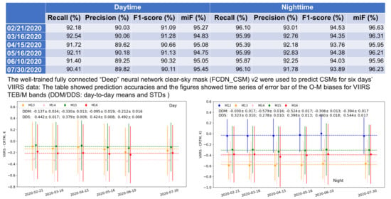
To check the stability of the FCDN_CSM, we used FCDN_CSM v2 to predict CSM and analyzed O-M biases for the other five dispersion days (16 March 2020, 15 April 2020, 16 May 2020, 10 June 2020, and 30 July 2020), which comprise nearly one day per month selected from March to July in 2020. Including 21 February 2020, a total of six days’ data were used to evaluate the stability of the FCDN_CSM. Note that all days’ selection was random. We did not apply any specific conditions to these days. Input, correct, and F1-score results for type CS, together with corresponding recall, precision, and overall miF, are listed in Table 6 and Table 7. The F1-score is Fβ-score when β is equal to one, giving the same weight to recall and precision. Note that while miF is used to check overall FCDM_CSM performance, the other parameters in the tables are only for type CS, as only CS is needed for the FCDN_CRTM validation.
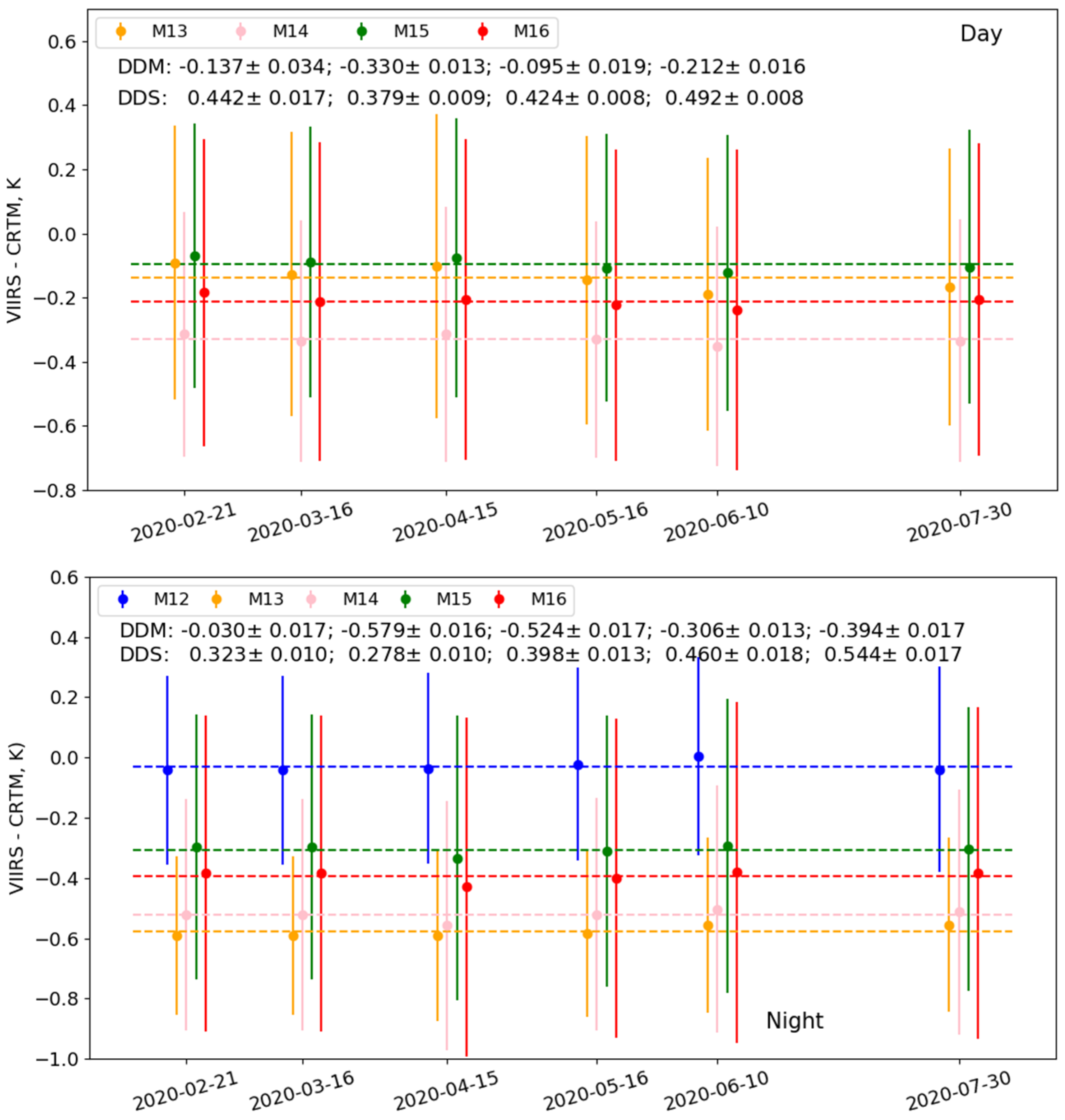
Recall, precision, and F1-score are generally consistent for all five days (both daytime and nighttime). The typical values are 92%, 90%, and 91% for daytime and 96%, 92%, and 94% for nighttime, respectively. All statistical values are comparable with the high accuracies of 21 February 2020, although there are minor degradations with the time in some parameters at the end of the analysis period. For instance, the maximum degradations are in daytime recall and nighttime precision, which decreased by ~2.1% and ~1.2% on 30 July 2020—about half a year from the selected training data set. As expected, both recall and precision for nighttime are 2–4% higher than those of daytime for every analysis period, making the F1-score and the miF ~3% and ~1% higher. Furthermore, miF persists at ~95% for day and ~96% for night, suggesting not only that the CS type has high prediction accuracy and stability, but also that Cloud has great accuracy, and both Cloud and Transition are quite stable in time. The global O-M distributions and corresponding histograms for the latter five days were similar to those of 21 February 2020—global distributions of the O-M mean biases are uniform and close to zero, and the corresponding histograms are Gaussian distributed, as shown in Figure 2 and Figure 3. Figure 4 shows the error bars of the VIIRS O-M biases for six dispersion days from February to July 2020 for daytime and nighttime, where the VIIRS clear-sky pixels were identified by FCDN_CSM v2. Two-line statistics values show the day-to-day means (DDM) and STDs (DDS) of the O-M mean biases and STDs for each corresponding band, as a check on the temporal and spatial variability of the O-M biases. The dashed lines represent the DDMs for each band. The O-M mean biases are consistent with the corresponding DDM lines, with uncertainty within several thousandths of a Kelvin for both daytime and nighttime, and STD uncertainty is similar. This result suggests the O-M biases are generally stable over time. This high stability also indicates that there is no significant overfitting in the FCDN_CSM v2.
4. Discussion
Due to the high prediction accuracies, efficiency, and stability, at the time of writing, the FCDN_CSM v2 has been successfully used for the FCDN_CRTM as clear-sky identification to predict VIIRS clear-sky radiances for five TEB/M bands. The result was documented in the companion paper—Part 2 and previously published [23]. In addition, we were also exploring possible means to improve the model, which is discussed in this section.
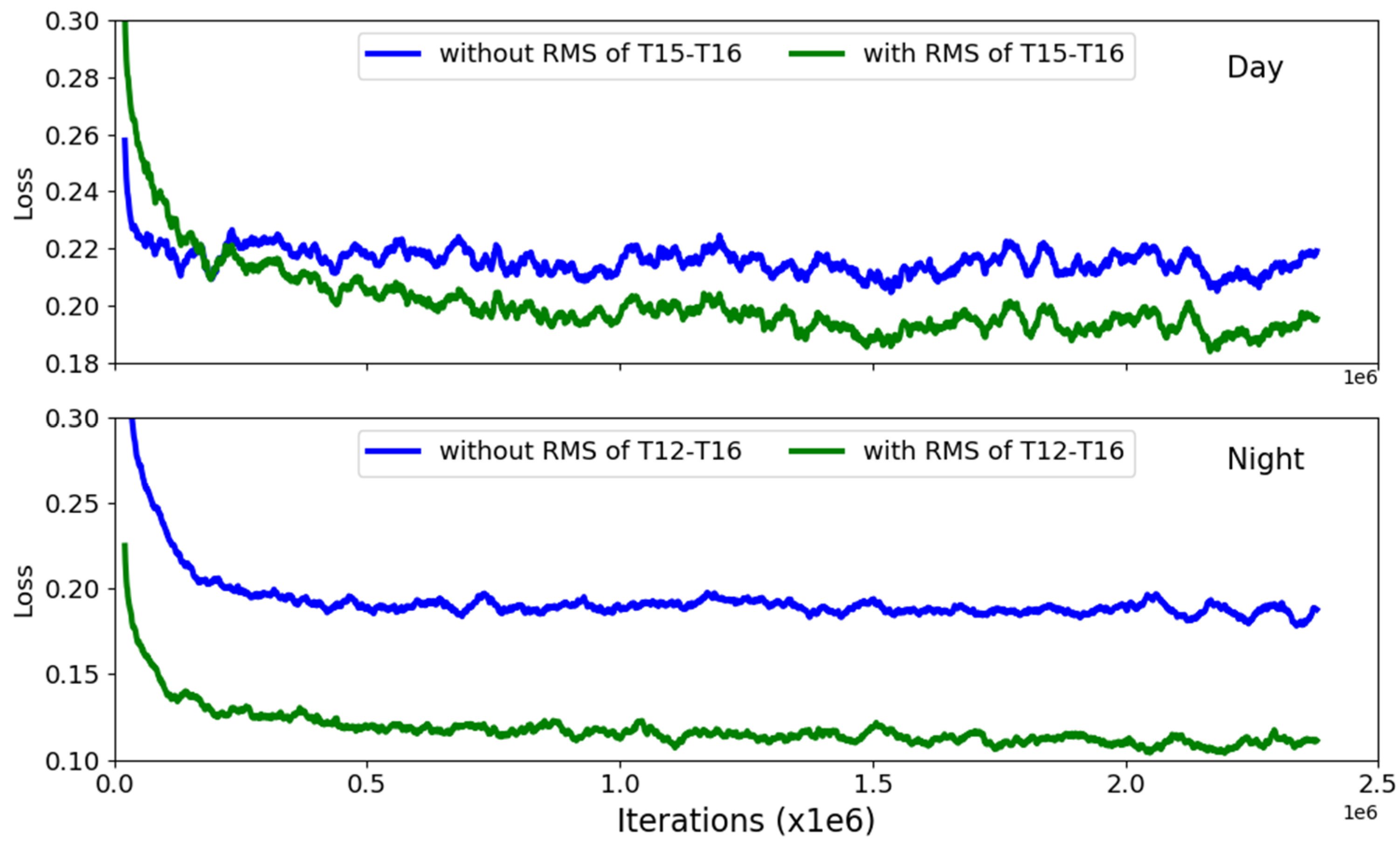
As discussed in the previous section, the slightly worse accuracy in type Transition, mainly resulting from a 3% misidentification from type Cloud, appears to be partly due to the inadequate consideration of spatial variance in FCDN_CSM, because Cloud and PCS are partly tested by the variation in the surrounding pixels [1,11]. This raises questions about how to verify this hypothesis, and whether any potential improvement can be made to the FCDN_CSM prediction accuracy. Because the FCDN_CSM architecture is relatively simple, and has only 13 and 10 input features for daytime and nighttime mode, and multiple experiments have been conducted to tune the number of layers and neurons and other hyperparameters during the model training and testing, it is unlikely that the model’s accuracy can be further improved by continued tuning of the model. Recall that in FCDN_CSM v1, we conducted a sensitivity analysis about the selection of important features and successfully improved the model’s efficiency without significant loss of accuracy [15]. Thus, the selection of features may still have the potential to provide a means to improve FCDN_CSM prediction accuracy and verify our hypothesis above. Therefore, in this section, we tested a new feature—a root mean square (RMS) of BT difference, which represents spatial radiative variability in FCDN_CSM, in addition to the individual BTs as the model inputs. The BT difference between M15 and M16 (T15–16) was used for daytime, and the BT difference between M12 and M16 (T12–16) for nighttime. As is well-known, T12–16 and T15–16 are comprehensively used in the cloud mask algorithm to assist in the classification of CS and semitransparent clouds, by exploiting radiative properties of clouds in the thermal IR spectral range [1,11,12]. Both T12–16 RMS (RMS12–16) and T15–16 RMS (RMS15–16) were calculated from a 40 × 40 moving window around each pixel. We retrained the model using the same six days’ data as described in Section 2, but added RMS12–16 for nighttime and RMS15–16 for daytime as a new feature. Figure 5 shows the changes to the cost functions during the model training with comparison to the cases without the new feature, which have the same number of input features as the FCDN_CSM v2 listed in Table 1. It is clear that, in the daytime, the cost functions for the case with the RMS15–16 are larger in the first 200,000 iterations. However, after the model was trained adequately, the cost functions became smaller than those without the RMS, and the cost further declined at the end of the training. For nighttime, the cost function for the case with the RMS12–16 is persistently smaller than that without the RMS and the amplitude is significantly larger than that of the daytime. Both cost reductions suggest that the model biases could be further reduced by adding the RMS12–16 and RMS15–16, and the reduction in nighttime is more pronounced than that in daytime.
Table 8 shows recall (R) and precision (P) for three CSM types in test data between the cases of with and without RMS12–16 and RMS15–16, for both daytime and nighttime. The miF and maF are also provided. The precisions of the type Cloud are more than 99.6% for all cases and are consistent between the cases with and without the new feature. However, for the cases with the new feature, the recall of type Cloud increases 0.45% (97.91—97.46%) in daytime and 1.18% (98.18–97.00%) in nighttime. Thus, the misidentification in Cloud is reduced from 3% to 2.5% and 1.82% for daytime and nighttime, respectively, which reduces the Cloud contamination to the other two types, and thus improves the recall and precision for both CS and Transition, particularly for nighttime. The precision of Transition and CS increases from 72.04% and 92.94% to 78.17% and 95.51%, respectively. As a result, miF for the cases with the new feature increases by 0.43% for daytime and 1% for nighttime, and maF increases by 1% for day and 2% for night. The O-M mean biases and STDs in each case are listed in Table 9. As expected, the means are comparable between the cases with and without the new feature, but the STDs are improved for all bands, especially for the nighttime M16, where the STDs were reduced by 0.04 K. Overall, selection of features is a potential means to improve the model accuracy. Because the FCDN_CSM v2 has been used for FCDN_CRTM to predict clear-sky radiances for VIIRS TEB/M bands and the related results have been published [23], and currently the evaluation of this new feature did not reach full maturity, we decided to add the RMS feature to the next version of FCDN_CSM (v3), rather than to v2, and the accuracies and stabilities for both ocean and land will be re-evaluated.
In addition to prediction accuracy, long-term stability is also a critical factor of the FCDN_CSM performance that needs to be carefully evaluated. At the time of writing, the selected prediction data were only accumulated until 30 July 2020, which covered half a year from the end of the selected training data period. During the whole evaluation period, the FCDN_CSM v2 showed long-term stability for both O-M mean biases and STDs, and obviously outperforms v1, for which a period of stability of only several weeks appeared. Although further validation of the model stability is needed by accumulating recent or future data, the degradations in daytime recall and nighttime precision in 30 July 2020 (Table 6 and Table 7) imply that the stability of the FCDN_CSM v2 may degrade for a more extended prediction period. Therefore, it is still necessary to consider potential means to improve future model stability. The discussion below aims to achieve this purpose. First, time and location, which were not included in the FCDN_CSM v2, may be two potential features to improve long term stability. Second, we noted that the addition of the new RMS feature can improve prediction accuracies. It is also possible to improve the stability by further checking the stability using the other five days’ data. Third, using more data for training may be another means to improve model stability. In addition, the model architecture can still be fine-tuned to further avoid model overfitting. Finally, similar to the case of FCDN_CRTM, retraining the model periodically is also a substitute method to maintain long-term stability of the model.
One advantage of the FCDN_CSM is migration capability, that is, the NOAA-20 VIIRS CSM will be predicted directly using the well-trained FCDN_CSM v2 by S-NPP data. This advantage has been demonstrated in detail in the FCDN_CSM v1 [14]. Because the design, data preprocessing, training, and testing for v2 are quite similar to those for v1, the migration advantage could be applied to v2. Indeed, further quantitative validation is needed to check the prediction accuracies and stability for NOAA-20, and we will re-evaluate the migration advantage quantitatively in the next version.
5. Conclusions
An earlier-developed FCDN_CSM was reviewed and enhanced to improve its stability, in addition to its accuracy and efficiency. This enhanced model is referred to as FCDN_CSM v2. In addition, daytime analysis was included in v2. The objective was to develop a fast and robust FCDN_CSM for CS identification for the FCDN_CRTM model. Six dispersion days of data, covering all seasons, were selected as the model inputs to improve model stability. Because the input data covers all seasons and more features are used for daytime, the model architecture was redesigned to include three hidden layers with 32 × 64 × 16 neurons for both nighttime and daytime to be trained adequately. The input features were extracted from the VIIRS SDR data, in conjunction with ECMWF and CMC SST. The well-trained model was then used to predict six dispersion days’ data in 2020 as an accuracy and stability check.
Based on the analyses of the F-score, which is commonly used to evaluate the performance of classification problems, of the three CSM types predicted in the FCDN_CSM v2, type Cloud was the most accurate, showing ~97% recall and more than 99% precision for both daytime and nighttime. This was followed by the type Clear-Sky, which showed ~96% recall and ~93% precision in the nighttime, and was ~3% worse in the daytime. The high prediction accuracies persisted in all prediction days, with the exception of slight degradations (~2.1% daytime recall and ~1.2% nighttime precision) for the last prediction day, which lay about half a year from the time of the training data. The O-M mean biases are comparable with the ACSPO CSM for all bands, as are the STDs of the short-wave IRs (M12 and M13); whereas the standard deviations (STD) were slightly degraded in long wave IRs (M14, M15 and M16), indicating that residual cloud or outliers may have existed in the FCDN_CSM. Thus, further fine-tuning to improve the O-M biases may be required in the future. An improvement for the model was discussed, which uses an RMS of the BT difference as a new input feature to represent the spatial radiative variability around each pixel. Overall, the consistent O-M means and STDs for whole prediction periods proved that the FCDN_CSM v2 is robust and does not have significant overfitting. Combined with the excellent F-scores, stability, high efficiency, and allowable STDs, the FCDN_CSM version 2 has been successfully used for the FCDN_CRTM to predict VIIRS clear-sky radiances for five TEB/M bands [23]. Our future work will extend the FCDN_CSM functionalities to include land analysis.
Author Contributions
X.L. developed methods, created the evaluation dataset, analyzed results and wrote the manuscript. Q.L. supervised research and technique guide. All authors have read and agreed to the published version of the manuscript.
Funding
This research was funded by NOAA grant NA14NES4320003 (Cooperative Institute for Satellite Earth System Studies-CISESS) at the Earth System Science Interdisciplinary Center of University of Maryland.
Institutional Review Board Statement
Not applicable.
Informed Consent Statement
Not applicable.
Data Availability Statement
Not applicable.
Acknowledgments
CRTM and ACSPO are provided by the CRTM and SST teams of NOAA STAR. The authors thank Alexander Ignatov, Changyong Cao, and Sid Boukabara for advice and help. We also thank Christopher Grassotti and the STAR MiRS Team for technical discussions and suggestions. The views, opinions, and findings contained in this report are those of the authors and should not be construed as an official NOAA or U.S. Government position, policy, or decision.
Conflicts of Interest
The authors declare no conflict of interest.
References
- Petrenko, B.; Ignatov, A.; Kihai, Y.; Heidinger, A. Clearsky mask for the Advanced Clear-Sky Processor for Oceans. J. Atmos. Ocean. Technol. 2010, 27, 1609–1623. [Google Scholar] [CrossRef]
- Yu, Y.; Privette, J.L.; Pinheiro, A.C. Analysis of the NPOESS VIIRS land surface temperature algorithm using MODIS data. IEEE Trans. Geosci. Remote Sens. 2005, 43, 2340–2350. [Google Scholar] [CrossRef]
- Liang, X.; Ignatov, A.; Kihai, Y. Implementation of the Community Radiative Transfer Model (CRTM) in Advanced Clear-Sky Processor for Oceans (ACSPO) and validation against nighttime AVHRR radiances. J. Geophys. Res. 2009, 114, D06112. [Google Scholar] [CrossRef]
- Liang, X.; Ignatov, A. Monitoring of IR Clear-sky Radiances over Oceans for SST (MICROS). J. Atmos. Ocean. Technol. 2011, 28. [Google Scholar] [CrossRef] [Green Version]
- Liang, X.; Ignatov, A. AVHRR, MODIS, and VIIRS radiometric stability and consistency in SST bands. J. Geophys. Res. 2013, 118. [Google Scholar] [CrossRef]
- Liang, X.; Ignatov, A. Preliminary Inter-Comparison between AHI, VIIRS and MODIS Clear-Sky Ocean Radiances for Accurate SST Retrievals. Remote Sens. 2016, 8, 203. [Google Scholar] [CrossRef] [Green Version]
- Wang, H.; Fuller-Rowell, T.J.; Akmaev, R.A.; Hu, M.; Kleist, D.T.; Iredell, M.D. First simulations with a whole atmosphere data assimilation and forecast system: The January 2009 major sudden stratospheric warming. J. Geophys. Res. 2011, 116, A12321. [Google Scholar] [CrossRef]
- Liu, Q.; Delst, P.V.; Chen, Y.; Groff, D.; Han, Y.; Collard, A.; Weng, F. Community radiative transfer model for radiance assimilation and applications. In Proceedings of the 2012 IEEE International Geoscience and Remote Sensing Symposium, Munich, Germany, 22–27 July 2012; pp. 3700–3703. [Google Scholar]
- Liu, Q.; Boukabara, S. Community Radiation Transfer Model (CRTM) Applications in Supporting the Suomi National Polar-Orbiting Partnership (SNPP) Mission validation and Verification. Remote Sens. Environ. 2014, 140, 744–754. [Google Scholar] [CrossRef]
- Kopp, T.J.; Thomas, W.; Heidinger, A.K.; Botambekov, D.; Frey, R.A.; Hutchison, K.D.; Iisager, B.D.; Brueske, K.; Reed, B. The VIIRS Cloud Mask: Progress in the first year of S-NPP toward a common cloud detection scheme. J. Geophys. Res. Atmos. 2014, 119, 2441–2456. [Google Scholar] [CrossRef]
- Heidinger, A.K.; Evan, A.T.; Foster, M.J.; Walther, A. A Naive Bayesian Cloud-Detection Scheme Derived from CALIPSO and Applied within PATMOS-x. J. Appl. Meteor. Climatol. 2012, 51, 1129–1144. [Google Scholar] [CrossRef]
- Frey, R.A.; Ackerman, S.A.; Liu, Y.; Strabala, K.I.; Zhang, H.; Key, J.R.; Wang, x. Cloud Detection with MODIS. Part I: Improvements in the MODIS Cloud Mask for Collection 5. J. Atmos. Ocean. Technol. 2008, 25, 1057–1072. [Google Scholar] [CrossRef]
- Stowe, L.L.; Davis, P.A.; McClain, E.P. Scientific basis and initial evaluation of the CLAVR-1 global clear/cloud classification algorithm for the Advanced Very High Resolution Radiometer. J. Atmos. Ocean. Technol. 1999, 16, 656–681. [Google Scholar] [CrossRef]
- Liang, X.; Liu, Q.; Yan, B.; Sun, N. A Deep Learning Trained Clear-Sky Mask Algorithm for VIIRS Radiometric Bias Assessment. Remote Sens. 2020, 12, 78. [Google Scholar] [CrossRef] [Green Version]
- Wang, C.; Platnick, S.; Meyer, K.; Zhang, Z.; Zhou, Y. A machine-learning-based cloud detection and thermodynamic-phase classification algorithm using passive spectral observations. Atmos. Meas. Tech. 2020, 13, 2257–2277. [Google Scholar] [CrossRef]
- Ball, J.E.; Anderson, D.T.; Chan, C.S. Comprehensive survey of deep learning in remote sensing: Theories, tools, and challenges for the community. J. Appl. Remote Sens. 2017, 11, 042609. [Google Scholar] [CrossRef] [Green Version]
- Krasnopolsky, V.M.; Fox-Rabinovitz, M.S.; Hou, Y.T.; Lord, S.J.; Belochitski, A.A. Accurate and Fast Neural Network Emulations of Model Radiation for the NCEP Coupled Climate Forecast System: Climate Simulations and Seasonal Predictions. Mon. Weather Rev. 2009, 138, 1822–1842. [Google Scholar] [CrossRef]
- Zhu, X.; Tuia, D.; Mou, L.; Xia, G.; Zhang, L.; Xu, F.; Fraundorfer, F. Deep Learning in Remote Sensing: A Comprehensive Review and List of Resources. IEEE Geosci. Remote Sens. Mag. 2017, 5, 8–36. [Google Scholar] [CrossRef] [Green Version]
- Boukabara, S.A.; Maddy, E.; Shahroudi, N.; Hoffman, R.N.; Connor, T. Artificial Intelligence (AI) Techniques to Enhance Satellite Data Use for Nowcasting and NWP/Data Assimilation. In Proceedings of the 100th American Meteorological Society Annual Conference, Boston, MA, USA, 12–16 January 2020. [Google Scholar]
- NOAA. NOAA Artificial Intelligence (AI) Strategy. February 2020. Available online: https://nrc.noaa.gov/LinkClick.aspx?fileticket=0I2p2-Gu3rA%3D&tabid=91&portalid=0 (accessed on 8 January 2021).
- Li, Z.; Shen, H.; Cheng, Q.; Liu, Y.; You, S.; He, Z. Deep learning based cloud detection for medium and high resolution remote sensing images of different sensors. Isprs J. Photogramm. Remote Sens. 2019, 150, 197–212. [Google Scholar] [CrossRef] [Green Version]
- Liang, X.; Sun, N.; Ignatov, A.; Liu, Q.; Wang, W.; Zhang, B.; Weng, F.; Cao, C. Monitoring of VIIRS ocean clear-sky brightness temperatures against CRTM simulation in ICVS for TEB/M bands. Proc. SPIE Earth Obs. Syst. XXII 2017, 104021S. [Google Scholar] [CrossRef]
- Liang, X.; Liu, Q. Applying Deep Learning to Clear-Sky Radiance Simulation for VIIRS with Community Radiative Transfer Model—Part 2: Model Training, Test and validation. Remote Sens. 2020, 12, 3825. [Google Scholar] [CrossRef]
- Liang, X.; Ignatov, A. Validation and Improvements of Daytime CRTM Performance Using AVHRR IR 3.7 µm Band. In Proceedings of the 13th AMS on Conference Atmospheric Radiation, Portland, OR, USA, 28 June–2 July 2010; Available online: https://ams.confex.com/ams/pdfpapers/170593.pdf (accessed on 8 January 2021).
- Liang, S. Narrowband to broadband conversions of land surface albedo I: Algorithms. Remote Sens. Environ. 2001, 76, 213–238. [Google Scholar] [CrossRef]
- Borbas, E.E.; Hulley, G.; Feltz, M.; Knuteson, R.; Hook, S. The Combined ASTER MODIS Emissivity over Land (CAMEL) Part 1: Methodology and High Spectral Resolution Application. Remote Sens. 2018, 10, 643. [Google Scholar] [CrossRef] [Green Version]
- Heidinger, A.; Botambekov, D.; Walther, A. A Naïve Bayesian Cloud Mask Delivered to NOAA Enterprise. Ver. 1.2. 2016. Available online: https://www.star.nesdis.noaa.gov/goesr/documents/ATBDs/Enterprise/ATBD_Enterprise_Cloud_Mask_v1.2_Oct2016.pdf (accessed on 8 January 2021).
- Ng, A.Y. Feature selection, L1 vs. L2 regularization, and rotational invariance. In Proceedings of the 21st International Conference on Machine Learning (ICML ’04), Banff, AB, Canada, 4–8 July 2004. [Google Scholar]
- Lipton, Z.C.; Elkan, C.; Narayanaswamy, B. Optimal Thresholding of Classifiers to Maximize F1 Measure. In Proceedings of the Machine Learning and Knowledge Discovery in Databases: European Conference, Skopje, North Macedonia, 18–22 September 2014; Volume 8725, pp. 225–239. [Google Scholar]
- Yang, Y. An Evaluation of Statistical Approaches to Text Categorization. Inf. Retr. 1999, 1, 69–90. [Google Scholar] [CrossRef]
- Zhang, D.; Wang, J.; Zhao, X. Estimating the uncertainty of average F1 scores. In Proceedings of the 2015 International Conference on The Theory of Information Retrieval (ICTIR ’15), Northampton, MA, USA, 27–30 September 2015; pp. 317–320. Available online: https://core.ac.uk/download/pdf/141223586.pdf (accessed on 8 January 2021).
Figure 1.
Global distribution of CSM types Advanced Clear-Sky Processor over Ocean (ACSPO) (actual) and FCDN_CSM (predicted) on 21 February 2020, including Clear-Sky pixels (CS), cloud pixels (Cloud), and transition pixels between Clear-Sky and Cloud (Trans).
Figure 1.
Global distribution of CSM types Advanced Clear-Sky Processor over Ocean (ACSPO) (actual) and FCDN_CSM (predicted) on 21 February 2020, including Clear-Sky pixels (CS), cloud pixels (Cloud), and transition pixels between Clear-Sky and Cloud (Trans).

Figure 2.
Global distribution of the O-M biases on 21 February 2020 for VIIRS M14 (top), M15 (middle), and M16 (bottom), using FCDN_CSM as clear-sky identification for both daytime (left) and nighttime (right).
Figure 2.
Global distribution of the O-M biases on 21 February 2020 for VIIRS M14 (top), M15 (middle), and M16 (bottom), using FCDN_CSM as clear-sky identification for both daytime (left) and nighttime (right).

Figure 3.
Histograms of the O-M biases on 21 February 2020 for VIIRS M14 (top), M15 (middle), and M16 (bottom), using FCDN_CSM as clear-sky identification for both daytime (left) and nighttime (right).
Figure 3.
Histograms of the O-M biases on 21 February 2020 for VIIRS M14 (top), M15 (middle), and M16 (bottom), using FCDN_CSM as clear-sky identification for both daytime (left) and nighttime (right).


Figure 4.
The error bars of the Visible Infrared Imaging Radiometer Suite (VIIRS) O-M biases for six dispersion days from February to July 2020 for day (upper) and night (bottom). The VIIRS clear-sky pixels were identified by FCDN_CSM. Two-line statistics values present the day-to-day means (DDM) and STDs (DDS) of the O-M means and STDs for each corresponding band ordered from M13 to M16 for daytime and from M12 to M16 for nighttime. The dashed lines represent the DDMs for each band.

Figure 5.
The changes in cost function for day (upper) and night (bottom) during FCDN_CSM training with and without the RMS12–16 or RMS15–16 as a new feature.
Figure 5.
The changes in cost function for day (upper) and night (bottom) during FCDN_CSM training with and without the RMS12–16 or RMS15–16 as a new feature.


Table 1.
Summary of input features and output clear-sky mask (CSM) types in the fully connected deep neural network CSM (FCDN_CSM) v2.
Table 1.
Summary of input features and output clear-sky mask (CSM) types in the fully connected deep neural network CSM (FCDN_CSM) v2.
| Day | Night | |
|---|---|---|
| Common Input Features | Satellite Zenith Angle (SZA), Column Water Vapor Contents (CWV), Surface Air Temperature (SAT), Surface Water Vapor contents (SWV), M15 BT, M16 BT, Regression SST (REG_SST), Reference SST (REF_SST), SST Spatial Variance (SSV) | |
| Input Features Only for Day or Night | M12 BT | M5 albedo |
| M7 albedo | ||
| Glint-angle spatial variance (GSV) | ||
| Solar Zenith Angle (SOZA) | ||
| Output CSM Types | Clear-Sky, Transition, Cloud | |
Table 2.
Summary of the VIIRS bands used in the FCDN_CSM v2.
| Band Number | Wavelength (µm) | Spectral Range (µm) | Primary Uses |
|---|---|---|---|
| M5 | 0.672 | 0.662–0.682 | Day |
| M7 | 0.865 | 0.846–0.885 | Day |
| M12 | 3.70 | 3.660–3.840 | Night |
| M15 | 10.763 | 10.263–11.263 | Day and Night |
| M16 | 12.013 | 11.538–12.488 | Day and Night |
Table 3.
Summary of evaluation of three CSM types in nighttime, 21 February 2020.
| Input | Correct | Prediction | Recall (%) | Precision (%) | |
|---|---|---|---|---|---|
| CS | 6,309,189 | 6,063,150 | 6,518,594 | 96.10 | 93.01 |
| Transition | 2,121,462 | 1,925,740 | 2,664,887 | 90.77 | 72.26 |
| Cloud | 29,553,499 | 28,714,035 | 28,800,669 | 97.16 | 99.70 |
| Total/Average | 37,984,150 | 36,702,925 | 37,984,150 | 94.68 | 88.32 |
| miF and maF (%) | 96.63 | 91.14 | |||
Table 4.
Summary of evaluation of three CSM types in daytime, 21 February 2020.
| Input | Correct | Prediction | Recall (%) | Precision (%) | |
|---|---|---|---|---|---|
| CS | 6,623,885 | 6,106,453 | 6,782,545 | 92.19 | 90.03 |
| Transition | 2,283,160 | 1,832,188 | 2,802,059 | 80.25 | 65.39 |
| Cloud | 27,933,110 | 27,157,602 | 27,255,551 | 97.22 | 99.64 |
| Total/Average | 36,840,155 | 35,096,243 | 36,840,155 | 90.00 | 85.02 |
| miF and maF (%) | 95.27 | 87.19 | |||
Table 5.
Global O-M statistics for 21 February 2020 day and night in the bands M12–M16 with clear-sky identification using ACSPO CSM and FCDN_CSM. (µ: O-M mean; σ: O-M standard deviation; NCSP: the number of clear-sky pixels).
Table 5.
Global O-M statistics for 21 February 2020 day and night in the bands M12–M16 with clear-sky identification using ACSPO CSM and FCDN_CSM. (µ: O-M mean; σ: O-M standard deviation; NCSP: the number of clear-sky pixels).
| Nighttime | Daytime | |||||||
|---|---|---|---|---|---|---|---|---|
| ACSPO | FCDN_CSM | ACSPO | FCDN_CSM | |||||
| µ | σ | µ | σ | µ | σ | µ | σ | |
| M12 | −0.0281 | 0.2900 | −0.0405 | 0.3146 | N/A | N/A | N/A | N/A |
| M13 | −0.5805 | 0.2500 | −0.5894 | 0.2640 | −0.0808 | 0.4267 | −0.0912 | 0.4265 |
| M14 | −0.5246 | 0.3513 | −0.5213 | 0.3835 | −0.3156 | 0.3477 | −0.3141 | 0.3808 |
| M15 | −0.3026 | 0.4006 | −0.2933 | 0.4370 | −0.0736 | 0.3688 | −0.0690 | 0.4122 |
| M16 | −0.3958 | 0.4760 | −0.3812 | 0.5233 | −0.1927 | 0.4232 | −0.1841 | 0.4797 |
| NCSP | 6,309,189 | 6,518,594 | 6,623,885 | 6,782,545 | ||||
Table 6.
Summary of the FCDN_CSM daytime predictions for six days’ data.
| Input | Correct | Recall (%) | Precision (%) | F1-Score (%) | miF (%) | |
|---|---|---|---|---|---|---|
| 21 February 2020 | 6,623,885 | 6,106,453 | 92.18 | 90.03 | 91.09 | 95.27 |
| 16 March 2020 | 6,648,601 | 6,152,427 | 92.54 | 90.06 | 91.28 | 94.83 |
| 15 April 2020 | 6,325,957 | 5,802,787 | 91.72 | 89.62 | 90.66 | 95.08 |
| 16 May 2020 | 6,321,889 | 5,823,135 | 92.11 | 90.18 | 91.13 | 94.75 |
| 10 June 2020 | 5,860,868 | 5,356,848 | 91.40 | 89.25 | 90.32 | 95.05 |
| 30 July 2020 | 6,066,212 | 5,484,928 | 90.41 | 89.82 | 90.11 | 95.45 |
Table 7.
Summary of the FCDN_CSM nighttime predictions for six days’ data.
| Input | Correct | Recall (%) | Precision (%) | F1-Score (%) | miF (%) | |
|---|---|---|---|---|---|---|
| 21 February 2020 | 6,309,189 | 6,063,150 | 96.10 | 93.01 | 94.53 | 96.63 |
| 16 March 2020 | 6,438,926 | 6,180,724 | 95.99 | 92.76 | 94.35 | 96.31 |
| 15 April 2020 | 6,306,972 | 6,016,344 | 95.39 | 92.18 | 93.76 | 95.95 |
| 16 May 2020 | 6,355,016 | 6,100,474 | 95.99 | 92.83 | 94.38 | 96.21 |
| 10 June 2020 | 6,031,163 | 5,782,167 | 95.87 | 92.25 | 94.03 | 95.96 |
| 30 July 2020 | 5,756,199 | 5,531,779 | 96.10 | 91.78 | 93.89 | 96.23 |
Table 8.
Prediction accuracies for test data using FCDN_CSM v2 or FCDN_CSM v2 plus new RMS feature as Clear-Scheme 2. RMS: FCDN_CSM v2 plus new RMS feature).
Table 8.
Prediction accuracies for test data using FCDN_CSM v2 or FCDN_CSM v2 plus new RMS feature as Clear-Scheme 2. RMS: FCDN_CSM v2 plus new RMS feature).
| Daytime | Nighttime | ||||||||
|---|---|---|---|---|---|---|---|---|---|
| FCDN_CSM v2 | v2 + RMS15–16 | FCDN_CSM v2 | v2 + RMS12–16 | ||||||
| R (%) | P (%) | R (%) | P (%) | R (%) | P (%) | R (%) | P (%) | ||
| CS | 92.06 | 90.58 | 91.46 | 91.90 | 95.97 | 92.94 | 95.99 | 95.51 | |
| Transition | 80.75 | 67.36 | 83.66 | 68.69 | 89.93 | 72.04 | 91.34 | 78.17 | |
| Cloud | 97.46 | 99.60 | 97.91 | 99.72 | 97.00 | 99.64 | 98.18 | 99.60 | |
| Total/Average | 90.09 | 85.85 | 90.82 | 86.76 | 94.30 | 88.20 | 95.17 | 91.09 | |
| miF (%) | 95.37 | 95.80 | 96.40 | 97.40 | |||||
| maF(%) | 87.91 | 88.74 | 91.15 | 93.09 | |||||
Table 9.
The O-M mean biases and STDs for test data for VIIRS bands M12–M16 using FCDN_CSM v2 or FCDN_CSM v2 plus new RMS feature as clear-sky identification (µ: O-M mean; σ: O-M standard deviation; v2+RMS: FCDN_CSM v2 plus new RMS feature).
Table 9.
The O-M mean biases and STDs for test data for VIIRS bands M12–M16 using FCDN_CSM v2 or FCDN_CSM v2 plus new RMS feature as clear-sky identification (µ: O-M mean; σ: O-M standard deviation; v2+RMS: FCDN_CSM v2 plus new RMS feature).
| Daytime | Nighttime | |||||||
|---|---|---|---|---|---|---|---|---|
| FCDN_CSM v2 | v2 + RMS15–16 | FCDN_CSM v2 | v2 + RMS12–16 | |||||
| µ | σ | µ | σ | µ | σ | µ | Σ | |
| M12 | N/A | N/A | N/A | N/A | −0.0270 | 0.3042 | −0.0263 | 0.2942 |
| M13 | −0.1091 | 0.4649 | −0.1059 | 0.4594 | −0.5779 | 0.2671 | −0.5834 | 0.2660 |
| M14 | −0.3597 | 0.3901 | −0.3549 | 0.3800 | −0.5549 | 0.4008 | −0.5617 | 0.3870 |
| M15 | −0.1083 | 0.4226 | −0.1035 | 0.4116 | −0.3242 | 0.4574 | −0.3260 | 0.4318 |
| M16 | −0.2285 | 0.4867 | −0.2228 | 0.4753 | −0.4210 | 0.5512 | −0.4179 | 0.5149 |
Publisher’s Note: MDPI stays neutral with regard to jurisdictional claims in published maps and institutional affiliations. |
© 2021 by the authors. Licensee MDPI, Basel, Switzerland. This article is an open access article distributed under the terms and conditions of the Creative Commons Attribution (CC BY) license (http://creativecommons.org/licenses/by/4.0/).
Share and Cite
MDPI and ACS Style
Liang, X.; Liu, Q. Applying Deep Learning to Clear-Sky Radiance Simulation for VIIRS with Community Radiative Transfer Model—Part 1: Develop AI-Based Clear-Sky Mask. Remote Sens. 2021, 13, 222. https://doi.org/10.3390/rs13020222
AMA Style
Liang X, Liu Q. Applying Deep Learning to Clear-Sky Radiance Simulation for VIIRS with Community Radiative Transfer Model—Part 1: Develop AI-Based Clear-Sky Mask. Remote Sensing. 2021; 13(2):222. https://doi.org/10.3390/rs13020222
Chicago/Turabian StyleLiang, Xingming, and Quanhua Liu. 2021. "Applying Deep Learning to Clear-Sky Radiance Simulation for VIIRS with Community Radiative Transfer Model—Part 1: Develop AI-Based Clear-Sky Mask" Remote Sensing 13, no. 2: 222. https://doi.org/10.3390/rs13020222
Note that from the first issue of 2016, this journal uses article numbers instead of page numbers. See further details here.