Automated Machine Learning for High-Throughput Image-Based Plant Phenotyping


1
Agriculture Victoria, Grains Innovation Park, 110 Natimuk Rd, Horsham, VIC 3400, Australia
2
Agriculture Victoria, AgriBio, Centre for AgriBioscience, 5 Ring Road, Bundoora, VIC 3083, Australia
3
School of Applied Systems Biology, La Trobe University, Bundoora, VIC 3083, Australia
4
Centre for Agricultural Innovation, School of Agriculture and Food, Faculty of Veterinary and Agricultural Sciences, The University of Melbourne, Melbourne, VIC 3010, Australia
*
Author to whom correspondence should be addressed.
Remote Sens. 2021, 13(5), 858; https://doi.org/10.3390/rs13050858
Submission received: 29 January 2021
/
Revised: 19 February 2021
/
Accepted: 22 February 2021
/
Published: 25 February 2021
Abstract
:Automated machine learning (AutoML) has been heralded as the next wave in artificial intelligence with its promise to deliver high-performance end-to-end machine learning pipelines with minimal effort from the user. However, despite AutoML showing great promise for computer vision tasks, to the best of our knowledge, no study has used AutoML for image-based plant phenotyping. To address this gap in knowledge, we examined the application of AutoML for image-based plant phenotyping using wheat lodging assessment with unmanned aerial vehicle (UAV) imagery as an example. The performance of an open-source AutoML framework, AutoKeras, in image classification and regression tasks was compared to transfer learning using modern convolutional neural network (CNN) architectures. For image classification, which classified plot images as lodged or non-lodged, transfer learning with Xception and DenseNet-201 achieved the best classification accuracy of 93.2%, whereas AutoKeras had a 92.4% accuracy. For image regression, which predicted lodging scores from plot images, transfer learning with DenseNet-201 had the best performance (R2 = 0.8303, root mean-squared error (RMSE) = 9.55, mean absolute error (MAE) = 7.03, mean absolute percentage error (MAPE) = 12.54%), followed closely by AutoKeras (R2 = 0.8273, RMSE = 10.65, MAE = 8.24, MAPE = 13.87%). In both tasks, AutoKeras models had up to 40-fold faster inference times compared to the pretrained CNNs. AutoML has significant potential to enhance plant phenotyping capabilities applicable in crop breeding and precision agriculture.
1. Introduction
High-throughput plant phenotyping (HTP) plays a crucial role in meeting the increasing demand for large-scale plant evaluation in breeding trials and crop management systems [1,2,3]. Concurrent with the development of various ground-based and aerial (e.g., unmanned aerial vehicle (UAV)) HTP systems is the rise in use of imaging sensors for phenotyping purposes. Sensors for colour (RGB), thermal, spectral (multi- and hyperspectral), and 3D (e.g., LiDAR) imaging have been applied extensively for phenotyping applications encompassing plant morphology, physiology, development, and postharvest quality [3,4,5,6]. Consequently, the meteoric rise in big image data arising from HTP systems necessitates the development of efficient image processing and analytical pipelines. Conventional image analysis pipelines typically involve computer vision tasks (e.g., wheat head counting using object detection), which are addressed through the development of signal processing and/or machine learning (ML) algorithms. However, these algorithms are sensitive to image-quality (e.g., illumination, sharpness, distortion) variations and do not tend to generalise well across datasets with different imaging conditions [4]. Although traditional ML approaches have, to some degree, improved upon algorithm generalisation, most of them still fall short of the current phenotyping demands and require significant expert guidance in designing features that are invariant to imaging environments. To this end, deep learning (DL), a subset of ML has emerged in recent years as the leading answer to meeting these challenges. One key benefit of DL is that features are automatically learned from the input data, thereby negating the need for laborious manual feature extraction, and allow well-generalised models to be trained using datasets from diverse imaging environments. A common DL architecture is deep convolutional neural networks (CNNs), which have delivered state-of-the-art (SOTA) performance for computer vision tasks such as image classification/regression, object detection, and image segmentation [7,8,9]. The progress of transfer learning, a technique that allows the use of pretrained SOTA CNNs as base models in DL, and the availability of public DL libraries have contributed to the exponential adoption of DL in plant phenotyping. Deep CNN approaches for image-based plant phenotyping have been applied for plant stress evaluation, plant development characterisation, crop postharvest quality assessment, and fruit detection and yield evaluation [4,10,11,12,13,14,15]. However, not all modern CNN solutions can be readily implemented for plant phenotyping applications and adoption will require extra efforts, which may be technically challenging [4]. In addition, the process of building a high-performance DL network for a specific task is time-consuming, resource expensive, and relies heavily on human expertise through a trial-and-error process [4,7].
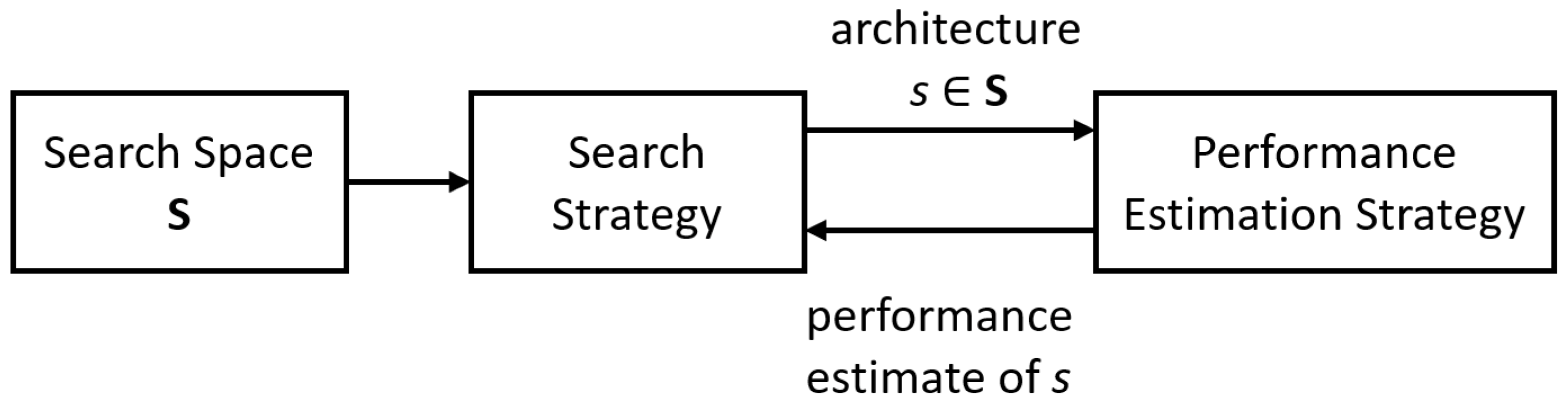
Following the exponential growth of computing power and availability of cloud computing resources in recent years, automated machine learning (AutoML) has received tremendous attention in both industry and academia. AutoML provides an attractive alternative to the manual ML practice as it promises to deliver high-performance end-to-end ML pipelines covering data preparation (cleaning and preprocessing), feature engineering (extraction, selection, and construction), model generation (selection and hyperparameter tuning), and model evaluation requiring minimal effort or intervention from the user [16,17,18]. AutoML services have become a standard offering in many technology companies, for example Cloud ML by Google and SageMaker by Amazon. Early work by Zoph et al. [19] highlighted the potential of AutoML in which a recurrent network was trained with reinforcement learning to automatically search for the best-performing architecture. Since then, research interest in AutoML has exploded, with a primary focus on neural architecture search (NAS), which seeks to construct well-performing neural architectures through the selection and combination of various basic modules from a predefined search space [16,20,21]. NAS algorithms can be categorised based on three dimensions: the search space, the search strategy, and the performance estimation strategy [20,21] (Figure 1). The search space defines the type of models that can be designed, this may include simple blocks or modules stacked on each other, or more complicated structures that include skipping connections and submodules. Common NAS structure types are entire structures [19,22], cell-based structures [23,24], progressive structures [25], and morphism-based structures [26,27]. As the search space is often exponentially large or even unbounded, a search strategy that typically consists of a hyperparameter optimisation algorithm such as Bayesian optimisation [17,28,29], evolutionary algorithm [30,31], reinforcement learning [19,32], or gradient descent [33] is used to explore the search space. Once an architecture is selected, it is evaluated using a performance estimation strategy, which speeds up performance evaluation through the use of either proxy metrics [24,34], extrapolation of performance via learning curve [35,36], or shortening of model training times by inheriting [30,37] or sharing weights [38,39,40] between architectures.
NAS-generated models have achieved SOTA performance and outperformed manually designed architectures on computer vision tasks such as image classification [41], object detection [42], and semantic segmentation [43]. However, despite AutoML showing great promise for computer vision tasks, to the best of our knowledge, no study has used AutoML for image-based plant phenotyping. To address this gap in knowledge, we examined the application of AutoML for image-based plant phenotyping using wheat lodging assessment with UAV imagery as an example. The performance of an open-source AutoML system, AutoKeras, was compared to transfer learning using pretrained CNN architectures on image classification and image regression tasks. For image classification, plot images were classified as either non-lodged or lodged; for image regression, lodged plot images were used as inputs to predict lodging scores. The merits and drawbacks of AutoML compared to transfer learning for image-based plant phenotyping are discussed. This study presents general methodology and workflows for the implementation of AutoKeras for image classification and regression applicable to the plant phenotyping task. In addition, specific methodology and workflows, including the use of a customised lodging score for UAV-based high-throughput wheat lodging assessment via AutoML and/or transfer learning are also provided.
2. Materials and Methods
2.1. Field Experiment
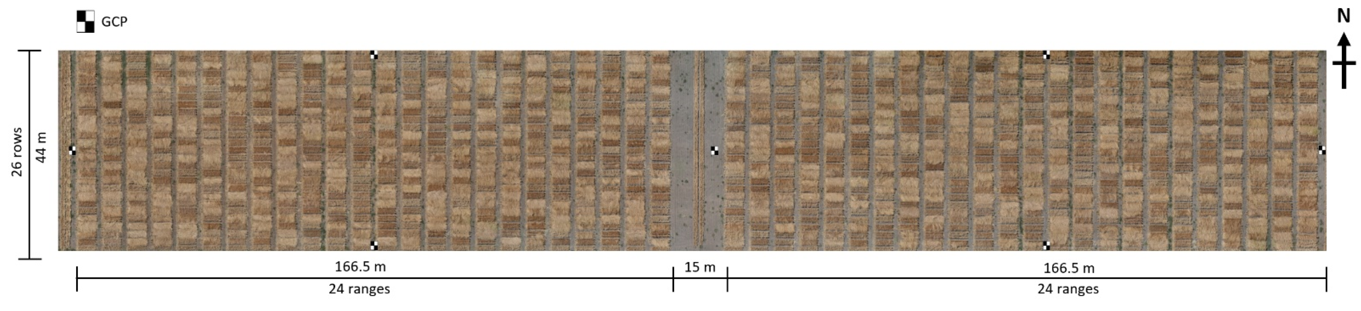
A wheat breeding experiment was conducted at Agriculture Victoria, Horsham, Australia during the winter–spring cropping season of 2018 (Lat: 36°44′35.21″ S Lon: 142°6′18.01″ E) (Figure 2). Seeds were sown to a planting density of 150 plants/m2 in individual plots measuring 5 m long and 1 m wide (5 m2), with a total of 1248 plots. Severe wind events towards the end of the cropping season (30th November–9th December) resulted in significant lodging of wheat plots across the experiment. Ground-truth labels for “lodged” and “non-lodged” were provided by an experienced field technician and a plant scientist.
2.2. Image Acquisition and Processing
High-resolution aerial imaging of wheat plots with different lodging grades was performed on 11 December 2018. Aerial imagery was acquired on a DJI Matrice M600 Pro (Shenzhen DJI Sciences and Technologies Ltd., Shenzhen, China) UAV with a Sony A7RIII RGB camera (35.9 mm × 24.0 mm sensor size, 42.4 megapixels resolution) mounted on a DJI Ronin MX gimbal. Flight planning and automatic mission control was performed using DJI’s iOS application Ground Station Pro (GS Pro). The camera was equipped with a 55 mm fixed focal length lens and set to 1 s interval shooting with JPEG format in shutter priority mode. Images were geotagged using a GeoSnap Express system (Field of View, Fargo, ND, USA). The flight mission was performed at an altitude of 45 m with front and side overlap of 75% under clear sky conditions. Seven black and white checkered square panels (38 cm × 38 cm) were distributed in the field experiment to serve as ground control points (GCPs) for the accurate geo-positioning of images (Figure 1). A real-time kinematic global positioning system (RTK-GPS) receiver, EMLID Reach RS (https://emlid.com, accessed on 28 January 2021) was used to record the centre of each panel with <1 cm accuracy.
Images were imported into Pix4Dmapper version 4.4.12 (Pix4D, Prilly, Switzerland) to generate an orthomosaic image, with the coordinates of the GCPs used for geo-rectification. The resulting orthomosaic had a ground sampling distance (GSD) of 0.32 cm/pixel. Individual plot images were clipped and saved in TIFF format from the orthomosaic using a field plot map with polygons corresponding to the experimental plot dimension of 5 m × 1 m in ArcGIS Pro version 2.5.1 (Esri, Redlands, CA, USA).
2.3. Lodging Assessment
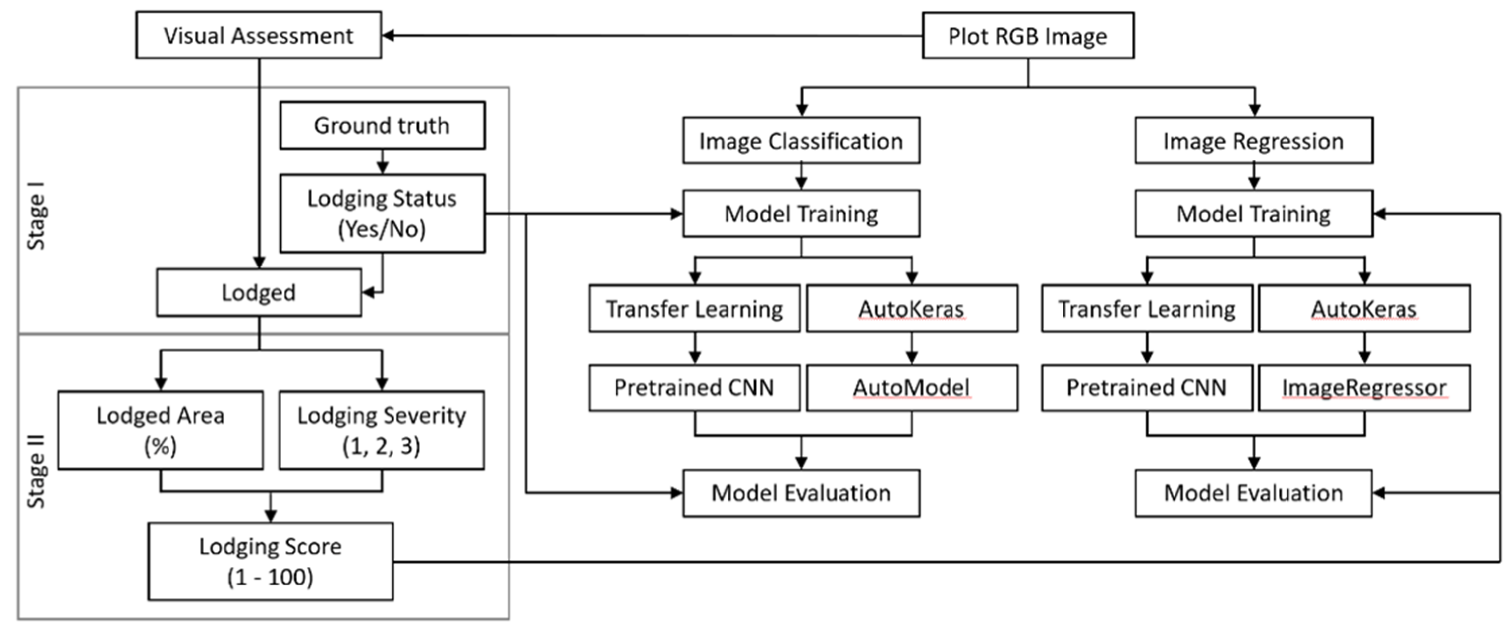
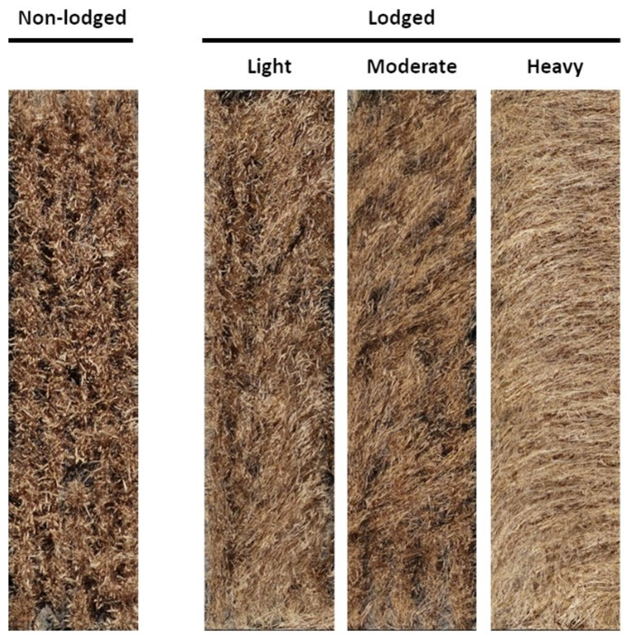
A two-stage assessment of lodging was performed in this study, and the results were used as the basis for image classification and image regression tasks (see Section 2.4) (Figure 3). The image classification task corresponded to the first stage of assessment in which the lodging status, i.e., whether the plot is lodged (yes) or non-lodged (no) was provided by the ground truth data and this could be verified easily from visual inspection of the high-resolution plot images (Figure 4). The image regression task corresponded to the second stage of assessment where plots identified as lodged were evaluated using a modified lodging score based on the method of Fischer and Stapper [44]:
Lodging severity values of 1 to 3 were assigned to three main grades of lodging based on the inclination angle between the wheat plant and the vertical line as follows: light lodging (severity 1; 10°–30°), moderate lodging (severity 2; 30°–60°), and heavy lodging (severity 3; 60°–90°) (Figure 3) [45]. The Lodged area (%) was determined visually from the plot images as the percentage of area lodged in the plot in proportion to the total plot area. The derived lodging score ranged between values of 1 and 100, with a score of 100 indicating that the entire plot was lodged with heavy lodging.
2.4. Deep Learning Experiments
Deep learning experiments were conducted in Python 3.7. The performance of the open-source AutoML framework, AutoKeras [28] version 1.0.1, in image classification and image regression was compared to that of a manual approach using transfer learning with pretrained modern CNN architectures implemented in Keras, Tensorflow-GPU version 2.1. For the image classification task, a binary classification scheme assigning individual plot images to either non-lodged (class 0) or lodged (class 1) was performed. For the image regression task, lodged plot images were used as inputs to predict the lodging score. Training and evaluation of the models were performed on an NVIDIA Titan RTX GPU (24 GB of GPU memory) at SmartSense iHub, Agriculture Victoria.
2.4.1. Training, Validation, and Test Datasets
For image classification, the image dataset consisted of 1248 plot images with 528 plots identified as non-lodged (class 0) and 720 plots identified as lodged (class 1). Images were first resized (downsampled) to the dimensions of 128 width × 128 height × 3 channels (Section 2.4.2) and these were split 80:20 (seed number = 123) into training (998 images) and test (250 images) datasets. For image regression, the 720 resized plot images identified as lodged were split 80:20 (seed number = 123) into training (576 images) and test (144 images) datasets. Images were fed directly into AutoKeras without preprocessing as this was done automatically by AutoKeras. In contrast, images were preprocessed to the format required by the corresponding pretrained CNN using the provided preprocess_input function in Keras. For model training on both image classification and regression, the training dataset was split further 80:20 (seed number = 456) into training and validation datasets. The validation dataset was used to evaluate training efficacy, with lower validation loss (as defined by the loss function, Section 2.4.2) indicating a better-trained model. Performance of trained models was evaluated on the test dataset (Section 2.4.4).
2.4.2. AutoML with AutoKeras
AutoKeras is an open-source AutoML framework built using Keras, which implements state-of-the-art NAS algorithms for computer vision and machine learning tasks [28]. It is also the only open-source NAS framework to offer both image classification and regression abilities at the time of this study. In our study, we experienced great difficulty in getting AutoKeras to stably complete experiments in default settings due to errors relating to graphics processing unit (GPU) memory usage and model tuning. This is not entirely unexpected as the beginning version 1.0, AutoKeras has undergone significant application programming interface (API) and system architecture redesign to incorporate KerasTuner ver. 1.0 and Tensorflow ver. 2.0. This change was necessary for AutoKeras to capitalise on recent developments in NAS and the DL framework, Tensorflow, in addition to providing support for the latest graphics processing unit (GPU) hardware. To partly circumvent the existing issues, we had to implement two approaches for the DL experiments to stably complete up to 100 trials, which is the number of models evaluated by AutoKeras (i.e., 100 trials = 100 models). Firstly, all images were resized to the dimensions of 128 × 128 × 3, and secondly, for image classification, we had to implement a custom image classifier using the provided AutoModel class in AutoKeras. We were not successful in completing experiments beyond 100 trials, and as such, only results up to 100 trials were presented in this study.
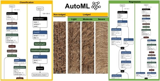
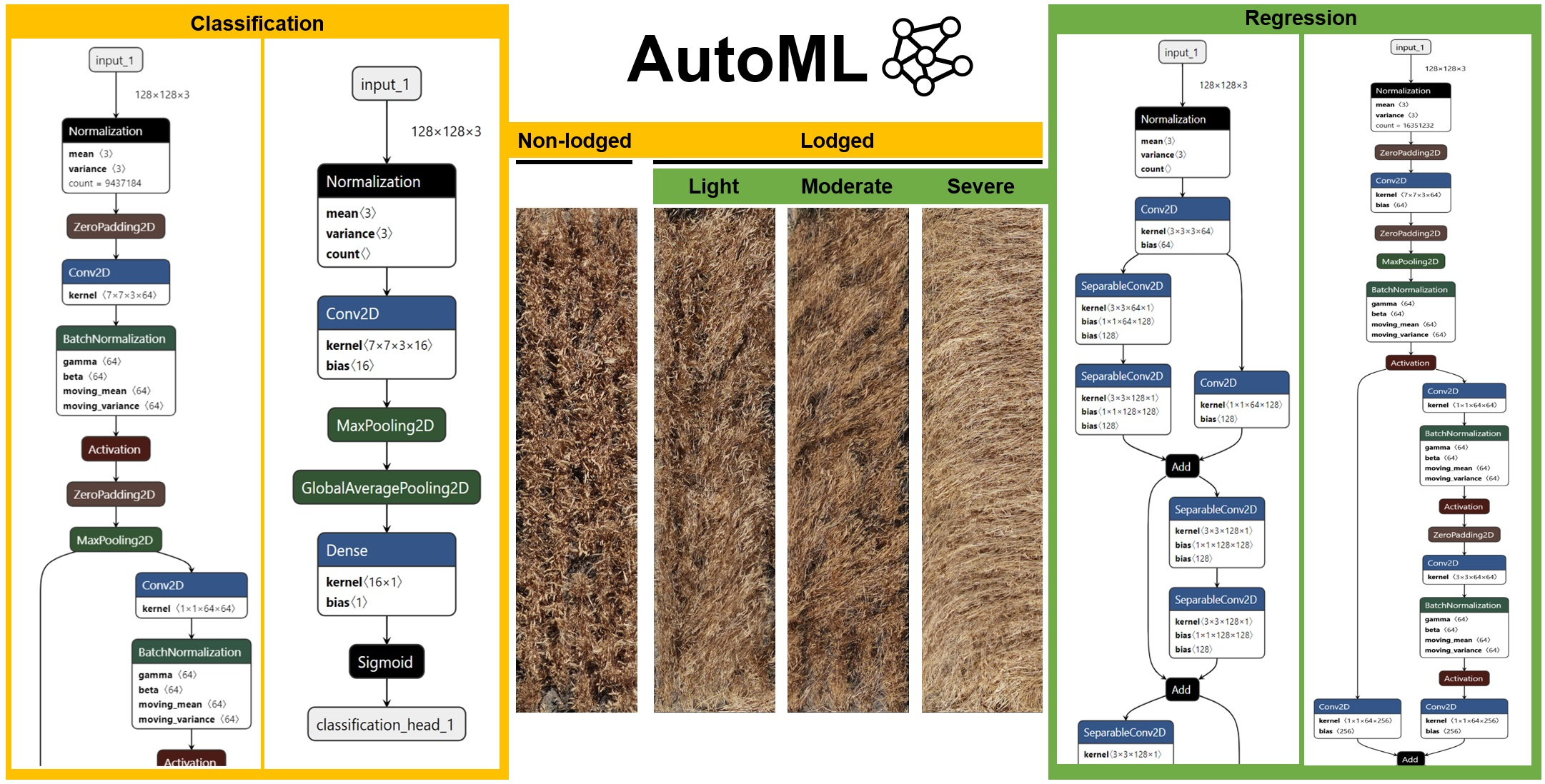
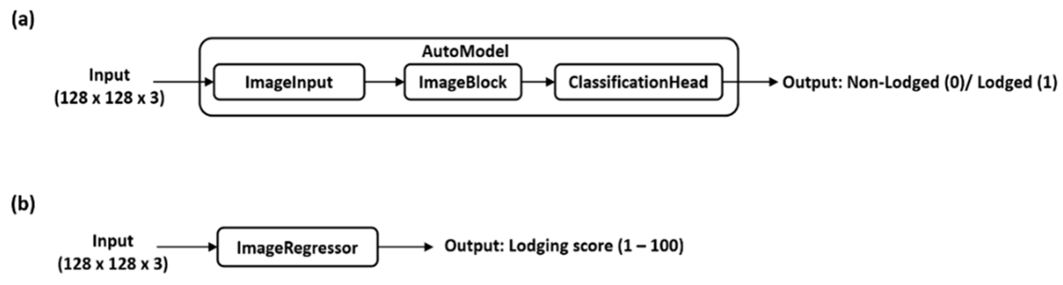
For image classification, a custom image classifier was defined using the AutoModel class, which allows the user to define a custom model by connecting modules/blocks in AutoKeras (Figure 5). In most cases, the user only needs to define the input node(s) and output head(s) of the AutoModel, as the rest is inferred by AutoModel itself. In our case, the input nodes were first an ImageInput class accepting image inputs (128 × 128 × 3), which in turn was connected to an ImageBlock class that selects iteratively from either a ResNet [46], ResNext [47], Xception [48], or simple CNN building blocks to construct neural networks of varying complexity and depth. The input nodes were joined to a single output head, the ClassificationHead class, which performed the binary classification (Figure 5a). The AutoModel was fitted to the training dataset with the tuner set as “Bayesian”, loss function as “binary_crossentropy”, evaluation metrics as “accuracy”, and 200 training epochs (rounds) for 10, 25, 50, and 100 trials with a seed number of 10. For image regression, the default AutoKeras image regression class, ImageRegressor, was fitted to the training dataset with the loss function as mean squared error (MSE), evaluation metrics as mean absolute error (MAE), and mean absolute percentage error (MAPE), and 200 training epochs for 10, 25, 50, and 100 trials with a seed number of 45 (Figure 5b).
The performances of the best models from 10, 25, 50, and 100 trials were evaluated on their respective test datasets (Section 2.4.4) and exported as Keras models to allow neural network visualisation using the Netron software (https://github.com/lutzroeder/netron, accessed on 28 January 2021).
2.4.3. Transfer Learning with Pretrained CNNs
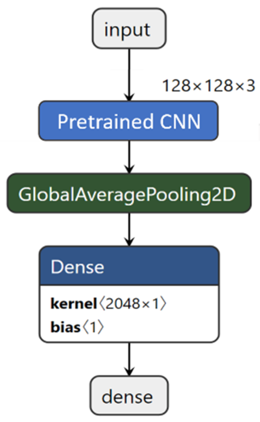
Transfer learning is a popular approach in DL, where a pretrained model is reused as the starting point for a model on a second task [4]. This allows the user to rapidly deploy complex neural networks, including state-of-the-art DL architectures without incurring time and computing costs. In this study, transfer learning was performed using VGG networks [49], residual networks (ResNets) [46], InceptionV3 [50], Xception [48], and densely connected CNNs (DenseNets) [51] pretrained on the ImageNet dataset. These networks were implemented in Keras as a base model using the provided Keras API with the following parameters: weights = “imagenet”, include_top = False and input_shape = (128, 128, 3) (Figure 6). Output from the base model was joined to a global average pooling 2D layer and connected to a final dense layer, with the activation function set as either “sigmoid” for image classification or “linear” for image regression. The model was compiled with the batch size as 32, optimiser as “Adam”, and corresponding loss functions and evaluation metrics as described in Section 2.4.2. Model training occurred in two stages for both image classification and regression tasks: in the first stage (100 epochs), weights of the pretrained layers were frozen, and the Adam optimiser had a higher learning rate (1 × 10⁻¹ or 1 × 10⁻²) to allow faster training of the top layers; in the second stage (200 epochs), weights of the pretrained layers were unfrozen, and the Adam optimiser had a smaller learning rate (1 × 10⁻² to 1 × 10⁻⁵) to allow fine-tuning of the model. Learning rates were optimised for each CNN and the values that provided the best model performance are provided in Table 1. Performance of the trained models was evaluated on their respective test datasets (Section 2.4.4).
2.4.4. Model Evaluation Metrics
For image classification, model performance on the test dataset was evaluated using classification accuracy and Cohen’s kappa coefficient [52]. For image regression, in addition to the mean absolute error (MAE) and the mean absolute percentage error (MAPE) provided by AutoKeras and Keras, the coefficient of determination (R2) and the root mean-squared error (RMSE) were also calculated to determine model performance on the test dataset. Models were also evaluated based on total model training time (in minutes, min) and inference time on the test dataset presented as mean ± standard deviation per image in milliseconds (ms).
- Accuracy: accuracy represents the proportion of correctly predicted data points over all data points. It is the most common way to evaluate a classification model and works well when the dataset is balanced.where tp = true positives, fp = false positives, tn = true negatives, and fn = false negatives.
- Cohen’s kappa coefficient: Cohen’s kappa () expresses the level of agreement between two annotators, which in this case, is the classifier and the human operator on a classification problem. The kappa score ranges between −1 to 1, with scores above 0.8 generally considered good agreement.where is the empirical probability of agreement on the label assigned to any sample (the observed agreement ratio), and is the expected agreement when both annotators assign labels randomly.
- Root mean-squared error (RMSE): root mean-squared error provides an idea of how much error a model typically makes in its prediction, with a higher weight for large errors. As such, RMSE is sensitive to outliers, and other performance metrics may be more suitable when there are many outlier districts.where … are predicted values, … are observed values, and n is the number of observations.
- Mean absolute error (MAE): mean absolute error, also called the average absolute deviation is another common metric used to measure prediction errors in a model by taking the sum of absolute value of error. Compared to RMSE, MAE gives equal weight to all errors and as such may be less sensitive to the effects of outliers.where … are predicted values, … are observed values, and n is the number of observations.
- Mean absolute percentage error (MAPE): mean absolute percentage error is the percentage equivalent of MAE, with the errors scaled against the observed values. MAPE may be less sensitive to the effects of outliers compared to RMSE but is biased towards predictions that are systematically less than the actual values due to the effects of scaling.where … are predicted values, … are observed values, and n is the number of observations.
- Coefficient of determination (R2): the coefficient of determination is a value between 0 and 1 that measures how well a regression line fits the data. It can be interpreted as the proportion of variance in the independent variable that can be explained by the model.where … are predicted values, … are observed values, is the mean of observed values, and n is the number of observations.
3. Results
3.1. Image Classification
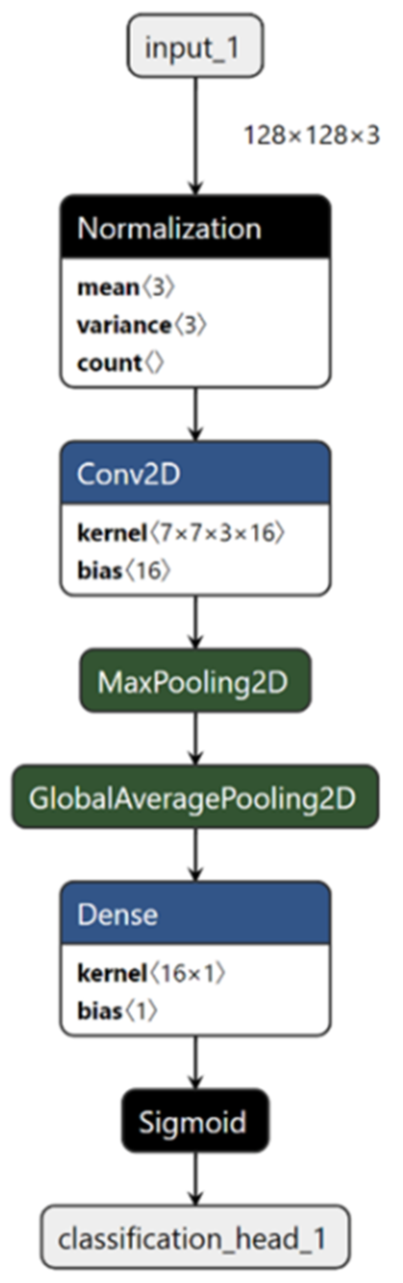
Both transfer learning with pretrained CNNs and AutoKeras performed strongly in the image classification task (Table 2). Transfer learning’s performance with pretrained CNNs ranged from 91.6% to 93.2% classification accuracy, with Xception (accuracy = 93.2%, kappa = 0.8612) and DenseNet-201 (accuracy = 93.2%, kappa = 0.8599) giving the best overall accuracy (Table 2). Among the pretrained CNNs, InceptionV3 had the fastest training (5.42 min) and inference (0.4022 ± 0.0603 ms per image) times, whereas DenseNet-201 had the slowest training (11.79 min) and inference (0.7524 ± 0.0568 ms per image) times. In comparison, AutoKeras’ (AK) performance ranged from 86.8% to 92.4% accuracy, with performance improving as more models (trials) were evaluated (Table 2). The best AutoKeras model was discovered from 100 trials and had the same 92.4% accuracy as the ResNet-50 (Table 2). Impressively, AutoKeras was able to achieve this result using a simple two-layer CNN (43,859 parameters) consisting only of a single 2D convolutional layer (Figure 7) as opposed to the 50-layer deep ResNet-50 architecture (~23.6 million parameters). The two-layer CNN had the fastest overall inference time (0.0228 ± 0.0005 ms per image) on the test dataset compared to other models, which was ~18-fold faster compared to the InceptionV3 and up to ~33-fold faster compared to the DenseNet-201 (Table 2). However, model training times for AutoKeras were significantly higher compared to those of the transfer learning approaches, with the longest training time of 251 min recorded for 100 trials, which was ~21-fold higher compared to the DenseNet-201 (Table 2). Confusion matrices of the test set for the best models from transfer learning and AutoML for image classification are presented in Table 3. Examination of the model architectures returned by AutoKeras revealed that the best model architecture resulting from the 10 and 25 trials was a deep CNN model comparable in depth and complexity to the ResNet-50 (Supplementary Figure S1), highlighting the ability of AutoKeras to explore deep CNN architectures even in a small model search space. Subsequently, when the model search space was extended to 50 and 100 trials, the best model architecture discovered by AutoKeras was the two-layer CNN model (Figure 7).
3.2. Image Regression
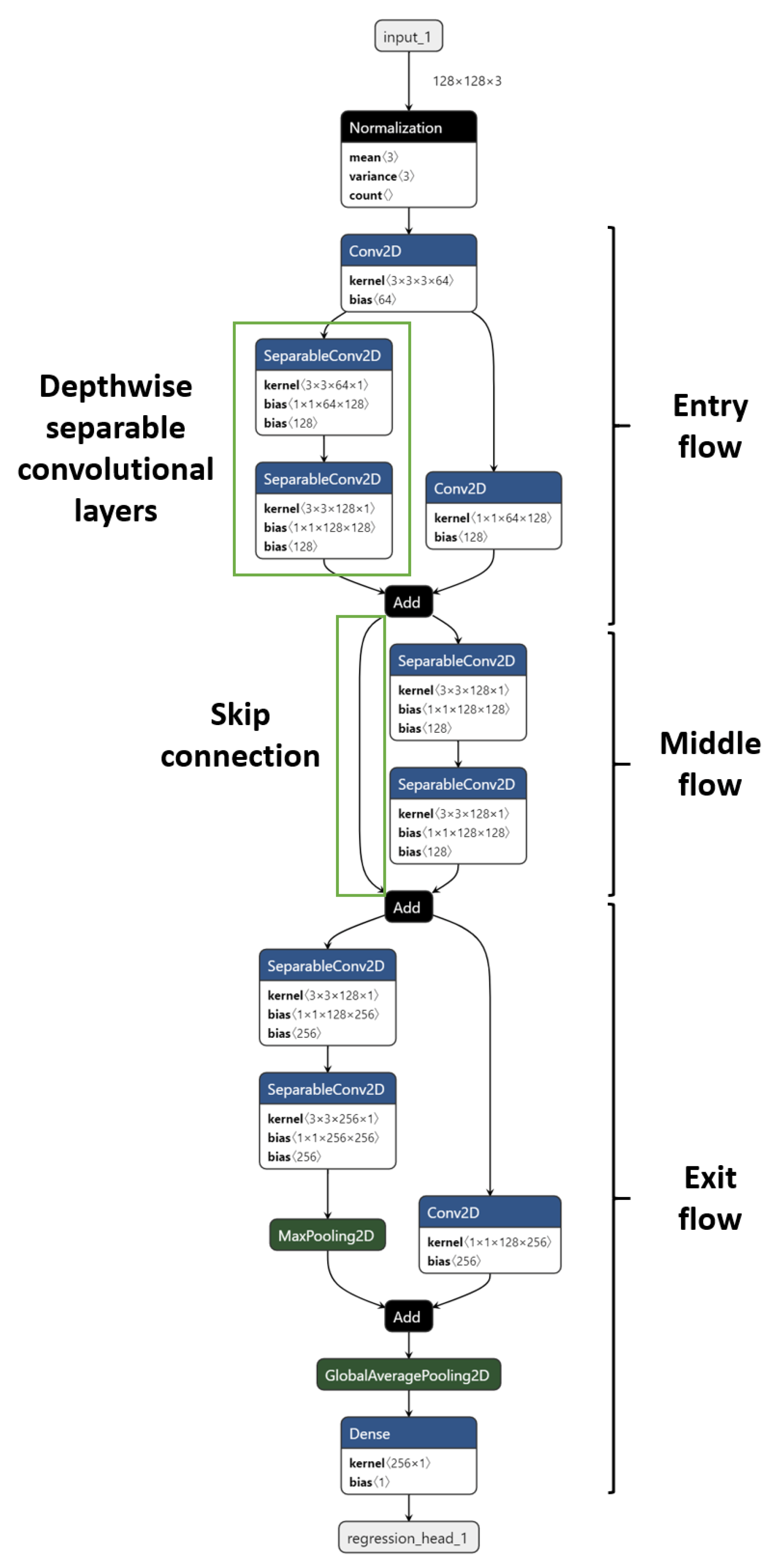
For the image regression task, transfer learning with DenseNet-201 gave the best overall performance (R2 = 0.8303, RMSE = 9.55, MAE = 7.03, MAPE = 12.54%), followed closely by AutoKeras (AK) with the model from 100 trials (R2 = 0.8273, RMSE = 10.65, MAE = 8.24, MAPE = 13.87%) (Table 4). The CNN models varied in regression performance, with R2 ranging between 0.76 and 0.83. Within the pretrained CNNs, DenseNet-201 had the slowest model training (7.01 min) and per image inference (0.8141 ± 0.1059 ms) times, with ResNet-50 having the fastest training (3.55 min) time, with a per image inference time of 0.5502 ± 0.0716 ms. For AutoKeras, performance generally improved from 10 to 100 trials (Table 4). AutoKeras was able to achieve the second-best performance using an eight-layer CNN resembling a truncated mini Xception network with 207,560 total parameters (Figure 8). Two prominent features of the original 71-layer deep Xception network, namely the use of depthwise separable convolution layers and skip connections were evident in the AutoKeras model (Figure 8). Notably, the mini Xception network outperformed the original pretrained Xception network (R2 = 0.7709, RMSE = 11.08, MAE = 8.22, MAPE = 13.51%) (Table 4). Not surprisingly, the mini Xception network had the fastest per image inference time (0.0199 ± 0.0008 ms) compared to the other models, which was ~27-fold faster compared to the ResNet-50 and up to 41-fold faster compared to the DenseNet-201 (Table 4). However, model training times for AutoKeras was again significantly higher compared to the transfer learning approaches, with the longest training time of 325 min recorded for 100 trials, which was ~46 fold higher compared to the DenseNet-201 (Table 4). Examination of the model architectures returned by AutoKeras revealed that the best model architecture resulting from the 10 and 25 trials was a deep CNN model (Supplementary Figure S2), whereas the best model architecture discovered from 50 and 100 trials was the eight-layer mini Xception model (Figure 8).
4. Discussion
Using wheat lodging assessment as an example, we compared the performance of an open-source AutoML framework, AutoKeras, to transfer learning using modern CNN architectures for image classification and image regression. As a testament to the power and efficacy of modern DL architectures for computer vision tasks, both AutoKeras and transfer learning approaches performed well in this study, with transfer learning exhibiting a slight performance advantage over AutoKeras.
For the image classification task, plot images were classified as either non-lodged or lodged. The best classification performance of 93.2% was jointly achieved by transfer learning with Xception and DenseNet-201 networks. This is not entirely surprising as both Xception [48] and DenseNet [51] were developed later as improved architectures compared to the other CNNs in this study. In contrast, the best AutoKeras model (from 100 trials) achieved an accuracy of 92.4%, which is the same as those obtained by transfer learning with ResNet-50. Classification results in this study are comparable to those reported in a smaller study which classified 465 UAV-acquired wheat plot multispectral images (red, green, blue channels used in models) as either non-lodged/lodged with a hand-crafted deep neural network, LodgedNet (97.7% accuracy) and other modern DL networks (97.7–100.0% accuracies) via transfer learning [53]. The higher classification accuracies reported in that study may be due to the use of image data augmentation (i.e., increasing training dataset via image transformations) which generally improves model performance and that images were acquired prematurity (plants were still green) allowing variations in colour to potentially contribute more informative features for modelling [45,53]. Results in our study suggest that NAS-generated models can provide competitive performance compared to modern, human-designed CNN architectures, with transfer learning using pretrained CNNs exhibiting a slight performance advantage (~1% improvement) over AutoML models. A recent survey comparing the performance of manually designed models against those generated by NAS algorithms on the CIFAR-10 dataset, a public dataset commonly used for benchmarking in image classification, found that the top two best-performing models were both manually designed models [16]. However, the gap between the manual and AutoML models was very small (<1% accuracy difference). In our study, AutoKeras was able to achieve results comparable to those of the 50-layer deep ResNet-50 model (~25 million parameters) using only a simple two-layer CNN model (43,859 parameters). The two-layer CNN had the fastest inference time (0.0228 ± 0.0005 ms per image) compared to the other models, which was up to 33-fold faster compared to the DenseNet-201, which had the slowest inference time. As such, the two-layer CNN could prove useful for real-time inferencing, although its simple or shallow architecture raises concern about its generalisability across different datasets. This can be addressed in future studies by using datasets derived from multiple trials or imaging conditions for AutoML training to obtain a solution generalised across different environments.
For the image regression task, lodged plot images were used as inputs to predict the lodging score. The best performance (R2 = 0.8303, RMSE = 9.55, MAE = 7.03, MAPE = 12.54%) was obtained using transfer learning with DenseNet-201, followed closely by AutoKeras (R2 = 0.8273, RMSE = 10.65, MAE = 8.24, MAPE = 13.87%) with the model discovered from 100 trials. In both image classification and regression tasks, transfer learning with DenseNet-201 achieved the best results. DenseNet can be considered as an evolved version of the ResNet [46], where the outputs of the previous layers are merged via concatenation with succeeding layers to form blocks of densely connected layers [51]. However, similarly for image classification, the DenseNet-201 had the slowest inference time (117.23 ± 15.25 ms) on the test dataset in image regression, making it less suitable for time-critical applications such as real-time inferencing. In comparison, the AutoKeras model resembled a mini eight-layer Xception model (207,560 parameters) and had the fastest inference time (0.0199 ± 0.0008 ms per image) on the test dataset, which was ~41-fold faster compared to the DenseNet-201. In its original form, the Xception network is 71 layers deep (~23 million parameters) and consists of three parts: the entry flow, middle flow, and exit flow [48]. These three parts and two key features of the Xception network, namely the depthwise separable convolutions and skip connections originally proposed in ResNet, were discernible from the mini Xception model. Research in the area of network pruning, which compresses deep neural network through the removal/pruning of redundant parameters showed that it is possible to have equally performant models with up to 97% of the parameters pruned [54]. Although dissimilar to network pruning, as evidenced in our study, AutoKeras can discover efficient and compact model architectures through the NAS process. However, NAS-generated models are typically limited to variants or combinations of modules derived from existing, human-designed CNN architectures [16,20,21]; although recent innovations in NAS have uncovered novel CNN architectures such as SpineNet for object detection [55].
The lodging score originally proposed by Fischer and Stapper [44] is calculated from the lodging angle and lodged area (lodging score = angle of lodging from vertical position/90 × % lodged area). In our study, the angle of lodging is replaced by lodging severity, which is a score of 1 to 3 assigned to light, moderate, and heavy lodging grades as determined by visual assessment of lodged plot images. Consequently, under- or overestimation of lodging scores may happen for plots within the same lodging severity grade. For example, plots with 100% lodged area and lodging angle of 65° (lodging severity 3) and 90° (lodging severity 3) will have the same lodging score of 100 in this study as opposed to scores of 72 and 100 according to the original method. This may partly account for the model prediction errors in the image regression task. Nonetheless, the modified lodging score allowed a rapid evaluation of wheat lodging based on visual assessments of UAV imagery and was useful as a target for image regression. For detailed assessment of lodging and model performance in lodging score prediction, future studies should incorporate manual ground-truthing of the lodging angle and lodged area to enable a more accurate calculation of lodging scores. The current AutoML and transfer learning workflows presented for wheat lodging assessment based on UAV imagery have the potential to replace manual observations, which are time-consuming and prone to human error. However, further research and data are required to train and validate a robust model applicable across different field environments, including at various crop growth stages.
One of the challenges in this study was getting AutoKeras to perform stably and complete the DL experiments. Initial attempts were often met with an out of memory (OOM) error message, arising from AutoKeras trying to load models too large to fit in the GPU memory. Prior to version 1.0, AutoKeras had a GPU memory adaptation function that limits the size of neural networks according to the GPU memory [28]. However, beginning with version 1.0, this function is no longer implemented in AutoKeras (personal communication with Haifeng Jin, author of AutoKeras) and may partially account for the OOM errors. To partly circumvent this issue, we had to resize all input images (1544 × 371) to a smaller size of 128 × 128, which allowed AutoKeras to complete experiments up to 100 trials. The impact of the downsized images on AutoKeras model performance would need to be ascertained in future studies, although the 128 × 128 image size is within common ranges observed in DL models, for example, LodgedNet (64 × 128) [53] and established modern CNN architectures (224 × 224) [46,49,51]. As AutoKeras is undergoing active development, we are hopeful that issues encountered in our study will be resolved in future releases. It will be interesting to explore AutoKeras’ performance with larger model search space (>100 trials) using higher-resolution input images coupled with image data augmentation where appropriate in future studies.
Transfer learning using existing modern CNN architectures achieved better results compared to AutoML in both image classification and regression tasks in this study. However, a major limitation is that these CNN models have been trained using three-channel RGB images and this prevents direct application of these models for image sources beyond three channels, such as multispectral and hyperspectral images [53]. In addition, existing CNN architectures may not always provide the best performance compared to custom-designed models. However, modification of existing CNN architectures or manually designing CNN models are time-consuming and technically challenging. In this regard, AutoML provides an attractive alternative as it can deliver CNN models with good performance out-of-the-box and can accept inputs of varying sizes and dimensions, making it ideal for use on diverse sensor-derived data including multispectral and hyperspectral imagery. Furthermore, an added benefit of AutoML is its potential through NAS to discover compact model architectures that are ideal for real-time inferencing. However, to ensure generalisability of the NAS-generated models across datasets, it is vital to use a training dataset representative of the diverse trial environments and imaging conditions in future studies. At first glance, a downside of AutoML appears to be the long training times (hours as opposed to minutes) required to achieve models with competitive performance compared to transfer learning, even when using modern GPU hardware. However, model training times alone do not provide a complete picture of the total experimental or operational time (including manual hours) spent on each of the approaches. For example, transfer learning in this study entailed countless man-hours necessary to select, compare, and fine-tune pretrained CNN models. In that regard, the hours incurred in AutoML would not differ much and may even compare favourably to the total operational time spent on transfer learning. The significant GPU computational costs associated with AutoML hinder it from being widely adopted by DL practitioners for now. However, this is expected to be offset in time by the rapid growth in GPU computing power and the concurrent rise in GPU affordability. Another concern relating to AutoML is the reproducibility of results owing to the stochastic nature of NAS [56]. This concern can largely be addressed through making available all datasets, source codes (including exact seeds used), and best models reported in the NAS study—a practice embraced in this study (see Data Availability).
5. Conclusions
Results in our study demonstrate that transfer learning with modern CNNs performed better compared to AutoML, although the performance differences were minimal, and the current AutoML performance observed may not be at its full potential due to technical issues. For most computer vision tasks using RGB image datasets, transfer learning with existing CNNs will provide a good starting point and should yield satisfactory results in most cases with minimal effort and time. However, for plant phenotyping applications that are time critical and generate image datasets beyond the standard RGB three channels, AutoML is a good alternative to manual DL approaches and should be in the toolbox of both novice and expert users alike. For field-based crop phenotyping, portable multispectral and hyperspectral sensors are becoming common on ground-based and aerial HTP platforms [3], providing ample avenues for AutoML application. Moving forward, with the exponential rise in GPU computing power and strong interests in NAS research, AutoML systems are expected to become more ubiquitous. In tandem with existing DL practices, they can contribute significantly towards the streamlined development of image analytical pipelines for HTP systems integral to improving breeding program and crop management efficiencies. Results in our study provide a basis for the adoption and application of AutoML systems for high-throughput image-based plant phenotyping.
Supplementary Materials
The following are available online at https://www.mdpi.com/2072-4292/13/5/858/s1, Figure S1: Best AutoKeras model architecture discovered from 10 and 25 trials for image classification, Figure S2: Best AutoKeras model architecture discovered from 10 and 25 trials for image regression.
Author Contributions
Conceptualisation, J.C.O.K., G.S., and S.K.; methodology, software, validation, formal analysis, data curation, and writing—original draft preparation, J.C.O.K.; investigation, resources, writing—review and editing, and supervision, S.K.; project administration and funding acquisition, S.K. and G.S. All authors have read and agreed to the published version of the manuscript.
Funding
This research received no external funding.
Data Availability Statement
Datasets containing 1248 digital images (1544 × 371 pixels) of individual wheat plots with varying grades of lodging and corresponding lodging data are available on Zenodo [57]. Ground-truth data for lodging status and calculated lodging scores are provided as a comma-separated values (CSV) file. Source codes required to replicate the analyses in this article and the best performing models reported for AutoKeras are provided in a GitHub repository [58].
Acknowledgments
We thank Dennis Ward and Emily Thoday-Kennedy for technical support in conducting the field experiment.
Conflicts of Interest
The authors declare no conflict of interest.
References
- Ninomiya, S.; Baret, F.; Cheng, Z.-M.M. Plant Phenomics: Emerging Transdisciplinary Science. Plant Phenom. 2019, 2019, 1–3. [Google Scholar] [CrossRef] [PubMed]
- Tardieu, F.; Cabrera-Bosquet, L.; Pridmore, T.; Bennett, M. Plant Phenomics, From Sensors to Knowledge. Curr. Biol. 2017, 27, R770–R783. [Google Scholar] [CrossRef] [PubMed]
- Mir, R.R.; Reynolds, M.; Pinto, F.; Khan, M.A.; Bhat, M.A. High-throughput phenotyping for crop improvement in the genomics era. Plant Sci. 2019, 282, 60–72. [Google Scholar] [CrossRef] [PubMed]
- Jiang, Y.; Li, C. Convolutional Neural Networks for Image-Based High-Throughput Plant Phenotyping: A Review. Plant Phenom. 2020, 2020, 1–22. [Google Scholar] [CrossRef] [Green Version]
- Chen, M.; Tang, Y.; Zou, X.; Huang, K.; Huang, Z.; Zhou, H.; Wang, C.; Lian, G. Three-dimensional perception of orchard banana central stock enhanced by adaptive multi-vision technology. Comput. Electron. Agric. 2020, 174, 105508. [Google Scholar] [CrossRef]
- Fu, L.; Gao, F.; Wu, J.; Li, R.; Karkee, M.; Zhang, Q. Application of consumer RGB-D cameras for fruit detection and localization in field: A critical review. Comput. Electron. Agric. 2020, 177, 105687. [Google Scholar] [CrossRef]
- Khan, A.; Sohail, A.; Zahoora, U.; Qureshi, A.S. A survey of the recent architectures of deep convolutional neural networks. Artif. Intell. Rev. 2020, 53, 5455–5516. [Google Scholar] [CrossRef] [Green Version]
- Minaee, S.; Boykov, Y.Y.; Porikli, F.; Plaza, A.J.; Kehtarnavaz, N.; Terzopoulos, D. Image Segmentation Using Deep Learning: A Survey. IEEE Trans. Pattern Anal. Mach. Intell. 2021. [Google Scholar] [CrossRef] [PubMed]
- Wu, X.; Sahoo, D.; Hoi, S.C.H. Recent advances in deep learning for object detection. Neurocomputing 2020, 396, 39–64. [Google Scholar] [CrossRef] [Green Version]
- Balasubramanian, V.N.; Guo, W.; Chandra, A.L.; Desai, S.V. Computer Vision with Deep Learning for Plant Phenotyping in Agriculture: A Survey. Adv. Comput. Commun. 2020. Epub ahead of printing. [Google Scholar] [CrossRef]
- Watt, M.; Fiorani, F.; Usadel, B.; Rascher, U.; Muller, O.; Schurr, U. Phenotyping: New Windows into the Plant for Breeders. Annu. Rev. Plant Biol. 2020, 71, 689–712. [Google Scholar] [CrossRef] [PubMed]
- Tang, Y.; Chen, M.; Wang, C.; Luo, L.; Li, J.; Lian, G.; Zou, X. Recognition and Localization Methods for Vision-Based Fruit Picking Robots: A Review. Front. Plant Sci. 2020, 11, 510. [Google Scholar] [CrossRef] [PubMed]
- Chen, Y.; Lee, W.S.; Gan, H.; Peres, N.; Fraisse, C.; Zhang, Y.; He, Y. Strawberry Yield Prediction Based on a Deep Neural Network Using High-Resolution Aerial Orthoimages. Remote Sens. 2019, 11, 1584. [Google Scholar] [CrossRef] [Green Version]
- Fu, L.; Majeed, Y.; Zhang, X.; Karkee, M.; Zhang, Q. Faster R–CNN-based apple detection in dense-foliage fruiting-wall trees using RGB and depth features for robotic harvesting. Biosyst. Eng. 2020, 197, 245–256. [Google Scholar] [CrossRef]
- Chen, S.; Tang, M.; Kan, J. Predicting Depth from Single RGB Images with Pyramidal Three-Streamed Networks. Sensors 2019, 19, 667. [Google Scholar] [CrossRef] [Green Version]
- He, X.; Zhao, K.; Chu, X. AutoML: A survey of the state-of-the-art. Knowl. Based Syst. 2021, 212, 106622. [Google Scholar] [CrossRef]
- Truong, A.; Walters, A.; Goodsitt, J.; Hines, K.; Bruss, C.B.; Farivar, R. Towards Automated Machine Learning: Evaluation and Comparison of AutoML Approaches and Tools. In Proceedings of the 31st International Conference on Tools with Artificial Intelligence (ICTAI), Portland, OR, USA, 4–6 November 2019; IEEE: Piscataway, NJ, USA, 2019; pp. 1471–1479. [Google Scholar]
- Zöller, M.-A.; Huber, M.F. Benchmark and Survey of Automated Machine Learning Frameworks. J. Artif. Intell. Res. 2021, 70, 409–472. [Google Scholar] [CrossRef]
- Zoph, B.; Le, Q.V. Neural Architecture Search with Reinforcement Learning. arXiv 2016, arXiv:1611.01578. [Google Scholar]
- Elsken, T.; Metzen, J.H.; Hutter, F. Neural Architecture Search: A Survey. arXiv 2019, arXiv:1808.05377. [Google Scholar]
- Wistuba, M.; Rawat, A.; Pedapati, T. A Survey on Neural Architecture Search. arXiv 2019, arXiv:1905.01392. [Google Scholar]
- Pham, H.; Guan, M.; Zoph, B.; Le, Q.; Dean, J. Efficient Neural Architecture Search via Parameters Sharing. In Proceedings of the 35th International Conference on Machine Learning, Stockholm, Sweden, 10–15 July 2018; pp. 4095–4104. [Google Scholar]
- Zhong, Z.; Yan, J.; Liu, C. Practical Network Blocks Design with Q-Learning. arXiv 2017, arXiv:1708.05552. [Google Scholar]
- Zoph, B.; Vasudevan, V.; Shlens, J.; Le, Q.V. Learning Transferable Architectures for Scalable Image Recognition. In Proceedings of the 2018 IEEE/CVF Conference on Computer Vision and Pattern Recognition, Salt Lake City, UT, USA, 18–22 June 2018; IEEE: Piscataway, NJ, USA, 2018; pp. 8697–8710. [Google Scholar]
- Liu, H.; Simonyan, K.; Vinyals, O.; Fernando, C.; Kavukcuoglu, K. Hierarchical Representations for Efficient Architecture Search. arXiv 2018, arXiv:1711.00436. [Google Scholar]
- Chen, T.; Goodfellow, I.J.; Shlens, J. Net2Net: Accelerating Learning via Knowledge Transfer. arXiv 2016, arXiv:1511.05641. [Google Scholar]
- Wei, T.; Wang, C.; Rui, Y.; Chen, C.W. Network Morphism. In Proceedings of the 33rd International Conference on Machine Learning, New York, NY, USA, 20–22 June 2016; pp. 564–572. [Google Scholar]
- Jin, H.; Song, Q.; Hu, X. Auto-Keras: An Efficient Neural Architecture Search System. In Proceedings of the 25th ACM SIGKDD International Conference on Knowledge Discovery & Data Mining, Anchorage, AK, USA, 3–7 August 2019; Association for Computing Machinery: New York, NY, USA, 2019; pp. 1946–1956. [Google Scholar]
- Mendoza, H.; Klein, A.; Feurer, M.; Springenberg, J.T.; Urban, M.; Burkart, M.; Dippel, M.; Lindauer, M.; Hutter, F. Towards Automatically-Tuned Deep Neural Networks. In Automated Machine Learning: Methods, Systems, Challenges; Hutter, F., Kotthoff, L., Vanschoren, J., Eds.; Springer International Publishing: Cham, Switzerland, 2019; pp. 135–149. [Google Scholar] [CrossRef] [Green Version]
- Real, E.; Moore, S.; Selle, A.; Saxena, S.; Suematsu, Y.L.; Tan, J.; Le, Q.V.; Kurakin, A. Large-Scale Evolution of Image Classifiers. arXiv 2017, arXiv:1703.01041. [Google Scholar]
- Stanley, K.O.; Miikkulainen, R. Evolving Neural Networks through Augmenting Topologies. Evol. Comput. 2002, 10, 99–127. [Google Scholar] [CrossRef]
- Baker, B.; Gupta, O.; Naik, N.; Raskar, R. Designing Neural Network Architectures using Reinforcement Learning. arXiv 2017, arXiv:1611.02167. [Google Scholar]
- Liu, H.; Simonyan, K.; Yang, Y. DARTS: Differentiable Architecture Search. arXiv 2019, arXiv:1806.09055. [Google Scholar]
- Zela, A.; Klein, A.; Falkner, S.; Hutter, F. Towards Automated Deep Learning: Efficient Joint Neural Architecture and Hyperparameter Search. arXiv 2018, arXiv:1807.06906. [Google Scholar]
- Klein, A.; Falkner, S.; Springenberg, J.T.; Hutter, F. Learning Curve Prediction with Bayesian Neural Networks. In Proceedings of the 5th International Conference on Learning Representations (ICRL 2017), Toulon, France, 24–26 April 2017. [Google Scholar]
- Swersky, K.; Snoek, J.; Adams, R. Freeze-Thaw Bayesian Optimization. arXiv 2014, arXiv:1406.3896. [Google Scholar]
- Elsken, T.; Metzen, J.H.; Hutter, F. Efficient Multi-Objective Neural Architecture Search via Lamarckian Evolution. arXiv 2019, arXiv:1804.09081. [Google Scholar]
- Bender, G.; Kindermans, P.; Zoph, B.; Vasudevan, V.; Le, Q.V. Understanding and Simplifying One-Shot Architecture Search. In Proceedings of the 35th International Conference on Machine Learning, Stockholm, Sweden, 10–15 July 2018. [Google Scholar]
- Cai, H.; Zhu, L.; Han, S. ProxylessNAS: Direct Neural Architecture Search on Target Task and Hardware. arXiv 2019, arXiv:1812.00332. [Google Scholar]
- Xie, S.; Zheng, H.; Liu, C.; Lin, L. SNAS: Stochastic Neural Architecture Search. arXiv 2019, arXiv:1812.09926. [Google Scholar]
- Tan, M.; Le, Q.V. Efficientnet: Rethinking model scaling for convolutional neural networks. arXiv 2019, arXiv:1905.11946. [Google Scholar]
- Wang, N.; Gao, Y.; Chen, H.; Wang, P.; Tian, Z.; Shen, C.; Zhang, Y. NAS-FCOS: Fast Neural Architecture Search for Object Detection. In Proceedings of the 2020 IEEE/CVF Conference on Computer Vision and Pattern Recognition (CVPR), Seattle, WA, USA, 14–19 June 2020; IEEE: Piscataway, NJ, USA, 2020; pp. 11940–11948. [Google Scholar]
- Weng, Y.; Zhou, T.; Li, Y.; Qiu, X. NAS-Unet: Neural Architecture Search for Medical Image Segmentation. IEEE Access 2019, 7, 44247–44257. [Google Scholar] [CrossRef]
- Fischer, R.A.; Stapper, M. Lodging effects on high-yielding crops of irrigated semidwarf wheat. Field Crops Res. 1987, 17, 245–258. [Google Scholar] [CrossRef]
- Sun, Q.; Sun, L.; Shu, M.; Gu, X.; Yang, G.; Zhou, L. Monitoring Maize Lodging Grades via Unmanned Aerial Vehicle Multispectral Image. Plant Phenom. 2019, 2019, 1–16. [Google Scholar] [CrossRef] [Green Version]
- He, K.; Zhang, X.; Ren, S.; Sun, J. Deep Residual Learning for Image Recognition. In Proceedings of the 2016 IEEE Conference on Computer Vision and Pattern Recognition (CVPR), Las Vegas, NV, USA, 27–30 June 2016; IEEE: Piscataway, NJ, USA, 2016; pp. 770–778. [Google Scholar]
- Xie, S.; Girshick, R.; Dollar, P.; Tu, Z.; He, K. Aggregated Residual Transformations for Deep Neural Networks. In Proceedings of the 2017 IEEE Conference on Computer Vision and Pattern Recognition, Honolulu, HI, USA, 21–26 July 2017; IEEE: Piscataway, NJ, USA, 2017; pp. 1492–1500. [Google Scholar]
- Chollet, F. Xception: Deep Learning with Depthwise Separable Convolutions. In Proceedings of the 2017 IEEE Conference on Computer Vision and Pattern Recognition (CVPR), Honolulu, HI, USA, 21–26 July 2017; IEEE: Piscataway, NJ, USA, 2017; pp. 1800–1807. [Google Scholar]
- Simonyan, K.; Zisserman, A. Very deep convolutional networks for large-scale image recognition. arXiv 2015, arXiv:1409.1556. [Google Scholar]
- Szegedy, C.; Vanhoucke, V.; Ioffe, S.; Shlens, J.; Wojna, Z. Rethinking the Inception Architecture for Computer Vision. In Proceedings of the 2016 IEEE Conference on Computer Vision and Pattern Recognition (CVPR), Las Vegas, NV, USA, 27–30 June 2016; IEEE: Piscataway, NJ, USA, 2016; pp. 2818–2826. [Google Scholar]
- Huang, G.; Liu, Z.; van der Maaten, L.; Weinberger, K.Q. Densely Connected Convolutional Networks. In Proceedings of the IEEE Conference on Computer Vision and Pattern Recognition, Honolulu, HI, USA, 21–26 July 2017; IEEE: New York, NY, USA, 2017; pp. 2261–2269. [Google Scholar]
- Cohen, J. A Coefficient of Agreement for Nominal Scales. Educ. Psychol. Meas. 1960, 20, 37–46. [Google Scholar] [CrossRef]
- Mardanisamani, S.; Maleki, F.; Kassani, S.H.; Rajapaksa, S.; Duddu, H.; Wang, M.; Shirtliffe, S.; Ryu, S.; Josuttes, A.; Zhang, T.; et al. Crop Lodging Prediction From UAV-Acquired Images of Wheat and Canola Using a DCNN Augmented with Handcrafted Texture Features. In Proceedings of the 2019 IEEE/CVF Conference on Computer Vision and Pattern Recognition Workshops (CVPRW), Long Beach, CA, USA, 16–20 June 2019; IEEE: Piscataway, NJ, USA, 2019; pp. 2657–2664. [Google Scholar]
- Salama, A.I.; Ostapenko, O.; Klein, T.; Nabi, M. Pruning at a Glance: Global Neural Pruning for Model Compression. arXiv 2019, arXiv:1912.00200. [Google Scholar]
- Du, X.; Lin, T.-Y.; Jin, P.; Ghiasi, G.; Tan, M.; Cui, Y.; Le, Q.V.; Song, X. SpineNet: Learning Scale-Permuted Backbone for Recognition and Localization. In Proceedings of the 2020 IEEE/CVF Conference on Computer Vision and Pattern Recognition (CVPR), Seattle, WA, USA, 14–19 June 2020; IEEE: Piscataway, NJ, USA, 2020; pp. 11589–11598. [Google Scholar]
- Li, L.; Talwalkar, A. Random Search and Reproducibility for Neural Architecture Search. In Proceedings of the 35th Uncertainty in Artificial Intelligence Conference, Tel Aviv, Israel, 22–25 July 2019. [Google Scholar]
- Koh, J.; Spangenberg, G.; Kant, S. Automated Machine Learning for High-Throughput Image-Based Plant Phenotyping. Zenodo 2020. preprint. [Google Scholar] [CrossRef]
- Koh, J.; Spangenberg, G.; Kant, S. Source Codes for AutoML Manuscript. Available online: https://github.com/AVR-PlantPhenomics/automl_paper (accessed on 28 January 2021).
Figure 1.
Diagram showing neural architecture search methods. An architecture s from a predefined search space S is selected using a search strategy. The architecture is evaluated using a performance estimation strategy, which returns the estimated performance of s to the search strategy. Source: adapted from [20].

Figure 2.
Wheat field experiment. Ground control points (GCPs) indicated in figure.

Figure 3.
Experimental workflow for wheat lodging assessment.

Figure 4.
Different wheat lodging severities. Wheat plot images were first classified as non-lodged or lodged using ground-truth data. Plots identified as lodged were assessed visually and divided into three lodging severities (light, moderate, and heavy) based on lodging angles.
Figure 4.
Different wheat lodging severities. Wheat plot images were first classified as non-lodged or lodged using ground-truth data. Plots identified as lodged were assessed visually and divided into three lodging severities (light, moderate, and heavy) based on lodging angles.

Figure 5.
Automated machine learning with AutoKeras. (a) AutoModel for image classification. (b) ImageRegressor for image regression.
Figure 5.
Automated machine learning with AutoKeras. (a) AutoModel for image classification. (b) ImageRegressor for image regression.

Figure 6.
Transfer learning with pretrained convolutional neural network (CNN) architectures. Output from a pretrained CNN was joined to a global average pooling 2D layer and connected to a final dense layer, with the activation function set as either “sigmoid” for image classification or “linear” for image regression.

Figure 7.
A simple two-layer CNN model with 43,895 parameters was the best architecture discovered in 50 and 100 trials. The best AutoKeras classification performance was provided by the model from 100 trials.
Figure 7.
A simple two-layer CNN model with 43,895 parameters was the best architecture discovered in 50 and 100 trials. The best AutoKeras classification performance was provided by the model from 100 trials.

Figure 8.
An eight-layer mini Xception model with 207,560 parameters was the best architecture discovered in 50 and 100 trials. Three main parts (entry, middle, and exit flows) and two key features (indicated by green boxes), namely the depthwise separable convolutional layers and skip connections from the original Xception network [48] can be discerned. The best performance was provided by the model from 100 trials.


Table 1.
Adam optimiser learning rates used in transfer learning.
| Network | Task | 1st Training * | 2nd Training * |
|---|---|---|---|
| VGG16 | classification | 1 × 10⁻² | 1 × 10⁻⁴ |
| VGG19 | classification | 1 × 10⁻¹ | 1 × 10⁻⁴ |
| ResNet−50 | classification | 1 × 10⁻¹ | 1 × 10⁻⁴ |
| ResNet−101 | classification | 1 × 10⁻² | 1 × 10⁻⁴ |
| InceptionV3 | classification | 1 × 10⁻¹ | 1 × 10⁻⁴ |
| Xception | classification | 1 × 10⁻¹ | 1 × 10⁻⁴ |
| DenseNet−169 | classification | 1 × 10⁻² | 1 × 10⁻³ |
| DenseNet−201 | classification | 1 × 10⁻² | 1 × 10⁻³ |
| VGG16 | regression | 1 × 10⁻¹ | 1 × 10⁻⁴ |
| VGG19 | regression | 1 × 10⁻² | 1 × 10⁻⁵ |
| ResNet−50 | regression | 1 × 10⁻² | 1 × 10⁻³ |
| ResNet−101 | regression | 1 × 10⁻¹ | 1 × 10⁻³ |
| InceptionV3 | regression | 1 × 10⁻¹ | 1 × 10⁻³ |
| Xception | regression | 1 × 10⁻² | 1 × 10⁻³ |
| DenseNet−169 | regression | 1 × 10⁻¹ | 1 × 10⁻³ |
| DenseNet−201 | regression | 1 × 10⁻² | 1 × 10⁻³ |
* Adam optimiser was applied with the indicated learning rate and decay = learning rate/10.
Table 2.
Model performance metrics for image classification.
| Network | Parameters | Training (min) | Inference (ms) | Accuracy (%) | Kappa |
|---|---|---|---|---|---|
| VGG16 | 14,715,201 | 6.03 | 0.5868 ± 0.0821 | 92.0 | 0.8355 |
| VGG19 | 20,024,897 | 7.01 | 0.6468 ± 0.1035 | 91.6 | 0.8269 |
| ResNet-50 | 23,589,761 | 5.89 | 0.4776 ± 0.0621 | 92.4 | 0.8449 |
| ResNet-101 | 42,660,225 | 9.88 | 0.7469 ± 0.1046 | 92.8 | 0.8524 |
| InceptionV3 | 21,804,833 | 5.42 | 0.4022 ± 0.0603 | 92.8 | 0.8521 |
| Xception | 20,863,529 | 9.06 | 0.5928 ± 0.0831 | 93.2 | 0.8612 |
| DenseNet-169 | 12,644,545 | 9.23 | 0.6113 ± 0.0917 | 92.8 | 0.8528 |
| DenseNet-201 | 18,323,905 | 11.79 | 0.7524 ± 0.0568 | 93.2 | 0.8599 |
| AK-10_trials | 23,566,856 | 16.06 | 0.4094 ± 0.0573 | 86.8 | 0.7484 |
| AK-25_trials | 23,566,856 | 29.18 | 0.4418 ± 0.0533 | 88.4 | 0.7595 |
| AK-50_trials | 43,859 | 102.43 | 0.0233 ± 0.0026 | 89.6 | 0.7901 |
| AK-100_trials | 43,859 | 251.80 | 0.0228 ± 0.0005 | 92.4 | 0.8457 |
Table 3.
Confusion matrices for the test set for the best models from transfer learning and AutoML.
| Model | Classes | Non-Lodged | Lodged |
|---|---|---|---|
| Xception | Non-lodged | 98 | 3 |
| Lodged | 14 | 135 | |
| DenseNet-201 | Non-lodged | 95 | 6 |
| Lodged | 11 | 138 | |
| AK-100_trials | Non-Lodged | 99 | 2 |
| Lodged | 17 | 132 |
Table 4.
Model performance metrics for image regression.
| Network | Parameters | Training (min) | Inference (ms) | R2 | RMSE | MAE | MAPE (%) |
|---|---|---|---|---|---|---|---|
| VGG16 | 14,715,201 | 3.71 | 0.6310 ± 0.0883 | 0.7590 | 11.37 | 8.97 | 14.02 |
| VGG19 | 20,024,897 | 4.32 | 0.7213 ± 0.1141 | 0.7707 | 11.03 | 9.19 | 16.01 |
| ResNet-50 | 23,589,761 | 3.55 | 0.5502 ± 0.0716 | 0.7844 | 10.79 | 8.28 | 15.51 |
| ResNet-101 | 42,660,225 | 5.85 | 0.7977 ± 0.1117 | 0.7730 | 11.10 | 8.38 | 15.67 |
| InceptionV3 | 21,804,833 | 3.32 | 0.4318 ± 0.0648 | 0.7642 | 11.09 | 8.07 | 13.90 |
| Xception | 20,863,529 | 5.33 | 0.6452 ± 0.0903 | 0.7709 | 11.08 | 8.22 | 13.51 |
| DenseNet-169 | 12,644,545 | 6.65 | 0.6545 ± 0.0982 | 0.7985 | 10.31 | 7.68 | 13.63 |
| DenseNet-201 | 18,323,905 | 7.01 | 0.8141 ± 0.1059 | 0.8303 | 9.55 | 7.03 | 12.54 |
| AK-10_trials | 23,566,856 | 32.25 | 0.5574 ± 0.0009 | 0.7568 | 12.43 | 9.54 | 14.55 |
| AK-25_trials | 23,566,856 | 123.08 | 0.5719 ± 0.0008 | 0.7772 | 12.28 | 8.62 | 14.38 |
| AK-50_trials | 207,560 | 184.91 | 0.0198 ± 0.0008 | 0.8133 | 10.71 | 8.31 | 13.92 |
| AK-100_trials | 207,560 | 325.62 | 0.0199 ± 0.0008 | 0.8273 | 10.65 | 8.24 | 13.87 |
Publisher’s Note: MDPI stays neutral with regard to jurisdictional claims in published maps and institutional affiliations. |
© 2021 by the authors. Licensee MDPI, Basel, Switzerland. This article is an open access article distributed under the terms and conditions of the Creative Commons Attribution (CC BY) license (http://creativecommons.org/licenses/by/4.0/).
Share and Cite
MDPI and ACS Style
Koh, J.C.O.; Spangenberg, G.; Kant, S. Automated Machine Learning for High-Throughput Image-Based Plant Phenotyping. Remote Sens. 2021, 13, 858. https://doi.org/10.3390/rs13050858
AMA Style
Koh JCO, Spangenberg G, Kant S. Automated Machine Learning for High-Throughput Image-Based Plant Phenotyping. Remote Sensing. 2021; 13(5):858. https://doi.org/10.3390/rs13050858
Chicago/Turabian StyleKoh, Joshua C.O., German Spangenberg, and Surya Kant. 2021. "Automated Machine Learning for High-Throughput Image-Based Plant Phenotyping" Remote Sensing 13, no. 5: 858. https://doi.org/10.3390/rs13050858
Note that from the first issue of 2016, this journal uses article numbers instead of page numbers. See further details here.