
Comparative Monte Carlo Analysis of Background Estimation Algorithms for Unmanned Aerial Vehicle Detection


Department of Signal Processing and Multimedia Engineering, Faculty of Electrical Engineering, West Pomeranian University of Technology in Szczecin, 71126 Szczecin, Poland
*
Author to whom correspondence should be addressed.
†
These authors contributed equally to this work.
Remote Sens. 2021, 13(5), 870; https://doi.org/10.3390/rs13050870
Submission received: 5 January 2021
/
Revised: 14 February 2021
/
Accepted: 22 February 2021
/
Published: 26 February 2021
(This article belongs to the Section Remote Sensing Image Processing)
Abstract
:Background estimation algorithms are important in UAV (Unmanned Aerial Vehicle) vision tracking systems. Incorrect selection of an algorithm and its parameters leads to false detections that must be filtered by the tracking algorithm of objects, even if there is only one UAV within the visibility range. This paper shows that, with the use of genetic optimization, it is possible to select an algorithm and its parameters automatically. Background estimation algorithms (CNT (CouNT), GMG (Godbehere-Matsukawa-Goldberg), GSOC (Google Summer of Code 2017), MOG (Mixture of Gaussian), KNN (K–Nearest Neighbor–based Background/Foreground Segmentation Algorithm), MOG2 (Mixture of Gaussian version 2), and MEDIAN) and the reference algorithm of thresholding were tested. Monte Carlo studies were carried out showing the advantages of the MOG2 algorithm for UAV detection. An empirical sensitivity analysis was presented that rejected the MEDIAN algorithm.
1. Introduction
Tracking systems are particularly used in airspace surveillance applications [1]. These types of applications can be military or civilian. Advances in the development of UAV (Unmanned Aerial Vehicle) technology and a very low cost increase the number of objects in airspace, while safety rules are not applied by users. This leads to a breach of airspace-sharing security rules, a physical threat to ground facilities, and a breach of the privacy of people. The list of specific problems is very large and depends on the legal, social, or religious conditions that are specific to a given country or region. In practice, the use of UAVs should be agreed upon with the landowner, who may apply their own rules. Not only might the flight of an UAV pose a problem when using the airspace but also taking pictures and filming, including capturing infrared or near-infrared images, is regulated separately.
As UAVs are an extremely attractive platform for conducting terrorist activities, the problem of controlling the airspace is extremely topical. UAVs are considered effective asymmetric weapons. Even simple UAVs can carry explosives, being used potentionally for suicide attacks as well as for terrain reconnaissance against more traditional terrorist activities. Attacking large-scale infrastructures is simple both in manual (supervised) and automatic control mode with fully implemented phases of take-off, flight, and attack.
UAV detection and tracking can be very difficult depending on many factors related to UAV size, flight characteristics, environment, and airspace surveillance method used, including the algorithms used. There are several methods that enable UAV detection and tracking [2]. The most effective method is the use of an active radar, which is used continuously for civilian objects (for example, airports). It is possible to use mobile radars that can monitor the airspace at temporary large human gatherings. Unfortunately, due to the method of operation, coverage of a very large area with multiple radars is difficult or impossible due to bandwidth sharing. The use of a radar to protect, for example, a private property, is problematic due to the radar’s signal emission and for legal reasons. Another method is listening to typical bands used for communication with UAVs [3]. This method is passive, but it provides only the detection of a potential object, without the possibility of tracking, and in the case of more objects in a certain area, it is difficult to separate and classify the objects. It is also possible to use passive radar and noncooperative radio transmitters (DAB (Digital Audio Broadcasting), LTE (Long-Term Evolution), and DVB-T (Digital Video Broadcasting-Terrestrial)) [4] or acoustic sensors [5]. Another method is the use of vision systems operating in the visible or near infrared spectra and even using thermal imaging.
The use of vision methods is attractive due to their passive mode of operation and potentially low cost, but it comes with various drawbacks. The radar provides the distance to the UAV data, while a single camera only shows the direction of the UAV. In practice, determining the distance requires the deployment of several cameras using triangulation to estimate the distance to the UAV. The most important disadvantage of vision systems is their sensitivity to weather conditions. In the cases of rain, fog, or snow, their work is practically impossible, but there are also conditions when the chance of a UAV flight is also small, in particular, a flight controlled by an operator using a UAV camera for orientation in the airspace. Cameras also have to work day and night, which means that images with a wide dynamic range should be acquired.
The size of the UAV in the image depends on the distance from the camera as well as the resolution of the sensor. In practice, due to the amount of processed data and the number of cameras, it is more acceptable to use wide-angle lenses. The result is that the size of the UAV in the image can be from a few pixels to a single pixel or less (sub-pixel object). The tracking of small objects is difficult mainly due to low contrast between the UAV and the background and the noise level in the image. Contrast depends on the possibility of separating the UAV from the background by an algorithm, and backgrounds are usually variable and the lighting of the UAV may be variable. The way that the UAV is painted also affects the visibility (an aircraft camouflage can be used). The noise in the image results from random variation in the background, the noise of the image sensor itself, and the A/D (Analog-to-Digital) processing system.
UAV position estimation from a single image may be very difficult or impossible, but the use of advanced detection and tracking algorithms allows the implementation of this type of tasks in a wide range of applications. Typically, tracking systems are divided into four groups depending on the number of objects being tracked: single or multi-target, the number of sensors: single sensor or multiple sensors [1]. Most tracking systems use an architecture with detection, tracking, and assignment of results to paths (trajectories). Systems of this type are not effective in detecting objects for which signal is close to or below the background noise. For applications that require tracking of ultralow signal objects, the TBD (Track-Before-Detect) solution is used [1,6]. In both solutions (conventional and TBD), the purpose of detection is to obtain binary information about the observed object. In the case of input images, this is the threshold, where one state is a potential pixel belonging to the object and the other state is a potential pixel belonging to the background. In both solutions (conventional and TBD), the purpose of detection is to obtain binary information about the observed object. For conventional tracking systems, input images are thresholded, with one state being a potential pixel belonging to an object and the other state being a potential pixel belonging to the background. In TBD systems, thresholding refers to an estimated state (trajectory), where one state denotes potential detection of the object’s trajectory, and the opposite denotes no detection for a specific hypothetical object trajectory. Conventional detection systems can be optimized to track a single object, whereas TBDs are usually multi-object tracking systems. In practice, due to interferences, it is necessary to use multi-object tracking systems. For UAV vision tracking systems, this is necessary due to background noise.
The implementation of a UAV video tracking system for monitoring a specific area requires the placement of cameras, usually close to the ground surface, slightly pointing upwards. This type of orientation means that background disturbances can be moving clouds, flying birds, and the movement of trees and their leaves caused by the wind. Disturbances of this type necessitate the use of image preprocessing (background estimation) in order to eliminate area changes and the use of multi-object tracking algorithms. Even in the absence of a single UAV within range, there are usually interferences that could be interpreted as UAVs without tracking algorithms. Tracking algorithms can eliminate this type of false detection by using a motion model.
1.1. Contribution and Content of the Paper
Since the first algorithm of a tracking system is background estimation, the effectiveness of the entire tracking system depends on the selection of that algorithm and its parameters. This article describes the method of selecting the background estimation algorithm using optimization, so that it is possible to select the best background estimation algorithm and parameters for a specific image database. The results may depend on the weather conditions in which the given system operates, and they may be different depending on the geographic location and height above sea level. For this reason, the use of an optimization algorithm is essential for effective implementation of the system.
The main contributions of the paper are as follows:
- Preparation of the video sequence database (publicly available).
- Proposal to use the genetic algorithm to select the parameters of a background estimation algorithm for UAV tracking.
- Implementation of a distributed optimization system (the C++ code is available open-source).
- Evaluation of background estimation algorithms (Monte Carlo method) depending on the noise level between the background and the UAV. Empirical estimation of the background estimation quality is crucial for the selection of background removal algorithms, as conventional tracking and TBD algorithms work better when the contrast between the UAV and the background is as high as possible.
A video sequence database was used in order to test the quality of background estimation. This database was used in the process of selecting the parameters of the background estimation algorithms, with the simultaneous use of data augmentation. Details about the database and augmentation are presented in Section 2. The proposed method for evaluation of background estimation algorithms and selection of their parameters is shown in Section 3. The results are presented in Section 4, and the discussion is provided in Section 5. Final conclusions and future work are considered in Section 6.
1.2. Related Works
There is a lot of research work on tracking algorithms and assessing their quality. For the most part, a zero mean value is assumed for background noise, which simplifies the analysis. Estimation algorithms are the basis of tracking algorithms not only for large objects but also for small ones. These algorithms depend on the signal acquisition methods and are used for video systems [7,8,9,10,11,12].
The algorithms used in this article are listed in Table 1, and they are part of the OpenCV library.
These algorithms are often used in various applications, but new ones are constantly being developed [18,19,20,21,22,23]. This is due to many reasons. Sometimes, new algorithms are adapted for application, and often, taking into account a new element compared to the previous ones allows a user to obtain a better algorithm. Despite the progress in this field, this causes several problems, such as quality assessment or selection for a specific application. The [24] repository is a very large database of algorithms. Currently, the repository contains 43 algorithms. The source code is available under the MIT (Massachusetts Institute of Technology) license, and the library is available free of charge to all users, academic and commercial. This type of aggregation of algorithms allows for the implementation of meta-optimization consisting of the automatic selection of algorithms for a given application.
Image processing methods using deep learning, in particular, Convolutional Neural Networks (CNNs), are also used for background estimation using 2D and 3D data [25,26]. The Fast R-CNN is proposed for UAV detection [27], and the FG-BR Network is applied for analysis of traffic on the road as considered in [28].
Background estimation algorithms using machine learning open up new horizons for applications because their effectiveness is the result of the training patterns used, not heuritics, creating a knowledge base for the algorithm. One of the active research topics using CNN is the detection of drones and distinguishing them from bird images [29,30]. UAV images can be obtained with the use of thermovision, thanks to which they are much better distinguishable from the background [31]. These publications consider relatively simple cases because the drones are either large in the image or their signal in relation to the background (SNR—Signal–to–Noise Ratio) is high (SNR >> 1). This type of assumption allows the use of CNNs with simple architectures as well as transfer learning. In the case of small objects and signals for UAVs close to the background and strong noise, further work on dedicated CNNs is necessary. In particular, the use of pooling layers in typical architectures leads to a reduction in the precision of position estimation, which is unacceptable especially for TBD algorithms.
There is a lot of work on comparing background estimation algorithms, but it should be noted that they require empirical evaluation. Thus, the results are dependent on the video sequences or individual images used [32]. Evaluation of the algorithms can be performed with real videos or synthetically generated sequences. In the case of synthetically generated video sequences, various models can be used to control the experiments to a much greater degree than for the real data [33]. In the work of [33], for example, the database of [24] algorithms was used. Background estimation algorithms can be tuned manually [33] by selecting the coefficients or by automatically using an optimization algorithm.
Some works focus on specific difficult cases related to changes in lighting, reflections, or camouflage [34]. Sometimes, evaluation of the algorithms uses additional criteria, such as CPU computing requirements or the amount of memory needed [33]. There are also papers describing the databases used to evaluate background estimation algorithms [35]. Meta-analyses related to the use of background estimation algorithms constitute an interesting source of knowledge related to the approaches of various researchers [36].
The optimization of background estimation algorithms with the use of genetic algorithms was considered in the works of [37,38]. The task of optimizing serial connection of algorithms in a context of assembly line balancing using PSO (Particle Swarm Optimization) is considered in the paper in [39]. The difference between the expected image and that processed by the background estimator as an optimization criterion for the genetic algorithm was used in [40].
2. Data
In order to analyze the quality of the background estimation algorithms, a video sequence database was created with an emphasis on cloud diversity. The background video sequence was combined with the UAV image, which followed the given trajectory and noise. As the position of the UAV was known, the quality of the background estimation could be determined with different values of the background noise.
The use of information about the background color and the drone is an interesting solution, but the research mainly considered grayscale images. This is due to the method of color registration in typical digital cameras. The Bayer color matrix causes the sampling resolution of the individual R, G, and B channels to be smaller than the matrix resolution. In particular, for objects with a pixel size, the signal may disappear completely; for example, a red-colored drone may be in such a place that its projection on the color matrix filter will not give a signal if it hits a green or blue pixel. Grayscale cameras do not have this problem. The second problem is the signal loss because, for a given pixel, filtration in the Bayer matrix causes a loss of 1/3 of the light at best. Light that corresponds only to the corresponding R, G, or B components is transmitted. For example, a white drone on a black background will be observed as a red, green, or blue pixel. In the case of a grayscale camera, the entire signal (light) will excite a specific pixel. The third problem is the infrared filter embedded in the optical system, which is usually a bandpass filter. It transmits light in a wavelength corresponding from red to blue. In practice, its transmittance is invisible and there is light (signal) loss. The fourth problem relates to sensor technology. Sensors made of silicon are most effective for near infrared, which means that using a grayscale camera without an infrared filter gives the strongest signal.
In this work, various color cameras were used to record the background and converted to grayscale image.
2.1. Database of Video Sequences
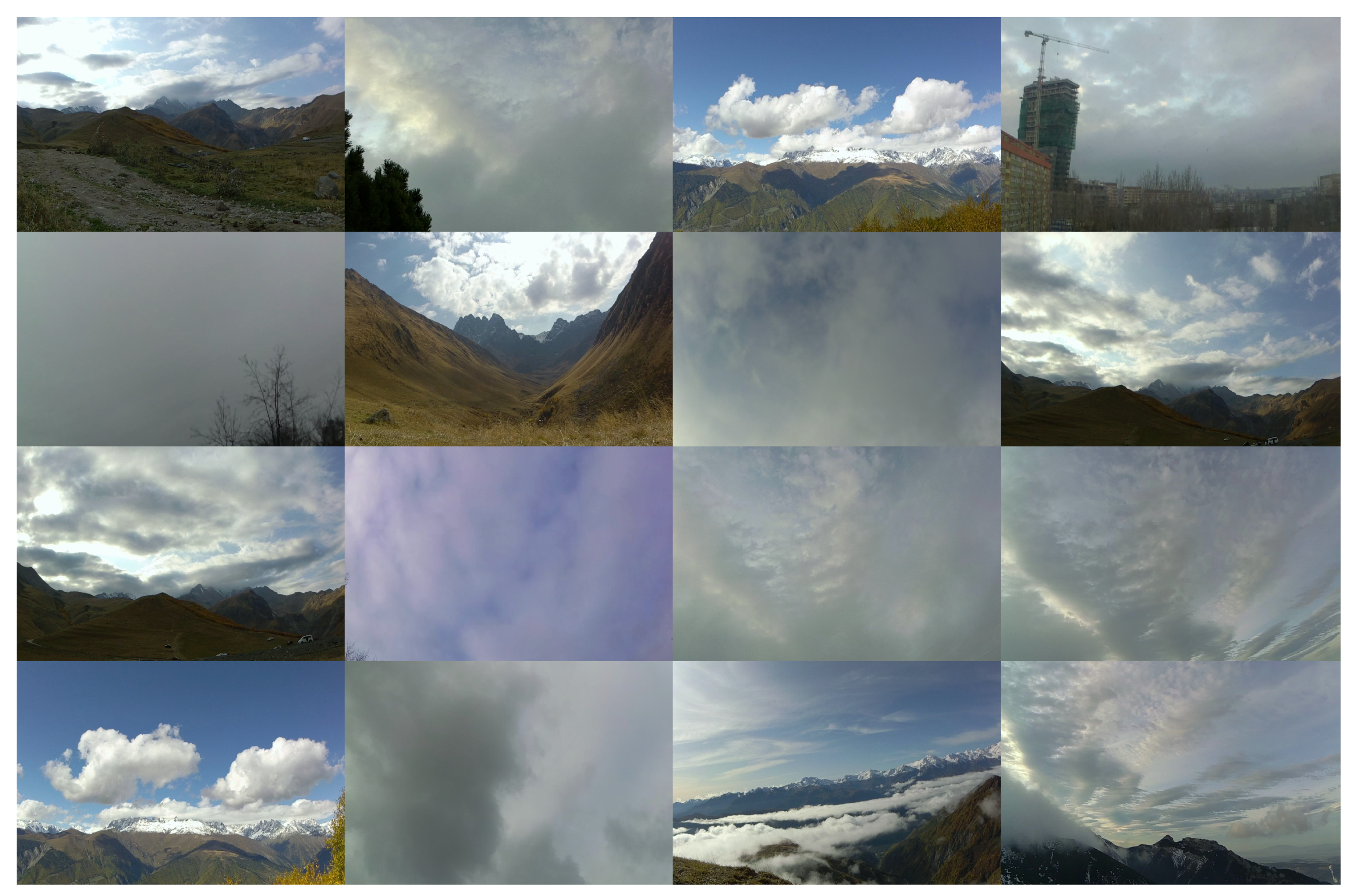
There are many types of clouds and their appearance additionally depends on the solar azimuth and elevation angle. The height of the observation site (camera placement) also affects the visibility of the clouds; for example, in mountainous regions, it is possible to observe the clouds from above. This article uses a publicly available database developed by the authors (https://github.com/sanczopl/CloudDataset, accessed on 5 January 2021). The recordings were made with different cameras with different settings. Exemplary image frames for different sequences are shown in Figure 1.
The video sequences were recorded with 30 fps; the resolution was and , and the duration was 30 s (900 frames). This article assumed an analysis of the grayscale video sequences.
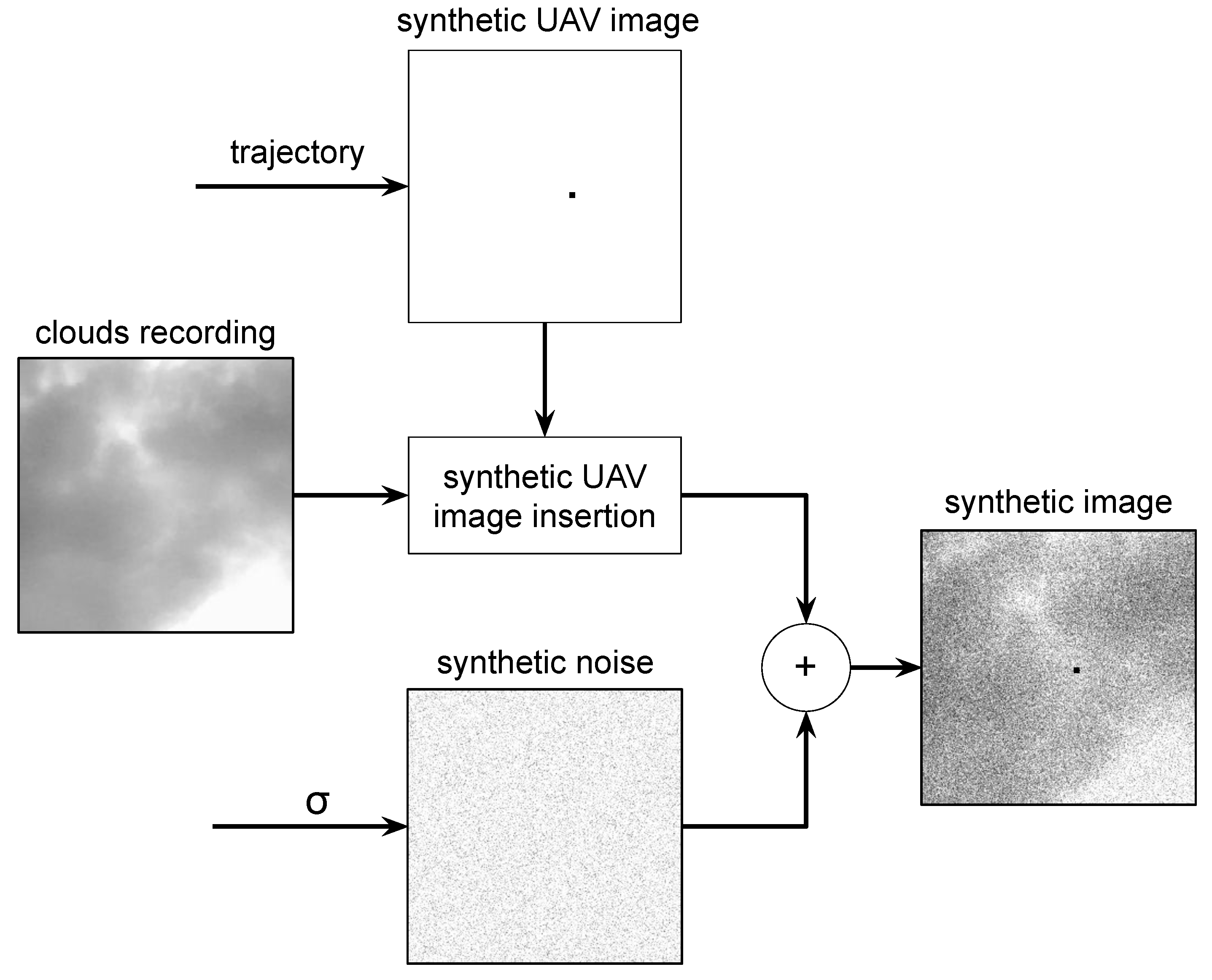
2.2. Augmentation Process
The use of real UAV sequences makes it difficult to analyze the algorithms because it is necessary to collect a very large number of video sequences for various conditions. This limits the ability to test algorithms. It is more effective to use sequences with combined UAV, background, and noise image. This makes it possible to control the trajectory of the UAV and the level of image noise. Additive Gaussian noise is controlled by the (standard deviation) parameter. The image-merging process is shown in Figure 2.
Background estimation algorithms may use the information of only one image frame in order to compute the background. Algorithms of this type are relatively simple or use a rich database of images. A more typical solution is the use of algorithms that use a certain sequence of a few or a dozen image frames for background estimation, which means that they can adapt to various conditions and are not limited by the database.
A certain disadvantage of using previous image frames is the creation of transient effects. In the case of algorithm studies, this can be controlled by placing the UAV within range not from the first frame. This ensures that the algorithm is initialized correctly. This article assumes that the UAV arrives from frame no. 300. Real tracking systems do not require this type of additional assumptions because they work continuously.
3. Method
The two main problems with the use of background estimation algorithms are selection of the right algorithm and selection of the parameters. Selection of the correct algorithm can be made by independent benchmarking, as done in the next section. Choosing the best set of parameters is a task for the optimization algorithm. In the case of this work, there are two cascade-connected algorithms: the background estimation algorithm and the threshold algorithm. In this case, optimization concerns all parameters of the algorithms. It is also possible to optimize the system via background estimation algorithm replacement with another and via related change in the number and significance of the parameters; however, this option was not used to compare the algorithms.
As the reference images (ground truth) are known, it is possible to use criteria for a comparison with the estimated images. A genetic algorithm was used as an optimization algorithm and a metric—fitness value—was proposed.
3.1. Background Estimation Algorithms
Background estimation algorithms allow for removing the background from the image through a subtraction operation. This allows us to reduce biases that affect further signal processing algorithms. In the case of thresholding, the chance of a false target detection for positive bias decreases and the chance of skipping target detection for negative bias is decreased. In TBD algorithms, the falsely accumulated signal value is reduced. Background estimation together with the operation of subtracting the estimated background from the current frame allows for background suppression. The tracked UAV is then easier to detect, although the image is disturbed by the noise related to acquisition. Depending on the background estimation algorithm and scene dynamics (moving clouds and lighting change), additional disturbances appear, the reduction of which is important for the tracking system. Limiting the number of false detections affects the computation complexity of multiple-target tracking algorithms.
The analysis of the relationship between the tracking algorithm and the background estimation algorithm is computationally complex; therefore, this research focused on the correctness of single UAV detection and reduction of tracking algorithm artifacts at different levels of image sensor noise.
The considered background estimation algorithms are listed in Table 1. Additionally, the programming itself without background estimation was used as the reference algorithm. Algorithm parameters and their range of parameters are specific for a given method (Table 1); therefore, it is practically impossible in the process of selecting the optimal algorithm to coordinate these results between the algorithms.
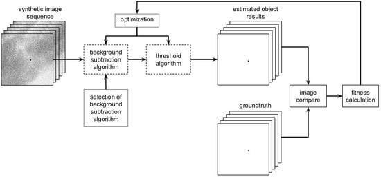
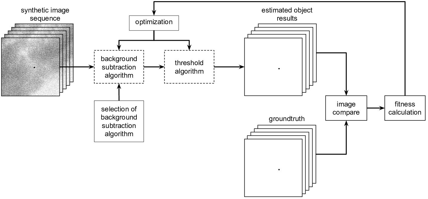
3.2. Background Estimation Pipeline
Dedicated optimization software was developed for pipeline implementation, which is shown in Figure 3. OpenCV 4.4.0 was used for image processing. The background estimation algorithms are also from the library https://docs.opencv.org/4.4.0/d7/df6/classcv_1_1BackgroundSubtractor.html, accessed on 5 January 2021. Algorithms requiring a GPGPU (General Purpose GPU) with CUDA (Compute Unified Device Architecture) support were not considered. It is important to use an SSD (Solid-State Drive) to store video sequences as they are read frequently. The software was written in C++ so that other algorithms can be added. Evaluation of the algorithm’s effectiveness also depends on the noise immunity in the image. For this purpose, the Monte Carlo approach was used, thanks to which it was possible to process data independently. This analysis uses distributed computing with 14 computers (8 cores per processor). JSON files were used to store the configuration of individual algorithms, including the range of parameter variability and the variable type (integer, float, double, and bool). The configuration for controlling the genetic algorithm was also saved in this format.
The full pipeline was used in the selection phase of the background estimation algorithm and its parameters as well as threshold value. In the normal operation phase, the selected algorithm was applied and the parameters of the background estimation algorithm as well as threshold were fixed. This means that the block “selection of background subtraction algorithm” is fixed and is not controlled by the optimization algorithm. The input images were 8-bit coded (grayscale), and the image after thresholding was a binary image.
3.3. Metrics Used for the Evaluation of Algorithms
Since background estimation allows for subtraction from video sequences, ideally their difference is only the UAV image. Thus, the Ground Truth (GT) sequence is a synthetically generated sequence with UAV images. The arithmetic difference of images in the sense of absolute values or logical difference can be used to test the algorithms. The arithmetic difference allows us to take into account the level of background estimation, for example, the degree of shadow estimation, while the binary variant is well suited for detection analysis. For a binary image representation, the value “1” corresponds to the position of the UAV and “0” represents the background for the specified pixel. By processing all pixels of the image, the values of TP (True Positive), TN (True Negative), FP (False Positive), and FN (False Negative) can be determined, which are the basic determinants of the work quality of the entire system including background estimation and thresholding. The values TP, TN, FP, and FN can be considered separate criteria for evaluation of the algorithm’s work quality. For the optimization process, however, it is necessary to determine one value of the objective function. For this reason, heuristics using the metric “fitness” have been proposed. The four individual metrics are determined by the following formulas:
All of them take values in the range . Finally, a fitness is determined from them, which takes values in the range :
3.4. Optimization Algorithm
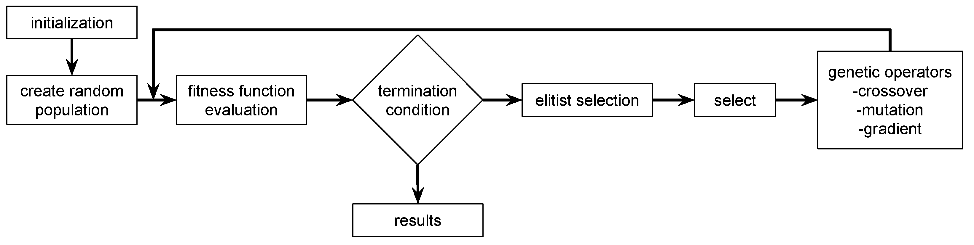
The individual algorithms were optimized independently of each other. Optimization was based on selection of the parameters of the background estimators and the threshold values. For optimization, a hybrid algorithm using genetic operators and gradient optimization were used [41,42]. Genetic algorithms are easy to implement, and because they do not use a gradient, they allow us to search for a global minimum. The block diagram of the algorithm is shown in Figure 4. Optimization is constrained as it affects known coefficient ranges (Table 1).
A pseudorandom number generator was used to initialize values for a particular background estimation algorithm and threshold value. This enabled the determination of binary strings describing the starting 30 individuals of the initial population and computing a first set of fitness values.
The elitist selection block is responsible for selecting the best and worst individuals. If the best individual is weaker than the best in the previous population, the weakest individual in the current population is replaced with the best in the previous population. The best current individual remains the same. If the best individual in the current population is better than the best individual in the previous population, it becomes the best current one.
The select block is used for fitness proportionate selection, also known as roulette wheel selection. The genetic algorithm uses two operators: crossover and mutation to change parameters [43,44]. There are many variants of crossover, in the case of the current implementation of the genetic algorithm, it is a k-point crossover. For the mutation operator, the value change was used as in evolutionary programming [41] because the range of values for a given algorithm is known.
There are several conditions for terminating the optimization process: achieving identical binary images compared on the output ( and ), and the maximum number of iterations is 20,000.
One of the problems with the optimization process is the lack of balance between the number of pixels in the image for the UAV and the number of background pixels. Without correction, a local minimum appears that is very difficult to remove. The introduction of corrections allows for balancing the error values related to the background and the UAV image. The values of FP and TP are corrected using the following formulas:
where is the UAV size in pixels.
4. Results
The Monte Carlo test allows us to obtain unbiased estimators [45,46] for a given algorithm, with the assumed noise value. The generated random video sequences constitute the input of the algorithm for which the parameters are optimized. Monte Carlo tests were performed for 8 algorithms, with 20 noise values each, and were executed 10 times (1600 cases).
Many computers are required for the computations, and Monte Carlo calculations can be paralleled. For the calculations, 14 computers with AMD Ryzen 7 processors and 16 threads for 8 processor cores were used. A single optimization case was computed by one thread and took approximately 2 h.
In the following subsections, exemplary results for the fitness value and the impact of the parameter values of the background estimation algorithms are presented. The most important are the results for Monte Carlo tests for different algorithms with different noise values, which allow us to assess their quality of work.
4.1. Exemplary Fitness Values
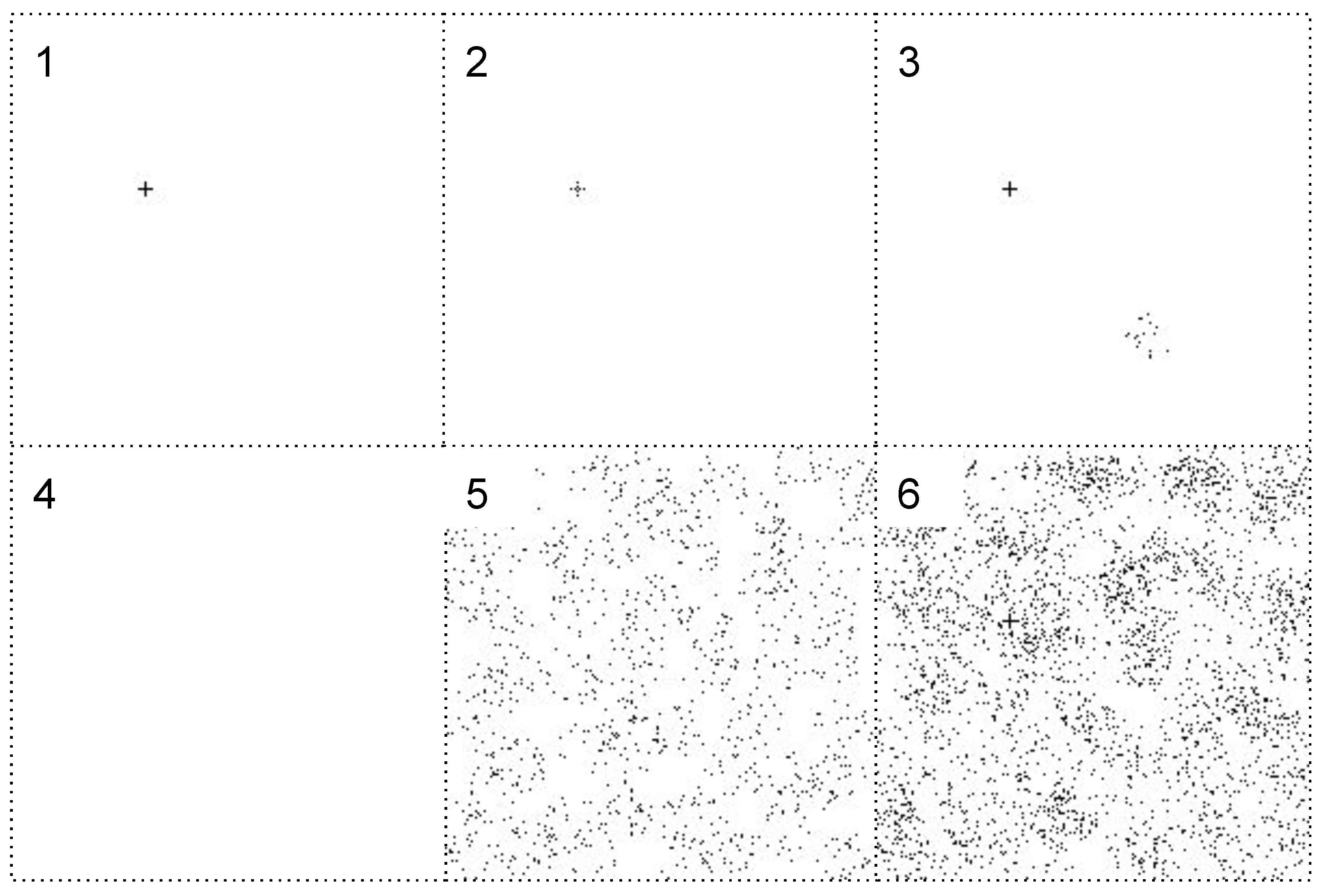
Several examples of synthetically generated images are shown in Figure 5, for which specific fitness values were obtained. In this case, the UAV is shaped similar to a plus sign for simplicity. There are also extreme cases, such as UAV and no noise, or no noise and no UAV.
4.2. Influence of Example Algorithm Parameters on the Detection Process
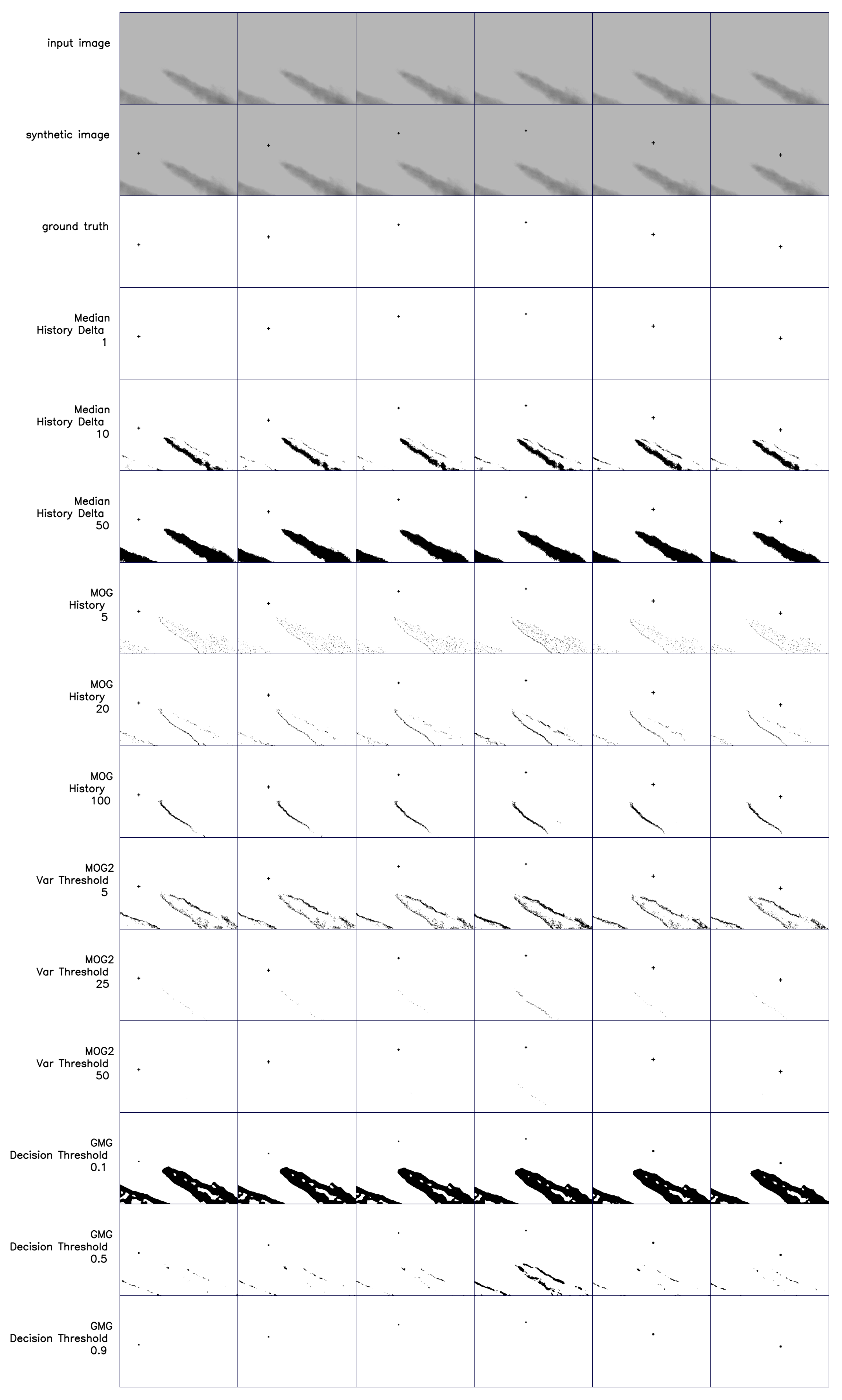
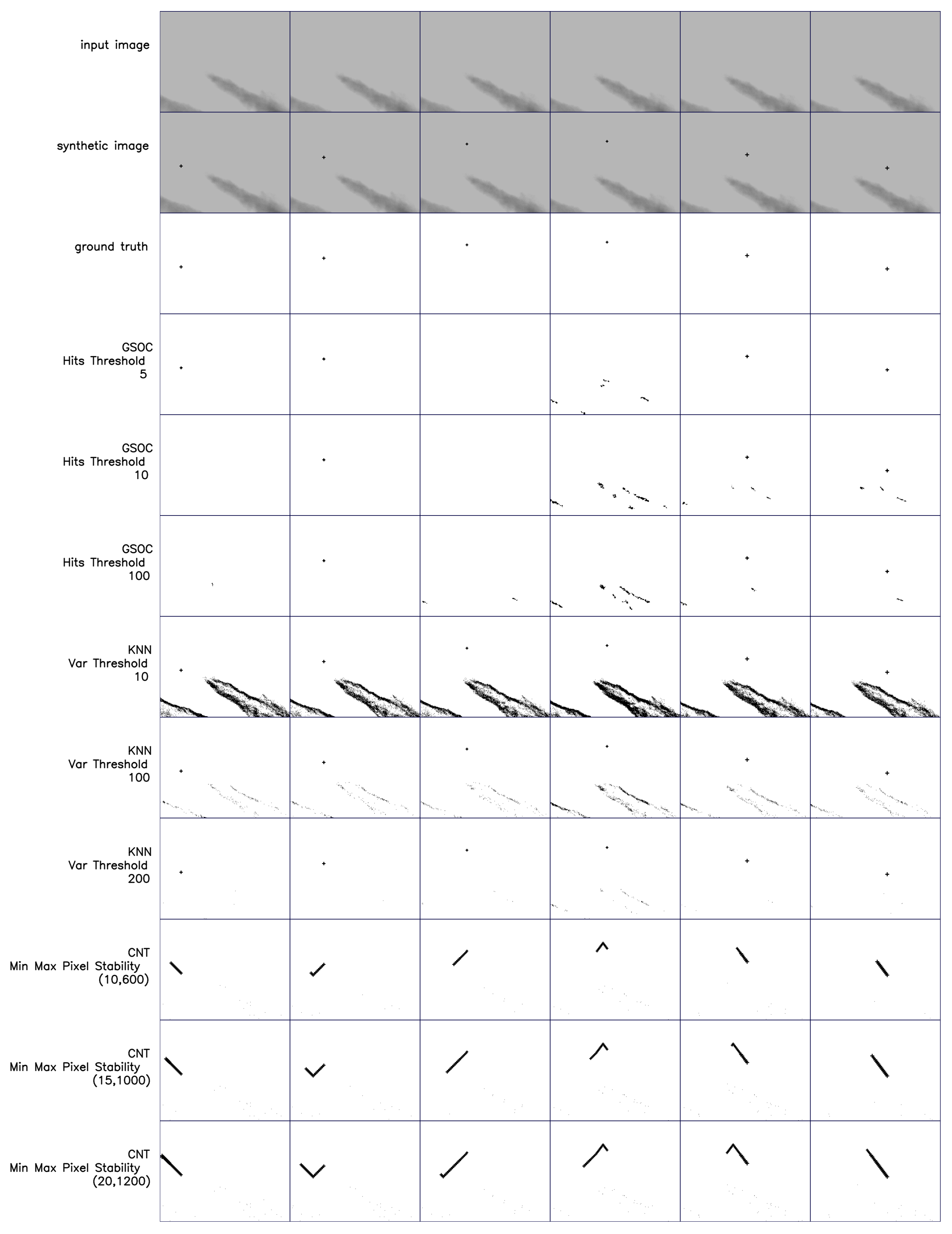
The problem of choosing the background estimation algorithm is related to the choice of parameters. Their selection affects the quality of the estimation, but it depends on the type of data, which makes manual selection by trial and error practically impossible. These parameters, although independent of each other according to their names, can create complicated relationships with each other, which complicates the search for the optimal configuration. Due to the large number of background estimation algorithms, selection of the optimal variant is a serious challenge. The influence of selected parameters on one video sequence is shown in Figure 6 and Figure 7.
4.3. Monte Carlo Analysis of Algorithms
The main computational goal in this article was to determine the fitness value for individual algorithms for different noise values.
In order to compare the results for the different algorithms, the random image sequences were the same. The number of repetitions (20) was experimentally selected due to a long processing time. In the case of bad converency of the genetic optimization processes or too little number of repetitions, the results from Figure 8 are very noisy. In the case of other applications of the method, it is necessary to test the degree of convergence each time to evaluate the algorithms.
Algorithms that better estimate the background and do not remove the UAV from the image have a fitness value closer to 4. Figure 8 shows the fitness averages for eight configurations, including no background estimation algorithm (NONE) as a reference.
Selection of the background estimation algorithm for a given noise level may introduce the problem of an excessive adjustment to the current noise level. To reduce this type of bias in the results, the fitness values with increased noise ( and ) are also shown for a given noise level. Thanks to this, it is possible to assess the sensitivity of the estimation algorithm and selected parameters to the increased noise level that did not occur during learning (optimization). Learning of the algorithm, through the selection of its parameters, is always limited by the training base used. This is particularly important when real (empirical) data are used, such as video sequences in this case. By adding noise in a certain range, the data can be augmented, which correlates to generalization in a learned system. This is a standard procedure to obtain an approximator rather than an interpolator that fits the data. The use of noise is also good for testing the resulting system. In the testing process, an increased noise level was used, where +10 and +20 noise were arbitrarily selected. If a given algorithm and its parameters are well matched, there should be no deterioration of the results for increased test noise by +10 and +20. Where there is a deterioration in the results, it means that another algorithm should be chosen as less sensitive.
4.4. Quantitative Results and Senstivity
One method of evaluating the algorithms is to determine the average value of the fit level, which is averaged. As the noise values ranged from 0 to 100, due to the sensitivity analysis, it was limited to the mean in the range 0 to 80. The mean values are presented in Table 2.
4.5. Computational Cost
The estimated computational cost was determined for a video sequence containing 1000 frames. The calculations were performed for 100 cases, and the mean value was determined. An image size of (grayscale) pixels was assumed. As modern processors perform frequency scaling (frequency change depending on load), scaling was turned off on purpose. Additionally, the video sequences were placed in the ramdisk so that downloading them from the SSD (Solid-State Drive) did not affect the result. This corresponds to the typical situation when consecutive video frames are delivered from the camera. The values given in the Table 3 are estimates because better results can be obtained by using different methods of code optimization.
A computer with a Intel i7–9750H @ 4 GHz processor was used for the estimation. The computations were allocated to one processor core.
5. Discussion
The most important computational result is the fitness curves for different types of background estimation algorithms (Figure 8). By analyzing their shape and values, the quality of individual algorithms can be compared. As the optimization process was time-limited, it is possible to obtain different results due to the slow optimization convergence. However, experiments with different but similar noise values show that the curves are mostly smooth, which means that convergence is acceptable. Only in some cases, there are larger jumps in fitness values that may require additional, longer empirical analysis.
5.1. Influence of Example Algorithm Parameters
The simple case of the UAV and two clouds shown in Figure 6 and Figure 7 shows that selection of the algorithms and parameter values for the algorithms should not be accidental. It is not possible to present all relations between several parameters for a given algorithm, so it was decided to show only a few examples for selected parameters.
In the case of the MEDIAN algorithm, too high a history delta value can lead to a lack of cloud elimination. For the MOG (MOG stands for Mixture of Gaussian) algorithm, the history parameter determines the balance between cloud edge detection and noise associated with cloud value changes. In the MOG2 (MOG stands for Mixture of Gaussian version 2) and KNN (K–Nearest Neighbor–based Background/Foreground Segmentation Algorithm) algorithms, a too low value of the Var threshold parameter leads to the detection of cloud edges and noise in the cloud area. The behavior is similar in the GMG (Godbehere-Matsukawa-Goldberg) algorithm for the decision threshold parameter. In the case of the GSOC algorithm and the hits threshold parameter, the number of detections can be highly variable depending on the image frame. The pair of pixel stability parameters can lead to the determination not so much of the detection but of the UAV trajectory.
5.2. Monte Carlo Analysis
Figure 8 shows the mean values obtained in the Monte Carlo experiments. The three algorithms CNT (CouNT), KNN and GMG give much worse results in relation to the others. Even with a low noise level, the quality of their background estimation is poor. They are even worse compared to just thresholding (NONE).
Other algorithms have a similar shape to the curve, but three parts of it are important: the fitness level for small noise values, the starting point of the curve descent, and the fitness level for large noise values. The MOG and GSOC algorithms have better properties for higher noise values than the others but at the cost of lower quality of work with low noise levels. The MEDIAN, MOG2, and NONE algorithms have very good properties for small noise values; however, as the noise value increases, they are worse than MOG and GSOC. The threshold algorithm NONE is inferior to MOG2 and may be rejected.
In the case of low noise, MOG2 is the best choice, although the MEDIAN algorithm is also interesting. The assessment of which one has better properties is carried out in the next subsection.
5.3. Sensitivity Analysis
Without the analysis of sensitivity to noise changes, the MEDIAN algorithm could be considered the best. Adding more noise to the video sequence than used during the training changes the characteristics of the algorithms. This is most evident for algorithms that are poor at low noise (CNT, KNN, GMG, and MOG). In the case of MEDIAN, the change is very large despite very good properties for low and high noise.
This experiment shows that, without empirical analysis of the sensitivity of algorithms, their evaluation or selection for a specific application can be very wrong. Using many different noise values for the algorithm testing process in one test can also be problematic due to averaging of the results.
5.4. Quantitative Results and Senstivity
Using this quantitative criterion, it can be seen (Table 2) that the apparently best algorithm is MEDIAN (column +0). When a more robust algorithm is required to increased noise that did not occur during the selection of parameters, MOG2 or GSOC is a better solution (columns +10 and +20).
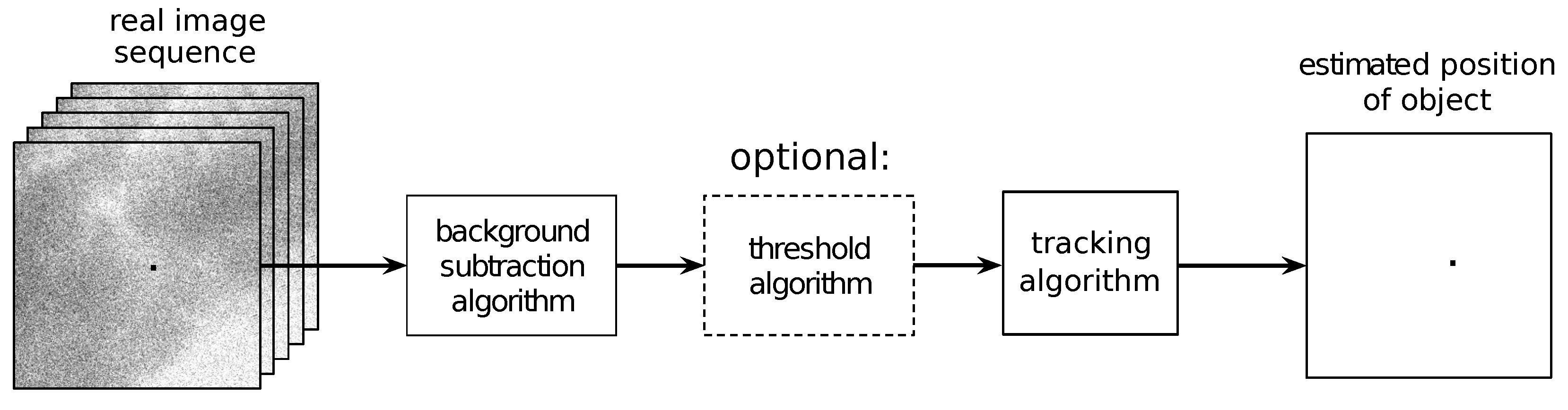
5.5. Thresholding and Tracking Approach
In this approach, we consider the selection of the background estimator for the tracking system, not the tracking system as a whole. Thresholding aims to define the criteria for selecting an algorithm and selecting coefficients. The selected algorithm along with the coefficients can then be used in the tracking system. With conventional tracking systems, the selected thresholding is still used and the data is passed to a tracking algorithm such as a Kalman filter (Figure 9). In the case of TBD systems, thresholding may be used, but it will reduce the tracking abilities. A much better solution is to omit thresholding so that the raw data (output of background subtraction algorithm) is processed by the TBD algorithm in accordance with the tracking-before-detection concept.
5.6. Computational Cost
As predicted, the simplest algorithm (NONE) is the fastest, in which the thresholding operation is performed without background estimation. The second fastest, but approximately 3 times slower, is the CNT algorithm. Another is the MOG2 algorithm, which is about 25 times slower than NONE.
The MOG2 and GSOC algorithms have been described as some of the most effective. This means that MOG2 is optimal both in terms of quality and computation time, as GSOC is very slow—about 10 times slower than MOG2. The MEDIAN algorithm has a computational cost similar to MOG2, and both can be treated as similar; however, MEDIAN has worse features due to the sensitivity to increased noise. For this reason, MOG2 seems to be the optimal solution. However, this assessment is burdened with an implementation error because, depending on the optimization of the source code and the compiler used, the results may differ.
A serious problem of most of the considered background estimation algorithms is the computational cost. In the case of a camera recording 25 fps images, the time to process one frame is 40 ms, and for a camera working at 100 fps, it is only 10 ms. The values extrapolated for a single 1 Mpix frame show that this time is mostly exceeded (Table 2). Background estimation algorithms are suitable for parallel processing, so implementation of a real-time system is possible, but effective code optimization is very important. An alternative is a hardware-based implementation, such as FPGAs (Field-Programmable Gate Array).
5.7. Real-Time Adaptation Possibility
There are at least three strategies for adapting algorithms (changing parameters) and selecting them for a real-time system.
The first strategy is an offline strategy. Video sequences are recorded and then subjected to optimization processes as presented in the article. This means that a suitable sample of the video sequence is needed. In the case of a background that is quite stable, which depends on the weather conditions, it is possible to obtain correct selection results quickly, so a proper image processing system for UAV detection can obtain a good quality configuration. In the case of a highly variable background, it depends on the degree of background change, and this depends on the region, climate, and season.
Due to the scale of calculations, data processing is possible in cloud computing. Typical resources for a nested device implementing a smart camera are too weak to perform such an operation with the current state of computing technology.
The second type of strategy is an attempt to adapt online algorithms (real-time adpatation), which is possible (similar to the classical adaptation algorithms used for example for adaptive filtering). The problem is the analysis of convergence of algorithms to background changes. It should be noted that, on a sunny day with rapidly moving clouds at low altitude, changes in lighting are rapid, sometimes less than one second. This strategy seems very attractive but creates a problem related to the stability of UAV detection.
A third possible strategy is a combination of both. The selection of the algorithm can be made once, and the range of parameter changes can be determined on the basis of previous video sequences. In this case, the parameter adaptation can be done in real time. It is also possible to narrow the range of parameters to the range determined by a certain index classifying the image. In this case, it is possible to develop a classifier that determines the type of image (for example, clear sky, cloudy sky, clouds at low altitude, etc.), which narrows the range of optimization parameters or even selects them directly. It is possible to implement, although it is a very complex task.
The presented adaptation strategies are not considered in this paper due to their complexity and scale of calculations.
5.8. Optimizing Background Estimation in Other Applications
The detection of small objects in the image is a problem not only related to UAV detection. An example is a reverse configuration, where the UAV image is analyzed for objects on the ground. Detection and tracking of vehicles, boats, and people is often carried out using thermal imaging systems, where the background can be very complex [47]. This could be used for human search-and-rescue or surveilance purposes. The publication [48] shows an example of swimmer detection. The problem of background estimation concerns not only vision systems but also radar imaging [49,50]. Application of the detection of small objects in medicine is also very important [51].
The proposed method is universal and can significantly improve the quality of other systems. Of course, the selection of algorithms and parameters may be different than in the work obtained in relation to UAVs.
6. Final Conclusions and Further Work
MOG turned out to be the best algorithm because it has very good properties for low noise values and for high noise values and is robust to increased noise value. Considering the results from Figure 8, one can consider a hybrid solution switching between two algorithms depending on noise. By using image noise level estimation, it is possible to use MOG2 for small noise values and the MOG algorithm for larger values. Taking into account the speed of execution of individual algorithms indicates that MOG2 is the most interesting to use.
The optimization method used in this article is an offline process. A high calculation cost of optimization is required for one-time selection of an algorithm and calculation of coefficients. An alternative is implementation of the adaptation process, which selects factors depending on the current conditions. In this case, the approach proposed in this article can be used to select an algorithm for which the coefficients are calculated online.
The proposed optimization solution can be applied to other types of tracked objects, not only UAVs. This work did not consider tracking algorithms that additionally implement a data filtration process. Including them in the overall optimization process as well as in the initial processing of images will be the subject of further work.
Author Contributions
Conceptualization, G.M. and P.M.; methodology, G.M and P.M.; software, G.M.; validation, G.M.; formal analysis, P.M.; investigation, G.M.; resources, P.M.; data curation, G.M.; writing—original draft preparation, G.M and P.M.; visualization, G.M.; supervision, P.M.; project administration, P.M. All authors have read and agreed to the published version of the manuscript.
Funding
This research received no external funding.
Institutional Review Board Statement
Not applicable.
Informed Consent Statement
Not applicable.
Data Availability Statement
The article uses a publicly available database developed by the authors: https://github.com/sanczopl/CloudDataset (accessed on 5 January 2021). The recordings were made with different cameras with different settings.
Acknowledgments
This work was supported by equipment purchased under the project: UE EFRR ZPORR project No.Z/2.32/I/1.3.1/267/05 “Szczecin University of Technology—Research and Education Center of Modern Multimedia Technologies” (Poland).
Conflicts of Interest
The authors declare no conflict of interest.
References
- Blackman, S.S.; Popoli, R. Design and Analysis of Modern Tracking Systems; Artech House: Norwood, MA, USA, 1999. [Google Scholar]
- Farlik, J.; Kratky, M.; Casar, J.; Stary, V. Multispectral Detection of Commercial Unmanned Aerial Vehicles. Sensors 2019, 19, 1517. [Google Scholar] [CrossRef] [PubMed] [Green Version]
- Ezuma, M.; Erden, F.; Anjinappa, C.K.; Ozdemir, O.; Guvenc, I. Micro-UAV Detection and Classification from RF Fingerprints Using Machine Learning Techniques. In Proceedings of the IEEE Aerospace Conference, Big Sky, MT, USA, 2–9 March 2019; pp. 1–13. [Google Scholar]
- Schüpbach, C.; Patry, C.; Maasdorp, F.; Böniger, U.; Wellig, P. Micro-UAV detection using DAB-based passive radar. In Proceedings of the IEEE Radar Conference (RadarConf), Seattle, WA, USA, 8–12 May 2017; pp. 1037–1040. [Google Scholar]
- Sedunov, A.; Salloum, H.; Sutin, A.; Sedunov, N.; Tsyuryupa, S. UAV Passive Acoustic Detection. In Proceedings of the IEEE International Symposium on Technologies for Homeland Security (HST), Woburn, MA, USA, 23–24 October 2018; pp. 1–6. [Google Scholar]
- Bell, K.L.; Corwin, T.L.; Stone, L.D. Bayesian Multiple Target Tracking, 2nd ed.; Artech House: Norwood, MA, USA, 2013. [Google Scholar]
- Archana, M.; Geetha, M.K. Object detection and tracking based on trajectory in broadcast tennis video. Procedia Comput. Sci. 2015, 58, 225–232. [Google Scholar] [CrossRef] [Green Version]
- Boubekeur, M.B.; Luo, S.; Labidi, H. A background subtraction algorithm for indoor monitoring surveillance systems. In Proceedings of the IEEE International Conference on Computational Intelligence and Virtual Environments for Measurement Systems and Applications (CIVEMSA), Shenzhen, China, 12–14 June 2015; pp. 1–5. [Google Scholar]
- Cheng, C.Y.; Hsieh, C.L. Background estimation and correction for high-precision localization microscopy. ACS Photon. 2017, 4, 1730–1739. [Google Scholar] [CrossRef]
- Zhou, X.; Zou, Y.; Wang, Y. Accurate small object detection via density map aided saliency estimation. In Proceedings of the IEEE International Conference on Image Processing (ICIP), Beijing, China, 17–20 September 2017; pp. 425–429. [Google Scholar]
- Ogorzalek, J.; Doyle, D.; Black, J. Autonomous Small Unmanned Aerial Systems Computer Vision Tracking. In Proceedings of the AIAA Aviation 2019 Forum, Dallas, TX, USA, 17–21 June 2019; p. 3050. [Google Scholar]
- Chen, P.Y.; Hsieh, J.W.; Gochoo, M.; Wang, C.Y.; Liao, H.Y.M. Smaller Object Detection for Real-Time Embedded Traffic Flow Estimation Using Fish-Eye Cameras. In Proceedings of the IEEE International Conference on Image Processing (ICIP), Taipei, Taiwan, 22–25 September 2019; pp. 2956–2960. [Google Scholar]
- Zeevi, S. BackgroundSubtractorCNT. 2017. Available online: https://sagi-z.github.io/BackgroundSubtractorCNT/ (accessed on 5 January 2021).
- Godbehere, A.B.; Matsukawa, A.; Goldberg, K. Visual tracking of human visitors under variable-lighting conditions for a responsive audio art installation. In Proceedings of the American Control Conference (ACC), Montreal, QC, Canada, 27–29 June 2012; pp. 4305–4312. [Google Scholar]
- KaewTraKulPong, P.; Bowden, R. An improved adaptive background mixture model for real-time tracking with shadow detection. In Video-Based Surveillance Systems; Springer: Boston, MA, 2002; pp. 135–144. [Google Scholar]
- Zivkovic, Z.; Van Der Heijden, F. Efficient adaptive density estimation per image pixel for the task of background subtraction. Pattern Recognit. Lett. 2006, 27, 773–780. [Google Scholar] [CrossRef]
- Zivkovic, Z. Improved adaptive Gaussian mixture model for background subtraction. In Proceedings of the 17th International Conference on Pattern Recognition, ICPR 2004, Cambridge, UK, 26 August 2004; Volume 2, pp. 28–31. [Google Scholar]
- Chen, M.; Wei, X.; Yang, Q.; Li, Q.; Wang, G.; Yang, M.H. Spatiotemporal GMM for background subtraction with superpixel hierarchy. IEEE Trans. Pattern Anal. Mach. Intell. 2017, 40, 1518–1525. [Google Scholar] [CrossRef]
- Song, S.b.; Kim, J.H. SFMOG: Super Fast MOG Based Background Subtraction Algorithm. J. IKEEE 2019, 23, 1415–1422. [Google Scholar]
- Cioppa, A.; Van Droogenbroeck, M.; Braham, M. Real-Time Semantic Background Subtraction. arXiv 2020, arXiv:2002.04993. [Google Scholar]
- Yang, B.; Jia, Z.; Yang, J.; Kasabov, N.K. Video Snow Removal Based on Self-adaptation Snow Detection and Patch-based Gaussian Mixture Model. IEEE Access 2020, 8, 160188–160201. [Google Scholar] [CrossRef]
- Pei, S.; Li, L.; Ye, L.; Dong, Y. A Tensor Foreground-Background Separation Algorithm Based on Dynamic Dictionary Update and Active Contour Detection. IEEE Access 2020, 8, 88259–88272. [Google Scholar] [CrossRef]
- Shahbaz, A.; Jo, K.H. Improved Change Detector using Dual-Camera Sensors for Intelligent Surveillance Systems. IEEE Sens. J. 2020, 1–8. [Google Scholar] [CrossRef]
- Sobral, A. BGSLibrary: An OpenCV C++ Background Subtraction Library. In Proceedings of the IX Workshop de Visão Computacional (WVC’2013), Rio de Janeiro, Brazil, 3–5 June 2013. [Google Scholar]
- Sakkos, D.; Liu, H.; Han, J.; Shao, L. End-to-end video background subtraction with 3d convolutional neural networks. Multimed. Tools Appl. 2018, 77, 23023–23041. [Google Scholar] [CrossRef]
- Zeng, D.; Zhu, M. Background subtraction using multiscale fully convolutional network. IEEE Access 2018, 6, 16010–16021. [Google Scholar] [CrossRef]
- Liu, Y.; Yang, F.; Hu, P. Small-Object Detection in UAV-Captured Images via Multi-Branch Parallel Feature Pyramid Networks. IEEE Access 2020, 8, 145740–145750. [Google Scholar] [CrossRef]
- Fu, Z.; Chen, Y.; Yong, H.; Jiang, R.; Zhang, L.; Hua, X.S. Foreground gating and background refining network for surveillance object detection. IEEE Trans. Image Process. 2019, 28, 6077–6090. [Google Scholar] [CrossRef]
- Seidaliyeva, U.; Akhmetov, D.; Ilipbayeva, L.; Matson, E. Real-Time and Accurate Drone Detection in a Video with a Static Background. Sensors 2020, 20, 3856. [Google Scholar] [CrossRef]
- Magoulianitis, V.; Ataloglou, D.; Dimou, A.; Zarpalas, D.; Daras, P. Does Deep Super-Resolution Enhance UAV Detection? In Proceedings of the 16th IEEE International Conference on Advanced Video and Signal Based Surveillance (AVSS), Taipei, Taiwan, 18–21 September 2019; pp. 1–6. [Google Scholar] [CrossRef]
- Koksal, A.; Ince, K.; Alatan, A.A. Effect of Annotation Errors on Drone Detection with YOLOv3. In Proceedings of the IEEE/CVF Conference on Computer Vision and Pattern Recognition Workshops (CVPRW), Seattle, WA, USA, 14–19 June 2020; IEEE Computer Society: Los Alamitos, CA, USA, 2020; pp. 4439–4447. [Google Scholar] [CrossRef]
- Wang, Y.; Jodoin, P.M.; Porikli, F.; Konrad, J.; Benezeth, Y.; Ishwar, P. CDnet 2014: An expanded change detection benchmark dataset. In Proceedings of the IEEE Conference on Computer Vision and Pattern Recognition Workshops, Columbus, OH, USA, 23–28 June 2014; pp. 387–394. [Google Scholar]
- Sobral, A.; Vacavant, A. A comprehensive review of background subtraction algorithms evaluated with synthetic and real videos. Comput. Vis. Image Underst. 2014, 122, 4–21. [Google Scholar] [CrossRef]
- Choudhury, S.K.; Sa, P.K.; Bakshi, S.; Majhi, B. An evaluation of background subtraction for object detection vis-a-vis mitigating challenging scenarios. IEEE Access 2016, 4, 6133–6150. [Google Scholar] [CrossRef]
- Kalsotra, R.; Arora, S. A comprehensive survey of video datasets for background subtraction. IEEE Access 2019, 7, 59143–59171. [Google Scholar] [CrossRef]
- Garcia-Garcia, B.; Bouwmans, T.; Silva, A.J.R. Background subtraction in real applications: Challenges, current models and future directions. Comput. Sci. Rev. 2020, 35, 100204. [Google Scholar] [CrossRef]
- Bianco, S.; Ciocca, G.; Schettini, R. Combination of video change detection algorithms by genetic programming. IEEE Trans. Evol. Comput. 2017, 21, 914–928. [Google Scholar] [CrossRef]
- Alonso, M.; Brunete, A.; Hernando, M.; Gambao, E. Background-Subtraction Algorithm Optimization for Home Camera-Based Night-Vision Fall Detectors. IEEE Access 2019, 7, 152399–152411. [Google Scholar] [CrossRef]
- Solanki, D.; Gurjar, M.K. Improvement Productivity in Balancing Assembly Line by Using Pso Algorithm; IJSRET: Pune, India, 2019; Volume 5, pp. 1261–1264. [Google Scholar]
- Kucukkoc, I.; Karaoglan, A.D.; Yaman, R. Using response surface design to determine the optimal parameters of genetic algorithm and a case study. Int. J. Prod. Res. 2013, 51, 5039–5054. [Google Scholar] [CrossRef] [Green Version]
- Michalewicz, Z. Genetic Algorithms + Data Structures = Evolution Programs; Springer Science & Business Media: Berlin/Heidelberg, Germany, 2013. [Google Scholar]
- Eiben, A.E.; Smith, J.E. Introduction to Evolutionary Computing; Springer: Berlin/Heidelberg, Germany, 2015. [Google Scholar]
- Koza, J.R.; Koza, J.R. Genetic Programming: On the Programming of Computers by Means of Natural Selection; MIT Press: Cambridge, MA, USA, 1992; Volume 1. [Google Scholar]
- Haupt, R.L.; Ellen Haupt, S. Practical Genetic Algorithms; Wiley-Interscience: Hoboken, NJ, USA, 2004. [Google Scholar]
- Metropolis, N.; Ulam, S. The Monte Carlo Method. J. Am. Stat. Assoc. 1949, 44, 335–341. [Google Scholar] [CrossRef]
- Kroese, D.P.; Brereton, T.; Taimre, T.; Botev, Z.I. Why the Monte Carlo method is so important today. Wiley Interdiscip. Rev. Comput. Stat. 2014, 6, 386–392. [Google Scholar] [CrossRef]
- Zhang, H.; Zhang, L.; Yuan, D.; Chen, H. Infrared small target detection based on local intensity and gradient properties. Infrared Phys. Technol. 2018, 89, 88–96. [Google Scholar] [CrossRef]
- Lu, Y.; Dong, L.; Zhang, T.; Xu, W. A Robust Detection Algorithm for Infrared Maritime Small and Dim Targets. Sensors 2020, 20, 1237. [Google Scholar] [CrossRef] [PubMed] [Green Version]
- El-Darymli, K.; McGuire, P.; Power, D.; Moloney, C. Target detection in Synthetic Aperture Radar imagery: A State-of-the-Art Survey. J. Appl. Remote. Sens. 2013, 7, 071598. [Google Scholar] [CrossRef] [Green Version]
- Liu, G.; Zhang, X.; Meng, J. A Small Ship Target Detection Method Based on Polarimetric SAR. Remote Sens. 2019, 11, 2938. [Google Scholar] [CrossRef] [Green Version]
- Wei, M.S.; Xing, F.; You, Z. A real–time detection and positioning method for small and weak targets using a 1D morphology–based approach in 2D images. Light. Sci. Appl. 2018, 7, 18006. [Google Scholar] [CrossRef]
Figure 1.
Exemplary video frames of clouds from database.

Figure 2.
Augmentation process.

Figure 3.
Background estimation pipeline and quality assessment.

Figure 4.
Optimization algorithm.

Figure 5.
Exemplary fitness values for synthetic images (1: UAV (Unmanned Aerial Vehicle) ground truth ; 2: UAV and small noise ; 3: UAV with local small noise cloud ; 4: UAV out of the range ; 5: noise only, UAV out of the range ; and 6: UAV and significant noise ).
Figure 5.
Exemplary fitness values for synthetic images (1: UAV (Unmanned Aerial Vehicle) ground truth ; 2: UAV and small noise ; 3: UAV with local small noise cloud ; 4: UAV out of the range ; 5: noise only, UAV out of the range ; and 6: UAV and significant noise ).

Figure 6.
Influence of example algorithm parameters on the detection process (part 1) (GMG (Godbehere-Matsukawa-Goldberg), MOG (Mixture of Gaussian), MOG2 (Mixture of Gaussian version 2)).
Figure 6.
Influence of example algorithm parameters on the detection process (part 1) (GMG (Godbehere-Matsukawa-Goldberg), MOG (Mixture of Gaussian), MOG2 (Mixture of Gaussian version 2)).

Figure 7.
Influence of example algorithm parameters on the detection process (part 2) (CNT (CouNT), GSOC (Google Summer of Code 2017), KNN (K–Nearest Neighbor–based Background/Foreground Segmentation Algorithm)).
Figure 7.
Influence of example algorithm parameters on the detection process (part 2) (CNT (CouNT), GSOC (Google Summer of Code 2017), KNN (K–Nearest Neighbor–based Background/Foreground Segmentation Algorithm)).

Figure 8.
Monte Carlo analysis: best fitness of individuals (value noise 100 corresponds to std. dev. = 1 for Gaussian noise).
Figure 8.
Monte Carlo analysis: best fitness of individuals (value noise 100 corresponds to std. dev. = 1 for Gaussian noise).

Figure 9.
Tracking pipeline with background estimation.


Table 1.
Background estimation algorithms applied in the optimization process.
| Algorithm | Parameters | Ranges | Description |
|---|---|---|---|
| CNT | min pixel stability | 10–20 | The BackgroundSubtractorCNT |
| [13] | max pixel stability | 600–1200 | project based on counting. |
| is parallel | True/False | (CNT stands for CouNT) | |
| use history | True/False | ||
| GMG | initialization frames | 1–200 | This algorithm combines |
| [14] | decision threshold | 0.01–1.0 | statistical background image |
| estimation and per-pixel | |||
| Bayesian segmentation (GMG: Godbehere-Matsukawa-Goldberg). | |||
| GSOC | camera compensation | True/False | It was implemented during GSOC |
| numbers of sample | 2–30 | and was not originated | |
| replace rate | 0.01–1.0 | from any paper. | |
| propagation rate | 0.01–1.0 | ||
| hits threshold | 1–255 | ||
| MOG | history | 1–200 | It is a Gaussian Mixture–based |
| [15] | N mixtures | 1–20 | Background/Foreground |
| background ratio | 0.01–1.0 | Segmentation Algorithm | |
| noise sigma | 0.01–1.0 | (MOG stands for Mixture of Gaussian) | |
| KNN | learning rate | 0.01–1.0 | K-nearest neighbor-based |
| [16] | history | 1–200 | Background/Foreground |
| var threshold | 1–255 | Segmentation Algorithm | |
| detect shadow | True/False | ||
| MOG2 | learning rate | 0.01–1 | Improved adaptive |
| [16,17] | history | 1–200 | Gaussian Mixture-based |
| var threshold | 1–255 | Background/Foreground | |
| detect shadow | True/False | Segmentation Algorithm (MOG stands for Mixture of Gaussian version 2) | |
| Median | history | 1–200 | Custom implementation |
| history delta | 1–30 | of median filter applied | |
| decision threshold | 1–255 | to sequence of images | |
| None | Empty block |
Table 2.
Mean values for the noise 0–80 range. The three best results are marked, and the highest value is underlined.
Table 2.
Mean values for the noise 0–80 range. The three best results are marked, and the highest value is underlined.
| Algorithm | +0 | +10 | +20 |
|---|---|---|---|
| CNT | 3.1143 | 3.0158 | 2.8118 |
| MEDIAN | 3.8941 | 3.8235 | 3.6294 |
| KNN | 2.9286 | 2.8052 | 2.6706 |
| MOG | 3.6249 | 3.5737 | 3.5685 |
| GMG | 3.1238 | 2.9468 | 2.9216 |
| MOG2 | 3.8294 | 3.8241 | 3.8235 |
| GSOC | 3.8235 | 3.8117 | 3.8023 |
| NONE | 3.6470 | 3.6389 | 3.6376 |
Table 3.
Mean values for computational time. The three best results are marked, and the highest value is underlined. Calculated for default parameter values.
Table 3.
Mean values for computational time. The three best results are marked, and the highest value is underlined. Calculated for default parameter values.
| Algorithm | Size for 1000 Frames (ms) | Size Single Frame Cost (ms) | 1Mpix Sensor Extrapolated Single Frame Cost (ms) |
|---|---|---|---|
| CNT | 1414 | 1.414 | 15.7 |
| MEDIAN | 7432 | 7.432 | 82.6 |
| KNN | 10210 | 10.210 | 113.4 |
| MOG | 6554 | 6.554 | 72.8 |
| GMG | 14162 | 14.162 | 157.4 |
| MOG2 | 5920 | 5.920 | 65.8 |
| GSOC | 75120 | 75.120 | 834.7 |
| NONE | 216 | 0.216 | 2.4 |
Publisher’s Note: MDPI stays neutral with regard to jurisdictional claims in published maps and institutional affiliations. |
© 2021 by the authors. Licensee MDPI, Basel, Switzerland. This article is an open access article distributed under the terms and conditions of the Creative Commons Attribution (CC BY) license (http://creativecommons.org/licenses/by/4.0/).
Share and Cite
MDPI and ACS Style
Matczak, G.; Mazurek, P. Comparative Monte Carlo Analysis of Background Estimation Algorithms for Unmanned Aerial Vehicle Detection. Remote Sens. 2021, 13, 870. https://doi.org/10.3390/rs13050870
AMA Style
Matczak G, Mazurek P. Comparative Monte Carlo Analysis of Background Estimation Algorithms for Unmanned Aerial Vehicle Detection. Remote Sensing. 2021; 13(5):870. https://doi.org/10.3390/rs13050870
Chicago/Turabian StyleMatczak, Grzegorz, and Przemyslaw Mazurek. 2021. "Comparative Monte Carlo Analysis of Background Estimation Algorithms for Unmanned Aerial Vehicle Detection" Remote Sensing 13, no. 5: 870. https://doi.org/10.3390/rs13050870
Note that from the first issue of 2016, this journal uses article numbers instead of page numbers. See further details here.