Article

Assessing Stream Thermal Heterogeneity and Cold-Water Patches from UAV-Based Imagery: A Matter of Classification Methods and Metrics

1
Aquatic Systems Biology Unit, TUM School of Life Sciences, Technical University of Munich, 85354 Freising, Germany
2
Department of Infrastructure Engineering, School of Engineering, University of Melbourne, Parkville, VIC 3010, Australia
*
Author to whom correspondence should be addressed.
Remote Sens. 2021, 13(7), 1379; https://doi.org/10.3390/rs13071379
Submission received: 12 February 2021 / Revised: 13 March 2021 / Accepted: 30 March 2021 / Published: 3 April 2021
(This article belongs to the Special Issue Application of Hyperspectral Data in Ecological Environment)

Abstract

:
Understanding stream thermal heterogeneity patterns is crucial to assess and manage river resilience in light of climate change. The dual acquisition of high-resolution thermal infrared (TIR) and red–green–blue-band (RGB) imagery from unmanned aerial vehicles (UAVs) allows for the identification and characterization of thermally differentiated patches (e.g., cold-water patches—CWPs). However, a lack of harmonized CWP classification metrics (patch size and temperature thresholds) makes comparisons across studies almost impossible. Based on an existing dual UAV imagery dataset (River Ovens, Australia), we present a semi-automatic supervised approach to classify key riverscape habitats and associated thermal properties at a pixel-scale accuracy, based on spectral properties. We selected five morphologically representative reaches to (i) illustrate and test our combined classification and thermal heterogeneity assessment method, (ii) assess the changes in CWP numbers and distribution with different metric definitions, and (iii) model how climatic predictions will affect thermal habitat suitability and connectivity of a cold-adapted fish species. Our method was successfully tested, showing mean thermal differences between shaded and sun-exposed fluvial mesohabitats of up to 0.62 °C. CWP metric definitions substantially changed the number and distance between identified CWPs, and they were strongly dependent on reach morphology. Warmer scenarios illustrated a decrease in suitable fish habitats, but reach-scale morphological complexity helped sustain such habitats. Overall, this study demonstrates the importance of method and metric definitions to enable spatio-temporal comparisons between stream thermal heterogeneity studies.

Graphical Abstract

1. Introduction

The role of stream temperature as a key aspect of rivers’ ecological functioning has received increasing attention in the last two decades [1,2,3]. Indeed, water temperature is a crucial player in all trophic levels and stages of biological organization in rivers. Water temperature governs the biochemical processes and conditioning of all freshwater life stages [4,5,6,7,8], highlighting the importance of understanding stream thermal heterogeneity. In addition, the predicted increase in water temperatures as a result of climate change [9] will likely grow the relevance of integrating the assessment and monitoring of stream temperature variability in future river management, particularly in identifying thermally resilient areas to changing climate [10,11,12,13,14].
Stream thermal heterogeneity is governed by a complex mosaic of interconnected habitats in rivers [15,16,17,18]. Though climatic, topographic, and hydrological controls drive stream temperatures at the air–water interface [1,2,3], multi-spatial scale factors such as in-stream morphology, groundwater inflow, and shading [3,19,20,21,22] shape its spatio-temporal variability.
The monitoring of stream thermal heterogeneity has been dramatically facilitated by the use of unmanned aerial vehicles (UAVs). In contrast to conventional single-point-data temperature measurements (e.g., temperature sensors and loggers), airborne surveys offer the advantage of providing optical and thermal image data over a wide area at a high spatial resolution [10,23]. UAVs have been extensively used to detect thermally differentiated patches in rivers, with a particular focus on biologically relevant cold-water patches (CWPs). Here, we refer to CWPs as discrete areas of cooler water in relation to the average water temperature in the mainstream channel [24]. CWPs are most relevant in summer as potential refugia during critically warm periods because cooler waters provide an oxygen-richer environment that may help the survival of mobile aquatic organisms such as fish [25,26,27].
Though there is a growing body of literature on the use of UAV surveys to assess stream thermal properties, the combined analysis of optical red–green–blue-band (RGB) and thermal infrared (TIR) imagery is still developing. Such a combination allows one to map thermally differentiated patches in rivers and to characterize their physical attributes, thus providing an integrated thermal–habitat assessment. However, most common UAV setups (consisting of one camera mount and a single camera with a basic global position system (GPS)) require two individual flights to obtain both RGB and TIR imagery. As a result, the acquired RGB and TIR imagery data present a spatial mismatch that requires complex and extensive post-processing to improve the overlapping match [24]. A specific challenge resulting from this mismatch is the need for manual geo-correction to accurately define the water edges in both TIR and RGB imagery to allow for the extraction of true water pixels for classification. Different approaches based on UAV remote sensing have been described in the literature for delineating the water edge or mapping lotic systems. These approaches include manual mapping [24], RGB imagery classification [28,29], using topographic data derived from RGB imagery [30,31] or from light detection and ranging [32,33,34,35,36], multispectral band ratio indices using near infrared (NIR) [37,38], UAV-based bathymetry derived from multispectral data [39,40], and object-oriented approaches [38]. Generally, the use of multispectral imagery poses challenges due to inherent spectral variability and shading [41,42,43]. While manual mapping approaches can result in the subjective characterization of features of interest, automatic approaches provide more standardized mapping methods; however, the latter also present challenges because they may require additional technologies for data acquisition and processing. Using additional sensing technologies to TIR and RGB imagery, for example, would most likely require numerous individual flights over the same area due to the limited camera mounts on a UAV, further post-processing efforts with difficulties in exact data overlay between flights, and differences in ground sampling size due to different sensor resolutions. Overall, to precisely delimit water vs. land cover poses challenges to current UAV-based imagery approaches for assessing water bodies [44], and, in turn, for deriving and analyzing stream thermal heterogeneity.
An additional challenge lies in the definitions of the thermal thresholds and physical habitat characterization of CWPs. These are not always harmonized, leading to a hampered comparability between study results. Though not always standardized, physical habitat characterization can be established using definitions of riverscape habitats (e.g., fluvial mesohabitats, riparian cover classes, and in-stream features). Most challenging is the establishment of thermal thresholds (temperature and area) to define CWPs consistently. This challenge lies in the inherent differences in river systems and the diversity of target freshwater species, which lead to case-specific definitions. From a technical perspective, many studies use the river thalweg’s temperatures (pixels alongside the thalweg line in a certain image or group of images) as a statistical average reference to identify CWPs [24,45,46,47,48,49] and likely as a way to avoid the challenging task to delimit and extract all TIR imagery true water pixels for the full thermal characterization of a river reach. Once the thermal reference is defined, CWPs are usually identified as areas between 0.5 and 3 degrees cooler than the mean reference, and their spatial dimensions can vary between 0.5 and 2.25 m2 of minimum area [12,22,24,45,48,50,51]. Such variation in CWP threshold definitions combined with the complexity of UAV-based imagery data acquisition, processing, and analysis have reduced the comparability of thermal heterogeneity and CWP studies.
The identification of CWPs is a key first step towards understanding the role of potential stream thermal refugia and a valuable tool to support river conservation and sustainable management [52,53]. Predictions of CWP locations and distribution, for example, can help identify species competitive advantages or disadvantages over native species under climate change (e.g., [54]). The development of tools to predict the distribution of potential thermal refugia in a riverscape will be critical to understanding the resilience of biological communities in stream systems, to inform long-term measures that maintain resilient thermal landscapes in future climate-change scenarios [10,47,55], and to aid the development of effective climate adaptation tools [56].
With the aim to optimize approaches to assess thermal heterogeneity via UAV-based imaging and to help facilitate the comparability between stream CWPs research, the specific objectives of this study were:
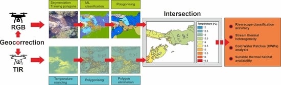
  • To provide a standardized approach for the combined analysis of UAV-obtained RGB and TIR imagery, including a supervised classification approach of fluvial mesohabitats based on spectral properties (RGB), and a thermal heterogeneity assessment linked to the thermal properties (TIR) of the classified habitats.
  • To quantify the changes in CWP numbers, distribution, and fluvial habitats with varying metric definitions, including thermal thresholds and patch size.
  • To assess the relevance of thermal heterogeneity changes in future climatic scenarios, as well as the consequence of thermal habitat availability, using rainbow trout (Oncorhynchus mykiss) as a model species.

2. Materials and Methods

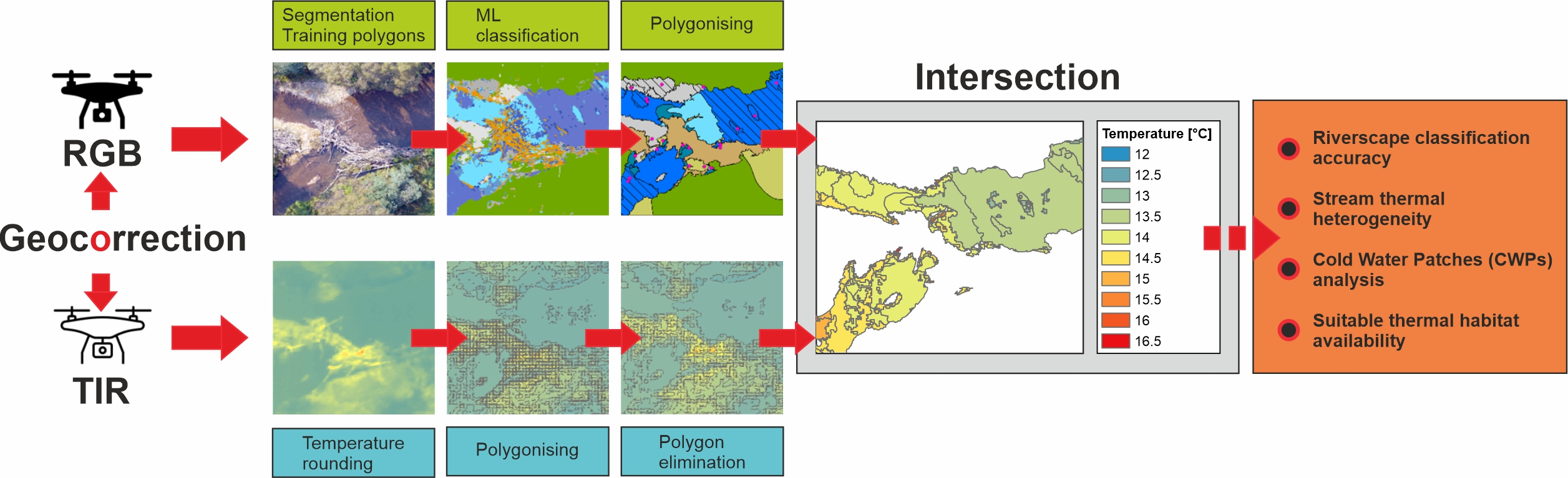
2.1. The Upper Ovens River

The Ovens River (Australia) is a 191-km-long north-east tributary of the Murray River with an annual discharge of 1776 GL.year−1. The catchment area covers 0.7% of the Murray Darling basin and contributes 6% of the basin water [57]. The river upstream of its junction with the Buffalo River near Myrtleford is designated as the Upper Ovens River with an approximate length of 70 km [58]. The Upper Ovens has been highlighted as one of the most unaltered catchments within the Murray–Darling Basin, considered to be a high value system that provides suitable habitat conditions for many fish species, including the endangered Murray cod (Maccullochella peelii peelii), and the introduced cold stenothermic European brown trout (Salmo trutta) and North American rainbow trout (Oncorhynchus mykiss) [59]. Due to the highly connected groundwater and surface water resources in the Upper Ovens [19] and the ambient climatic conditions, the river provided an ideal study location for assessing stream thermal heterogeneity and the potential to provide CWPs for cold-water-adapted fish species during heat periods in the summer month through pockets of upwelling cooler groundwater [24].

2.2. Dataset and Representative Reaches

The dataset used for this study was obtained from the extensive UAV-based imagery survey presented by Casas-Mulet et al. [24], carried out in a 50 km long (linear length) reach of the Upper River at the end of summer 2017 through a total of 49 flights. Each flight consisted of simultaneously obtained RGB and TIR imagery across 580–1600 m river lengths. Single RGB images were acquired by means of Phantom 4 Pro drone (DJI, Shenzhen China) equipped with an optical red–green–blue band camera (Zenmuse X5 RGB, DJI, Shenzhen, China). Single TIR images were acquired by simultaneously flying a second drone (Inspire 1 Pro, DJI, Shenzhen, China) that was equipped with a thermal infrared camera (Zenmuse XT, DJI, Shenzhen, China). TIR images were calibrated using the ResearchIR MAX TIR imagery analysis software (FLIR systems Inc., Wilsonville OR, USA). The imagery set corresponding to each flight was merged into a single orthomosaic using the photogrammetry software Pix4D (Pix4D S.A., Prilly, Switzerland). To rectify basic overlay, we used field ground control points (GCPs) geo-located utilizing a Leica© VivaGS14 real-time kinetics (RTK) differential global positioning system (dGPS). The GCPs had been placed along the survey area, subject to the limitations of the riverscape. They were manually deployed before the flights so they could be visible in both TIR- and RGB-obtained imagery. The imagery’s spatial resolution was 0.23 m per pixel in the TIR imagery and 0.035 m per pixel in the RGB imagery. For the TIR imagery, we used several in-situ water temperature point measurements and field-installed water loggers to correct and validate water temperature data, with a resulting correlation between logger value and corrected pixel data of R2 = 0.7. We considered that the UAV-based TIR caption of surface water temperatures was representative of the measurements across the whole water depth due to the following reasons: (i) although our surveys were carried out during the lowest flow period, water was still running through the system so hydraulic mixing was ensured, and (ii) several spot temperature measurements in selected deep pools illustrated almost identical temperatures across the water column [60], which supported our assumption of no thermal stratification. We accounted for spatio-temporal variations in water temperature by acquiring the data over five days of stable and similar weather conditions in the summer, correcting daily variations (morning vs. afternoon) with the use of logger data, and considering altitude and latitude variations by using relative-to-reach average temperatures. Full details on data acquisition and processing can be found in the work of Casas-Mulet et al. [24].
For the analysis in this study, we selected five orthomosaics as representative reaches of contrasting morphology, riparian vegetation, shading input, and degree of disturbance. Each of the selected reaches represented the overall variability that repeats along the Upper Ovens riverscape. The selected reaches or survey sections (S1, S2, S3, S4, and S5) were considered representative for the system, as per the criteria defined by Braun et al. [16]. S1 and S2 (1210 and 810 m, respectively) represented the most unaltered and natural river sections, with broadly open and dynamic braided channels surrounded by natural riparian vegetation. S3 and S4 were more constrained than the previous sites because they were limited by geological factors; however, they were both still meandering channels (of 930 and 1600 m, respectively) mostly surrounded by agricultural land use and a thin strip of overhanging riparian vegetation. S5, of 580 m reach length, represented the most altered river section that was heavily channelized and straightened (Figure 1).

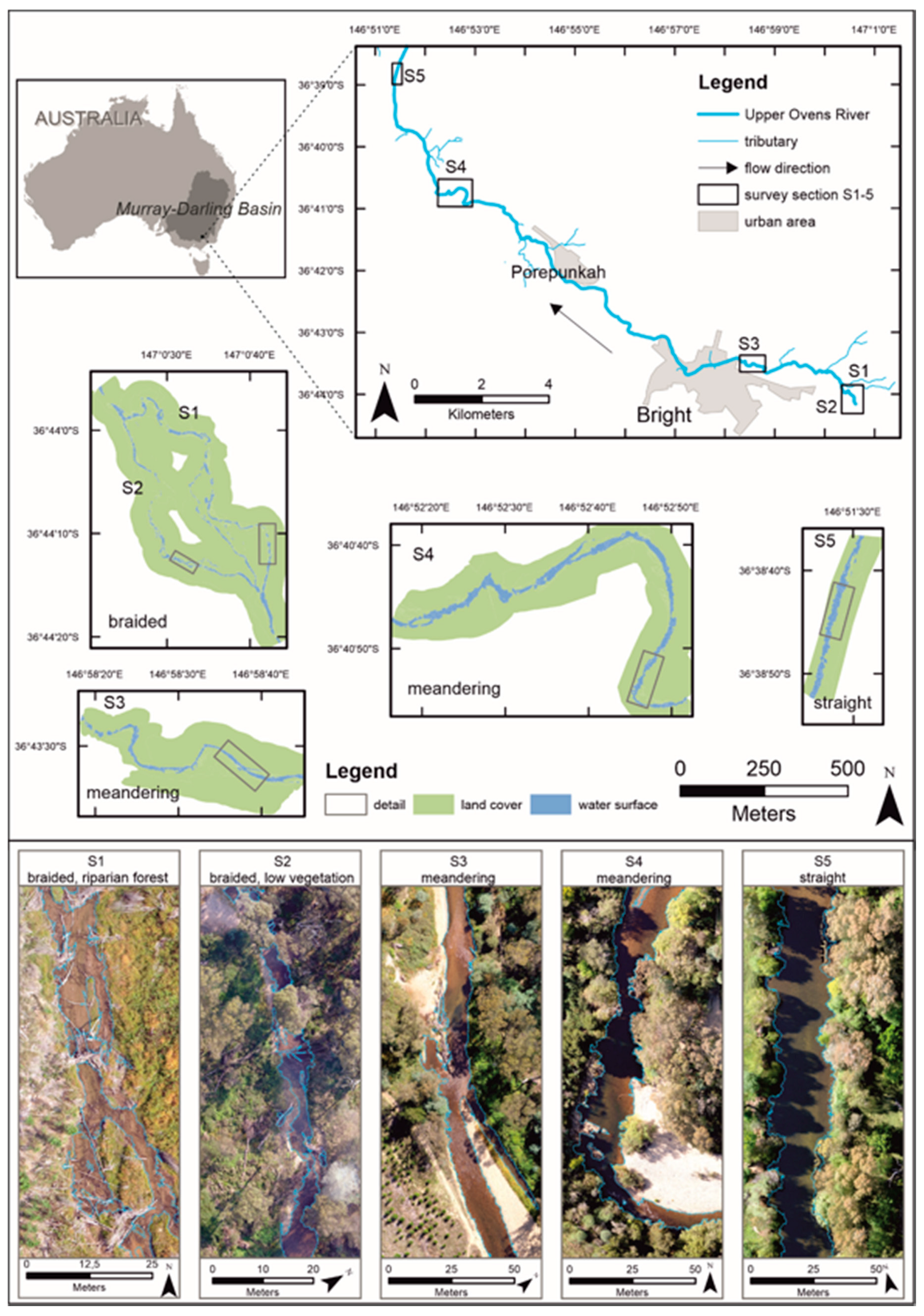
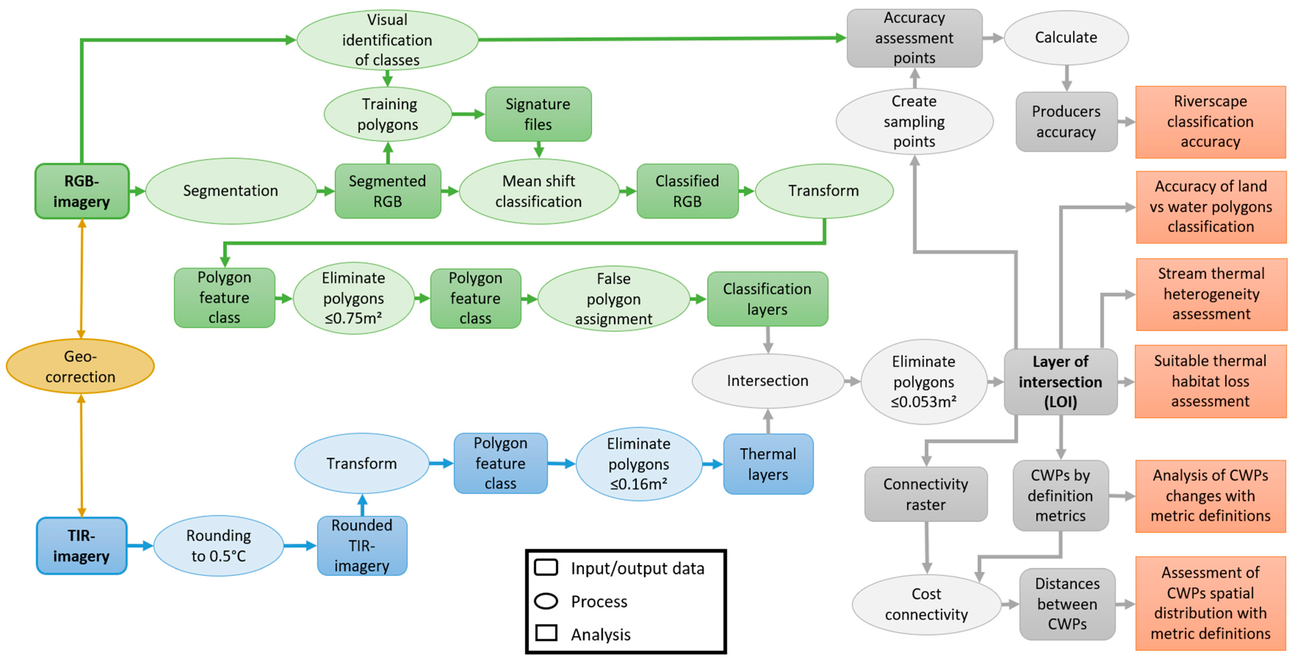
2.3. Data Processing

To enable the combined thermal–physical habitat analysis of the Upper Ovens, we classified and combined both RGB and TIR imagery data into an accurate spatially matching dataset created using the World Geodetic System (WGS) 1984 system as a reference (Universal Transverse Mercator Zone 55S), through the geoinformatics software ArcMap 10.6.1 (Esri, Redlands, CA, USA). Such classification and dataset matching were essential for later data analysis, and they followed the four main steps illustrated in Figure 2 and described below:

2.3.1. Geo-Correction and Overlay

We geo-corrected each RGB mosaic to perfectly match the corresponding TIR imagery set and enable accurate overlay for further analysis. In addition to GCPs, we used highly visible points of contrasting temperatures (e.g., end tip of in-stream heated up deadwood) in both TIR and RGB mosaics as reference points for third-order polynomial correction. We used between 16 and 32 geo-correction points for each pair of mosaics, resulting in an overlapping RMS (root mean square) error of 0.28 m. We did not quantify the planimetric accuracy before and after adding both GCPs and highly visible points of contrasting temperatures in both TIR and RGB mosaics. However, we observed that the initial mosaicking using GCPs only was not enough to enable an accurate matching overlay between TIR and RGB despite the RTK dGPS accuracy. The most likely reason was their non-uniform and sparse distribution along the riverscape, which reduced planimetric accuracy [61,62]. GCPs had been manually deployed over a geometrically irregular area (longer than wider, which is characteristic of all river reaches), and their locations were limited to spots of riparian vegetation openings. Therefore, additional reference points of contrasting temperatures were essential to ensure an accurate matching overlay rather than being used as checkpoints.

2.3.2. Supervised Classification of RGB Imagery

For each RGB mosaic, we classified the key components of the riverscape, including fluvial mesohabitats (MHs), in-stream fluvial geomorphic features (GFs), and riparian cover (RC). MHs were classified into “run”, “riffle”, “pool”, and “standing water” based on the appearance of the water surface structure to indicate flow velocity, depth visibility, and streambed substrate grain size [63,64,65]. We classified GFs into “gravel bar”, “bedrock”, and “dead wood”. RC was classified into “riparian forest”, “low vegetation”, and “plantation”. To account for the major effect that shading can have on stream temperatures [3], we distinguished between shaded and sun-exposed areas for each MH class and for the GFs classes “gravel bar” and “bedrock”.
For the supervised classification of each RGB mosaic into the MH, GF, and RC classes, we performed a "maximum likelihood classification" (options tool intern setting at zero reject fraction and equal priori probability) in ArcMap. We first segmented each RGB mosaic into pixel sets of similar spectral properties. We then drew training polygons over the identified MHs, GFs, and RCs to sample the mean spectral properties for each class. (Figure 2). Each training polygon sample was converted into a reference signature file (data with mean RGB band values of each class) for each RGB mosaic. We used, on average, 142 training polygons per mosaic or survey section and 32 training polygons for each class. The resulting classified RGB mosaic was transformed into a polygon feature class (further referred to as RGB-classified layer; see Figure 2). To minimize automatically false classified pixel-segments, which were a result of inherent spectral variability [43], we eliminated polygons of true area in the field of ≤0.75 m2 and manually assigned larger polygons that were wrongly classified to the correct class (Figure 2).

2.3.3. Conversion of TIR to Homogeneous Thermal Patches

Given that thermal emissivity fluctuations from a water surface structure can influence temperatures assignments [66,67,68], the temperature values of the TIR imagery were rounded to the closest half-degree Celsius [49]. Each TIR mosaic was then transformed into a polygon feature class composed of multiple polygons of the same temperature (further referred to as thermal layer). Single polygons smaller ≤3 pixels (true area in the field of ≤0.16 m²) were considered to be artefacts from the thermal camera sensor and were merged to the next larger polygon (Figure 2).

2.3.4. Combining Classification and Thermal Layers into a Single Dataset

To enable the analysis of riverscape features and their temperature, the thermal layers were intersected with the corresponding RGB-classified layer, resulting in a final intersected layer (further referred to as layer of intersection—LOI). Since the TIR imagery pixel resolution was lower than the RGB imagery resolution, the intersection resulted in some ≤1 pixel (true area in the field of ≤0.053 m²) polygons (or “silver polygons” [69]). These were eliminated by adding them to the next larger polygon of eachLOI (Figure 2). The mean stream temperature of all MHs (true water areas) in each thermal layer was used as a reference for further analysis, and it was calculated by summing up the area values multiplied by the temperature values of each water polygon, then divided by the total water polygon area. The resulting mean stream temperature from the polygonised thermal layer was compared to the value obtained by averaging the water temperature pixel values from the original TIR raster layer. The results were the same, suggesting that the raster to polygon conversion and rounding did not affect the temperature precision.

2.4. Data Analysis

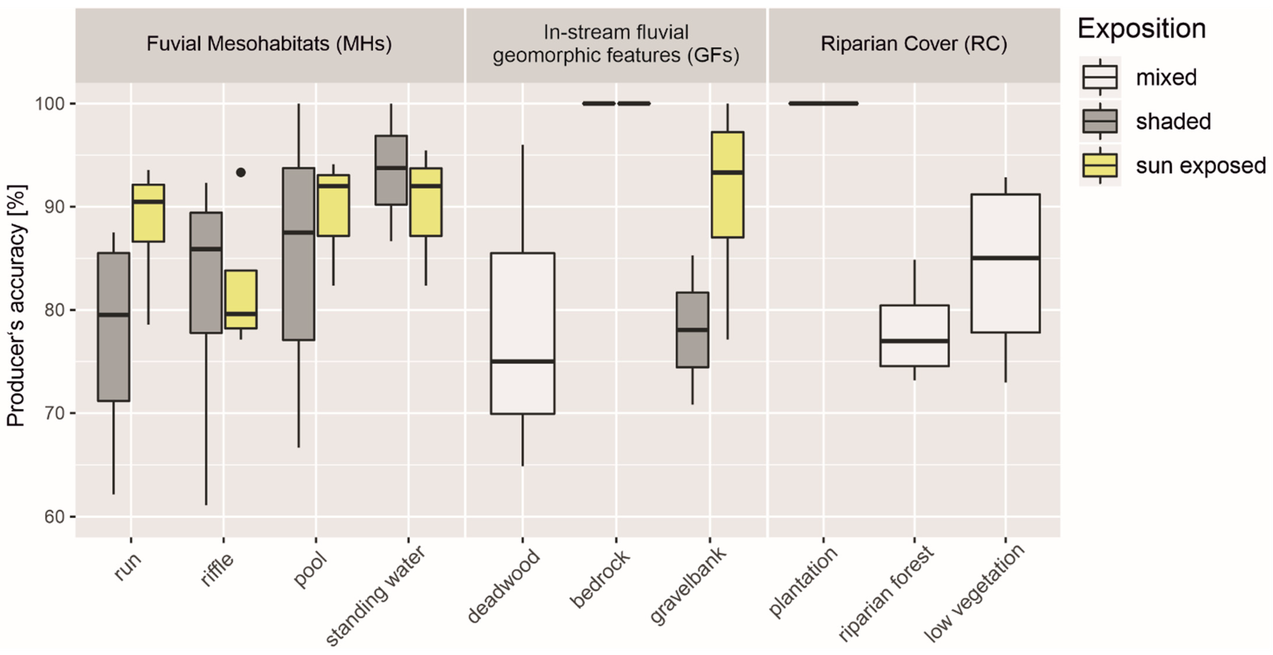
2.4.1. Riverscape Classification Accuracy

To assess the reliability of the supervised classification method, we compared the classification outcomes to ground truth through a visual interpretation of the RGB imagery. We quantitatively assessed 30 sampling points per class, distributed randomly in each of the 5 RGB-classified layers. We used the Producer’s accuracy indicator [70] to evaluate the agreement of the supervised classification method with the visual interpretation, calculated as the percentage of agreement between predicted (classified) and observed (visual interpretation) data.
As an additional test of data reliability, we assessed the accuracy of land vs. water polygon classification in each LOI by looking at the discrepancy between the temperature values and MH classification of small (single pixels) polygons at the water–land edges. Basically, the MH polygons of single pixels with high-temperature values at the water–land edge are realistically gravel banks (not water) and should be classified as land. However, because of the non-perfect match between TIR and RGB mosaics, we found that some of these high-temperature pixels were classified as water. To assess to what extent this mismatch could produce thermal inaccuracies, we compared our reference mean water temperature calculation (see Section 2.3.4) to the same calculation that excluded these high-temperature 1-pixel size outliers for each LOI.

2.4.2. Stream Thermal Heterogeneity Assessment

For each LOI, we assessed the frequency (number) and area of occurring temperatures, relative to each mean reference temperature, in all MHs. Data were tested for normality using the Shapiro–Wilk test. Since the frequency data of MHs were not normally distributed, we used Kruskal–Wallis to test global significant differences. As a post-hoc test for individual pairwise comparisons of temperature distributions between sunny and shaded MH classes, we used the pairwise Wilcoxon rank sum tests with Bonferroni correction to adjust p-values for multiple testing.

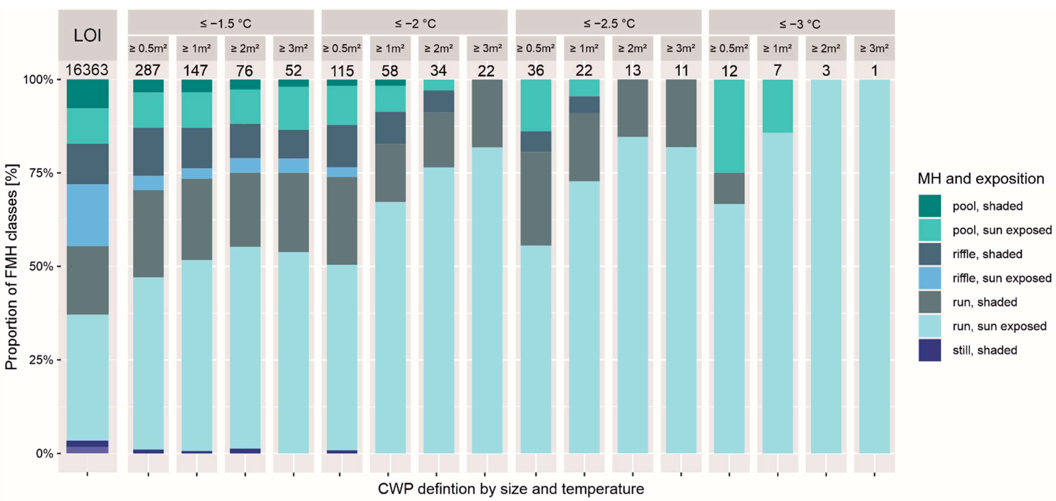
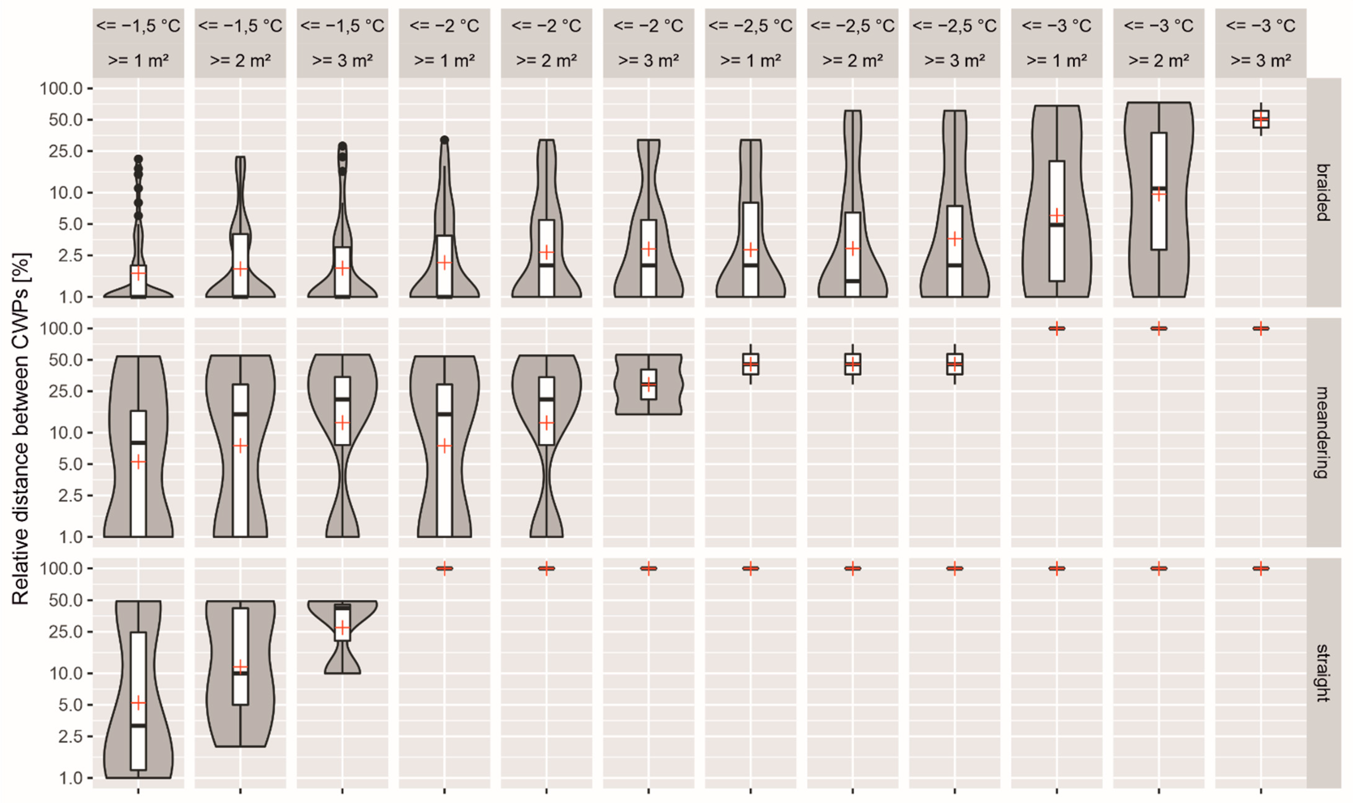
2.4.3. Analysis of CWP Changes with Metric Definitions

We assessed changes in CWP numbers and distribution with temperature and area threshold definitions. For temperature, we considered a range between 1.5 and 3 °C (0.5 °C steps) cooler than the average stream temperature. We considered an ecological relevant minimum area size of 0.5 m² [22] as a starting point and increased it in steps to a maximum of 3 m².
To assess the differences in CWP spatial distribution with changes in metric definitions, we computed the distances between the identified CWPs (start and end points being the start and end of the survey section) in each of three selected LOIs. These included one of each braided (S2), meandering (S4), and straight channel (S5). In order to ensure that distances were measured within the water body of the LOI, we used the attribute table tool in ArcMap to assign differentiated values between fluvial MHs (true water pixels), in-stream fluvial GFs, and RC classes and converted each LOI into a raster (connectivity raster; see Figure 2). Distances between CWPs were then analyzed with the “cost connectivity” tool in ArcMap using a total of 12 CWP metric definition combinations including areas of ≥1, ≥2, and ≥3 m² and relative temperature thresholds of ≤–1.5, ≤–2, ≤–2.5, and ≤−3 °C. To enable comparison between the selected LOIs or survey sections, the distances were calculated relative to each section’s total water body length. CWP clusters (distances of <3 m between CWPs) were considered as a single CWP. Distances between CWPs grouped by metric definition and survey section were tested for normal distribution using the Shapiro–Wilk test. Global significant differences in CWP distribution between metric CWP definitions within each survey section were tested using the Kruskal–Wallis test.

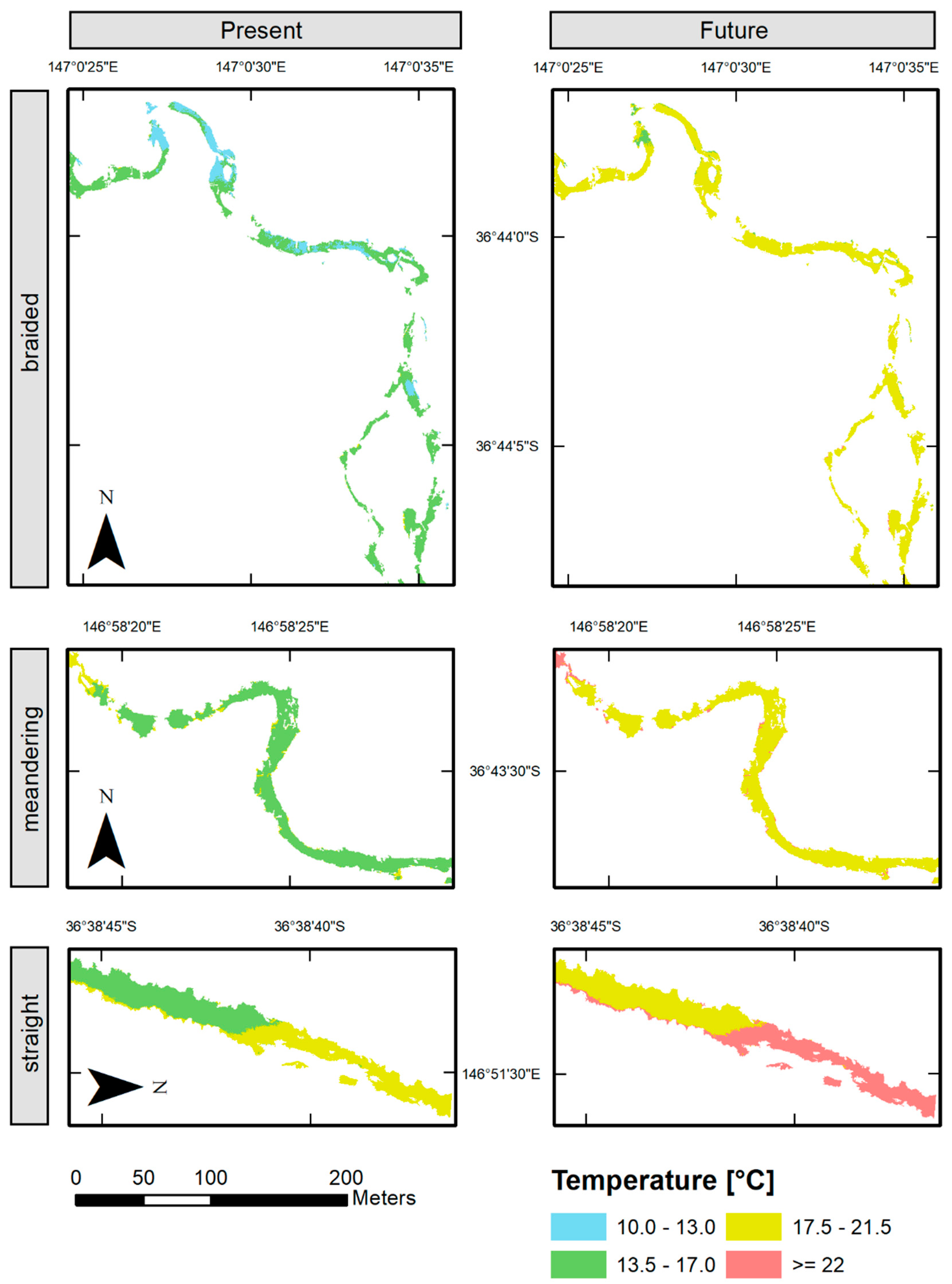
2.4.4. Suitable Thermal Habitat Loss Assessment

We assessed how stream temperatures could change with an increased water temperature of 4 °C based on potentially predicted future climatic scenarios [71,72]. In order to assess how these changes in stream thermal heterogeneity would impact suitable thermal habitats for fish, we used rainbow trout (Oncorhynchus mykiss) as a target species. Rainbow trout is a temperature-sensitive fish species that is very relevant for fisheries globally and is particularly abundant in the mainstream Upper Ovens [59]. We considered 17 °C as a preference water temperature threshold for rainbow trout [73,74] and 22 °C as a maximum limit [61]. We used the same representative S2, S3, and S5 sections to illustrate the assessment.
All statistical analyses were carried out using the open-source statistical software R [75]. Significance was accepted at p ≤ 0.05.

3. Results

3.1. Riverscape Classification Accuracy and Data Reliability

The supervised classification based on the spectral properties of water and their MHs, in-stream fluvial GFs, and RC resulted in a very high overall Producer’s accuracy for all classes (Figure 3). MH classification resulted in slightly better results (mean = 85.4% and std = 10.22%) compared to the GF and RC classification (GF mean = 86.17% and std = 10.89%; RC mean = 80.46% and std = 17.12%). In considering each class separately, an overall higher variability in Producer’s accuracy was found in shaded areas compared to sun-exposed MH (water) classes (Figure 3). Regarding land cover (GF and RC) classification, the lowest Producer’s accuracy was related to the classes “deadwood” and “gravel bar shaded,” whilst the highest Producer’s accuracy was found for “bedrock” and “plantation” classes (Figure 3). However, the "bedrock" class was only present in survey section S4. Our additional assessment of the effects of spatial mismatch that resulted in thermal inaccuracies suggested no significant differences between the reference mean water temperature calculation and the same calculation excluding high-temperature one-pixel size outliers for each LOI.

3.2. Stream Thermal Heterogeneity Linked to Fluvial Mesohabitats (MHs)

The frequency and areal distribution of temperatures for each fluvial MH class followed non-normal distributions (Shapiro–Wilk test: p ≤ 0.05) (Figure 4), showing an overall heterogeneity without a particular trend or pattern by MH class. Stream temperature frequencies presented significant differences between MHs (Kruskal–Wallis test: p < 0.001). As expected, pairwise comparisons confirmed that sun-exposed MHs were significantly warmer than shaded MHs (pairwise Wilcox rank sum test: p < 0.001), with a maximum difference in temperature of 0.62 °C. Most MHs presented warmer temperatures than the average stream temperature, illustrating that cooler water areas were not dominant. The presence of MHs with relative temperatures of ≤−1.5 °C (lower CWP thermal threshold) was highly variable in most classes (between 1.49% and 6.47% in frequency and between 0.48% and 2.94% in area size), except for standing sun-exposed water types, where temperatures were always above this threshold.

3.3. CWP Types, Frequency, and Distribution Changes with Metrics

Changing CWP definition metrics within the established thermal and areal thresholds influenced the amount of identified CWPs, as well as the relative proportion of the fluvial MHs they covered (Figure 5).
Following our expectation, the number of CWPs decreased as the thermal and areal thresholds were increased. Within a thermal threshold of ≤−1.5 °C, the number of CWPs decreased fivefold from ≥0.5 to ≥3 m²; however, the proportion of MH classes remained the same, following a similar pattern to the original river physical habitat composition (including both warm and cold patches). As thermal thresholds were increased, however, the proportion of MH classes changed from the original habitat composition and varied substantially between areal thresholds. The change in area share of MH composition was most sensitive with a shift from ≤−1.5 to ≤−2 °C. Such variable patterns, however, showed a consistent decrease in heterogeneity, with a loss of pool and riffle habitats, as area thresholds were increased (Figure 5).
The relative distribution of CWPs along each of the section types (braided, meandering, and straight) was not normally distributed (Shapiro–Wilk test p ≤ 0.05). Kruskal–Wallis tests revealed no global significant differences (p ≤ 0.14) in CWP distribution within each survey section. However, a visual assessment illustrated that changes in distribution were more sensitive to definition metrics in the straight channel (S5) than the braided channel (S2), which presented a smoother change in CWP distances based on metrics (Figure 6). Overall, the mean CWP distances increased with an increase of metric definition thresholds. However, the greatest increase in CWP distance occurred at different points of each of the representative reach—earlier (with lower temperature and areal thresholds) in the straight section and later (with higher temperature and areal thresholds) in the meandering and braided sections, suggesting that straight sections present faster changes and more complex sections present later shifts.

3.4. Present and Future Availability of Suitable Thermal Habitat

A predicted increase in water temperatures illustrated a clear shift in thermally suitable habitats for rainbow trout (Figure 7). Habitats below the optimum thermal limit (≤22 °C) were still available to a large extent in the braided and meandering sections (99.9% and 98.4%, respectively) but reduced in the straight section (90.1%). Preferred thermal habitats (≤17 °C) were least available in the braided section (16.6%) and completely disappeared in both the meandering and straight sections. The latter was only left with unsuitable thermal habitats (Figure 7), likely resulting in the local extinction of the considered fish species.

4. Discussion

This study presents a reliable semi-automatic approach to extract both physical habitat and stream thermal temperature information from UAV-based RGB and TIR imagery and to enable their combined analysis to assess changes in thermal heterogeneity and CWPs. Our thermal heterogeneity assessment did not show a particular trend or pattern by MH class but illustrated significant differences between shaded and non-shaded types. CWPs (using the lower relative temperature threshold of ≤−1.5 °C) were found in all except one MH; however, CWP numbers and the proportion of MHs they covered substantially changed with varying thermal and areal thresholds. The distribution assessment of CWPs revealed that this variability and metric sensitivity could be strongly linked to different types of reach morphology, with braided rivers being able to support bigger and cooler CWPs than straight channels. Such a reach morphology effect was also illustrated through the modelling of changes in a suitable thermal habitat with future predicted increases in water temperature. Channels with complex morphologies (braided and meandering) will provide more suitable thermal habitats for rainbow trout than simple straight channels in the future. These findings were based on the analysis of five characteristic reaches that reflected the full channel type variability along the riverscape. With each of them presenting a substantial reach length, they were considered representative of the ecohydrological processes occurring in the system. Overall, while acknowledging that any generalization needs to be made with care and that our dataset, although representative, was not exhaustive, we demonstrated that structurally homogenous river reaches are likely less resilient to increased temperatures than naturally braided ones in which CWPs are also sustained at increased ambient temperatures. Less complex or degraded channels can therefore bring potential local extinction consequences of cold-water-adapted species such as rainbow trout.

4.1. Riverscape Classification Accuracy and Data Reliability

Classification accuracy is crucial to assess the quality of thematic maps derived from remote sensing [70,76]. Our semi-automatic approach to riverscape classification was highly reliable to distinguish between riparian, in-stream, and water features, as well as to correctly classify them. A high Producer’s accuracy of classification and a low difference in mean temperature calculation by excluding unrealistic high temperatures at the land–water interface attested to the high reliability and spatial accuracy of the generated dataset. Excluding temperature outliers in the LOI for analysis to increase the reliability of the dataset was more conservative, for example, than using a buffer zone around banks and tree canopy [45]. The latter approach ensures the exclusion of unintended terrestrial temperatures, but it was not suitable for our dual TIR and RGB imagery analysis because it could have excluded valuable water pixel data at the water–land edge representing CWPs provided by lateral or hyporheic discharge (e.g., upwelling zones). Our approach to separate water vs. land pixels made it possible to calculate mean stream temperature using all true water pixels, and it provided a comprehensive representation of the overall channel temperature. Our approach differs from the most commonly used ones in the literature, in which the calculation is often limited to selected points along a river thalweg [24,45,46,47,48,49].
The fact that the data used in this study originated from two simultaneous but separated UAV flights (e.g., one for aerial RGB imagery and one for TIR imagery) posed a challenge for the exact georeferencing and overlapping of the two datasets. Still, our geo-correction approach achieved a precise matching between TIR and RGB with an RMS-error value similar to the smallest pixel size of the TIR imagery. Such a matching overlay enabled reliable water vs. land extraction and allowed for the analysis of stream water thermal heterogeneity. While our water vs. land extraction accuracy relied on RGB classification and was refined with the TIR–RGB discrepancy assessment (or LOI temperature outlier exclusion), such an approach was mostly possible due to the high contrast between land and water temperature in our dataset. In most cases, especially with low water–land contrast, the use of near infrared for water edge recognition would result in a higher accuracy of its delimitation. However, this system would still require an additional drone flight or camera mount, which was not available during our survey. Indeed, more advanced UAV setups that have two camera mounts or dual cameras combined with integrated, accurate spatial positioning technologies (e.g., RTK devices) may help the integration of multiple imagery data types in the future [77]. However, this recommendation can collide with regulations regarding UAV’s maximum take-off mass and flight scenarios in the vicinity of urban areas or uninvolved people (e.g., EU drone regulations [78]), so our approach for processing and combing RGB- and TIR-derived imagery by two separate (lighter) UAV flights does not lose any relevance.

4.2. Stream Thermal Heterogeneity Links to Fluvial Mesohabitats (MHs)

The combined supervised classification method for RGB imagery with the accurate TIR imagery match resulted in a suitable approach to extract temperature values for each identified fluvial MH, helping overcome geo-correction and overlay challenges. Our classification of shaded vs. sun-exposed MHs confirmed that shading can have a major effect on cooling water temperatures [11,22]. The overall classification of CWPs revealed that cold water areas are not bound to specific MH classes and confirmed the findings by Casas-Mulet et al. [24], suggesting that CWP controls span over multiple spatial scales beyond the meso-scale.

4.3. CWP’s Sensitivity to Metrics

Our analysis illustrated that the number, type, and distribution of CWPs change with varying definitions of temperature and areal thresholds. As expected, we found that as thermal and areal thresholds are increased, CWP numbers are reduced, their habitat heterogeneity decreases, and their distribution along the channel becomes sparser [10]. Changes in CWP numbers and distribution were found to strongly reflect different channel morphologies and landscape variables [12,24,50,79]. A single set of definition metrics provided significant differences in CWP distribution depending on the channel morphology; in straight channels, the number of CWPs decreased more rapidly with increased thermal and areal thresholds than in braided channels, reflecting the importance of complex morphology to sustain thermally differentiated areas. Regardless of the specific metric threshold, more complex river reaches can provide sufficient ranges of habitats that facilitate thermal heterogeneity and, in turn, promote CWPs; in contrast, straight channels require conservative thermal thresholds to enable the identification of differentiated thermal areas or CWPs due to their lower physical complexity [3,15,45,80,81]. The specific CWP definition metric thresholds used in this study fell within the range of definition metrics found in the literature [12,22,24,45,48,50,51,53], representing a broad variety of rivers in terms of size, morphology, and climatic context, as well as suggesting that our approach may enable potential comparisons. However, this study does not assume a direct transferability of results and does not attempt to provide a universal set of rules to identify and define CWPs. Rather, we consider our work the first development toward standard procedures and approaches for CWP assessments and comparisons.

4.4. Future Availability of Suitable Thermal Habitats for Fish

As expected, future climatic scenarios would reduce the spatial extent of thermally available habitats and reduce access to suitable refuge areas during climatic extremes. However, such reductions would be greater in less complex (i.e., structurally degraded) channels where thermally available habitats for fish would be substantially reduced as their distribution became sparser. Access to suitable habitats for rainbow trout was overall lower in simple straight channels than in complex braided reaches. Fish would hence need to swim further to reach suitable habitats in simple morphology reaches, suggesting a hindrance to fish population recruitment [82]. The structural deficits of river systems and their floodplains resulting from man-made channelization and river straightening are generally considered the main challenges in the conservation and restoration of riverine biodiversity (e.g., [13,83]). This is in line with our findings, highlighting the importance of in-stream river restoration measures to maintain thermally cooler water areas as potential thermal refugia in the future [84]. Our data, if computed at a large scale, might help to increase the number of remotely assessed water variables in the future. Future studies involving a combination of satellite and UAV-based TIR data can help predict large-scale thermal refugia occurrence, with a suite of potential applications to river ecologists and managers alike.

5. Conclusions

In conclusion, our approach to assessing combined UAV-based RGB–TIR imagery enabled an accurate integrated quantitative assessment of physical and thermal habitats. The identification of CWPs was sensitive to definition metrics but was also strongly linked to river morphological complexity, with complex channels able to support bigger and cooler CWPs in comparison to straight channels. Though this study does not attempt to provide a universal set of metrics to define CWPs, our findings help illustrate the importance of considering metric definitions and the fluvial geomorphology context to define CWP thresholds to (i) enable potential comparability between studies and (ii) develop standard procedures and approaches for CWP assessment in the future. The modelling of suitable thermal areas for cold-water fish estimated a decrease in suitable habitat for such species in the future, with warmer and less suitable waters compared to present conditions. The identified links with river morphological complexity and shading suggest that mitigation measures such as the restoration of channel complexity and establishment of bank vegetation can increase the resilience of fluvial systems to climatic change. The modelling approach presented here may generally be a powerful tool for predicting system resilience, prioritizing biological conservation, evaluating the effects of restoration measures, and supporting water resource management decisions.
In addition to its successful application in the Upper Ovens river, our approach can be easily transferred to other systems and climatic conditions, and results could be computed at a large scale using satellite data, for example. Our integrated approach should therefore be used to inform future climate adaptation measures and ensure the availability of suitable thermal habitats to sustain temperature-sensitive populations of freshwater biota.

Author Contributions

An equal first author contribution is considered for both authors J.K. and R.C.-M. Individual contributions are as follows: Conceptualization, R.C.-M., J.G., and J.P.; methodology, J.K. and R.C.-M.; formal analysis, J.K.; resources, J.G., J.P., and R.C.-M.; writing—original draft preparation, J.K. and R.C.-M.; writing—review and editing, R.C.-M., J.P., J.K., and J.G.; supervision, R.C.-M., J.P., and J.G.; project administration, J.P. and J.G.; funding acquisition, R.C.-M. All authors have read and agreed to the published version of the manuscript.

Funding

This research was funded by the Alexander von Humboldt Foundation, through a fellowship awarded to R.C.-M. and carried out at TUM.

Institutional Review Board Statement

Not applicable.

Informed Consent Statement

Not applicable.

Data Availability Statement

The data presented in this study are available on request from the corresponding author.

Acknowledgments

The authors would like to thank the North East Catchment Management Authority in Australia for the support during data collection, and the landowners for kindly providing access for the surveys. UAV-based surveys were carried out by XM3 Aerial Australia. We are grateful to the whole team of professionals, and students for their help during data acquisition in the field.

Conflicts of Interest

The authors declare no conflict of interest. The funders had no role in the design of the study; in the collection, analyses, or interpretation of data; in the writing of the manuscript, or in the decision to publish the results.

References

  1. Webb, B.W.; Hannah, D.M.; Moore, R.D.; Brown, L.E.; Nobilis, F. Recent advances in stream and river temperature research. Hydrol. Process. 2008, 22, 902–918. [Google Scholar] [CrossRef]
  2. Caissie, D. The thermal regime of rivers: A review. Freshw. Biol. 2006, 51, 1389–1406. [Google Scholar] [CrossRef]
  3. Poole, G.C.; Berman, C.H. An Ecological Perspective on In-Stream Temperature: Natural Heat Dynamics and Mechanisms of Human-Caused Thermal Degradation. Environ. Manag. 2001, 27, 787–802. [Google Scholar] [CrossRef] [PubMed]
  4. Canning, A.D.; Death, R.G. Ecosystem Health Indicators—Freshwater Environments. In Encyclopedia of Ecology, 2nd ed.; Fath, B., Ed.; Elsevier: Oxford, UK, 2019; pp. 46–60. [Google Scholar]
  5. Breau, C.; Cunjak, R.A.; Peake, S.J. Behaviour during elevated water temperatures: Can physiology explain movement of juvenile Atlantic salmon to cool water? J. Anim. Ecol. 2011, 80, 844–853. [Google Scholar] [CrossRef] [PubMed]
  6. Beitinger, T.L.; Bennett, W.A.; McCauley, R.W. Temperature Tolerances of North American Freshwater Fishes Exposed to Dynamic Changes in Temperature. Environ. Boil. Fishes 2000, 58, 237–275. [Google Scholar] [CrossRef]
  7. Warren, D.R.; Robinson, J.M.; Josephson, D.C.; Sheldon, D.R.; Kraft, C.E. Elevated summer temperatures delay spawning and reduce redd construction for resident brook trout (Salvelinus fontinalis). Glob. Chang. Biol. 2012, 18, 1804–1811. [Google Scholar] [CrossRef]
  8. Angilletta, M.J.; Niewiarowski, P.H.; Navas, C.A. The evolution of thermal physiology in ectotherms. J. Therm. Biol. 2002, 27, 249–268. [Google Scholar] [CrossRef]
  9. Van Vliet, M.T.H.; Ludwig, F.; Kabat, P. Global streamflow and thermal habitats of freshwater fishes under climate change. Clim. Chang. 2013, 121, 739–754. [Google Scholar] [CrossRef]
  10. Fullerton, A.H.; Torgersen, C.E.; Lawler, J.J.; Steel, E.A.; Ebersole, J.L.; Lee, S.Y. Longitudinal thermal heterogeneity in rivers and refugia for cold water species: Effects of scale and climate change. Aquat. Sci. 2018, 80, 1–15. [Google Scholar] [CrossRef]
  11. Garner, G.; Malcolm, I.A.; Sadler, J.P.; Hannah, D.M. The role of riparian vegetation density, channel orientation and water velocity in determining river temperature dynamics. J. Hydrol. 2017, 553, 471–485. [Google Scholar] [CrossRef]
  12. Wawrzyniak, V.; Piégay, H.; Allemand, P.; Vaudor, L.; Goma, R.; Grandjean, P. Effects of geomorphology and groundwater level on the spatio-temporal variability of riverine cold water patches assessed using thermal infrared (TIR) remote sensing. Remote Sens. Environ. 2016, 175, 337–348. [Google Scholar] [CrossRef]
  13. Geist, J.; Hawkins, S.J. Habitat recovery and restoration in aquatic ecosystems: Current progress and future challenges. Aquat. Conserv. Mar. Freshw. Ecosyst. 2016, 26, 942–962. [Google Scholar] [CrossRef]
  14. Ebersole, J.L.; Wigington, P.J.; Leibowitz, S.G.; Comeleo, R.L.; Van Sickle, J. Predicting the occurrence of cold-water patches at intermittent and ephemeral tributary confluences with warm rivers. Freshw. Sci. 2015, 34, 111–124. [Google Scholar] [CrossRef]
  15. Wohl, E. Connectivity in rivers. Prog. Phys. Geogr. Earth Environ. 2017, 41, 345–362. [Google Scholar] [CrossRef]
  16. Braun, A.; Auerswald, K.; Geist, J. Drivers and Spatio-Temporal Extent of Hyporheic Patch Variation: Implications for Sampling. PLoS ONE 2012, 7, e42046. [Google Scholar] [CrossRef] [Green Version]
  17. Thorp, J.H.; Thoms, M.C.; Delong, M.D. The riverine ecosystem synthesis: Biocomplexity in river networks across space and time. River Res. Appl. 2006, 22, 123–147. [Google Scholar] [CrossRef]
  18. Frissell, C.A.; Liss, W.J.; Warren, C.E.; Hurley, M.D. A hierarchical framework for stream habitat classification: Viewing streams in a watershed context. Environ. Manag. 1986, 10, 199–214. [Google Scholar] [CrossRef]
  19. Yu, M.C.L.; Cartwright, I.; Braden, J.L.; De Bree, S.T. Examining the spatial and temporal variation of groundwater inflows to a valley-to-floodplain river using 222Rn, geochemistry and river discharge: The Ovens River, southeast Australia. Hydrol. Earth Syst. Sci. 2013, 17, 4907–4924. [Google Scholar] [CrossRef] [Green Version]
  20. Wawrzyniak, V.; Piégay, H.; Poirel, A. Longitudinal and temporal thermal patterns of the French Rhône River using Landsat ETM+ thermal infrared images. Aquat. Sci. 2012, 74, 405–414. [Google Scholar] [CrossRef]
  21. Broadmeadow, S.B.; Jones, J.G.; Langford, T.E.L.; Shaw, P.J.; Nisbet, T.R. The influence of riparian shade on lowland stream water temperatures in southern England and their viability for brown trout. River Res. Appl. 2011, 27, 226–237. [Google Scholar] [CrossRef]
  22. Ebersole, J.L.; Liss, W.J.; Frissell, C.A. Cold water pacthes in warm streams: Physiochemical characteristics and the influence of shading. JAWRA J. Am. Water Resour. Assoc. 2003, 39, 355–368. [Google Scholar] [CrossRef]
  23. Dugdale, S.J.; Kelleher, C.A.; Malcolm, I.A.; Caldwell, S.; Hannah, D.M. Assessing the potential of drone-based thermal infrared imagery for quantifying river temperature heterogeneity. Hydrol. Process. 2019, 33, 1152–1163. [Google Scholar] [CrossRef]
  24. Casas-Mulet, R.; Pander, J.; Ryu, D.; Stewardson, M.J.; Geist, J. Unmanned Aerial Vehicle (UAV)-Based Thermal Infra-Red (TIR) and Optical Imagery Reveals Multi-Spatial Scale Controls of Cold-Water Areas Over a Groundwater-Dominated Riverscape. Front. Environ. Sci. 2020, 8, 64. [Google Scholar] [CrossRef]
  25. Keefer, M.L.; Caudill, C.C. Estimating thermal exposure of adult summer steelhead and fall Chinook salmon migrating in a warm impounded river. Ecol. Freshw. Fish 2015, 25, 599–611. [Google Scholar] [CrossRef]
  26. Davis, L.A.; Wagner, T.; Bartron, M.L. Spatial and temporal movement dynamics of brook Salvelinus fontinalis and brown trout Salmo trutta. Environ. Boil. Fishes 2015, 98, 2049–2065. [Google Scholar] [CrossRef]
  27. Ebersole, J.L.; Liss, W.J.; Frissell, C.A. Thermal heterogeneity, stream channel morphology, and salmonid abundance in northeastern Oregon streams. Can. J. Fish. Aquat. Sci. 2003, 60, 1266–1280. [Google Scholar] [CrossRef]
  28. Rusnák, M.; Sládek, J.; Kidová, A.; Lehotský, M. Template for high-resolution river landscape mapping using UAV technology. Measurement 2018, 115, 139–151. [Google Scholar] [CrossRef]
  29. Casado, M.R.; Gonzalez, R.B.; Kriechbaumer, T.; Veal, A.V. Automated Identification of River Hydromorphological Features Using UAV High Resolution Aerial Imagery. Sensors 2015, 15, 27969–27989. [Google Scholar] [CrossRef] [Green Version]
  30. Woodget, A.S.; Austrums, R.; Maddock, I.P.; Habit, E. Drones and digital photogrammetry: From classifications to continuums for monitoring river habitat and hydromorphology. Wiley Interdiscip. Rev. Water 2017, 4, e1222. [Google Scholar] [CrossRef] [Green Version]
  31. Dimitriou, E.; Stavroulaki, E. Assessment of Riverine Morphology and Habitat Regime Using Unmanned Aerial Vehicles in a Mediterranean Environment. Pure Appl. Geophys. 2018, 175, 3247–3261. [Google Scholar] [CrossRef]
  32. Meneses, N.C.; Baier, S.; Geist, J.; Schneider, T. Evaluation of Green-LiDAR Data for Mapping Extent, Density and Height of Aquatic Reed Beds at Lake Chiemsee, Bavaria, Germany. Remote Sens. 2017, 9, 1308. [Google Scholar] [CrossRef] [Green Version]
  33. Meneses, N.C.; Brunner, F.; Baier, S.; Geist, J.; Schneider, T. Quantification of Extent, Density, and Status of Aquatic Reed Beds Using Point Clouds Derived from UAV–RGB Imagery. Remote Sens. 2018, 10, 1869. [Google Scholar] [CrossRef] [Green Version]
  34. Tonina, D.; Mckean, J.A.; Benjankar, R.M.; Wright, C.W.; Goode, J.R.; Chen, Q.; Reeder, W.J.; Carmichael, R.A.; Edmondson, M.R. Mapping river bathymetries: Evaluating topobathymetric LiDAR survey. Earth Surf. Process. Landf. 2019, 44, 507–520. [Google Scholar] [CrossRef]
  35. Shaker, A.; Yan, W.Y.; LaRocque, P.E. Automatic land-water classification using multispectral airborne LiDAR data for near-shore and river environments. ISPRS J. Photogramm. Remote Sens. 2019, 152, 94–108. [Google Scholar] [CrossRef]
  36. Mandlburger, G.; Hauer, C.; Wieser, M.; Pfeifer, N. Topo-Bathymetric LiDAR for Monitoring River Morphodynamics and Instream Habitats: A Case Study at the Pielach River. Remote Sens. 2015, 7, 6160–6195. [Google Scholar] [CrossRef] [Green Version]
  37. Wright, A.; Marcus, W.; Aspinall, R. Evaluation of multispectral, fine scale digital imagery as a tool for mapping stream morphology. Geomorphology 2000, 33, 107–120. [Google Scholar] [CrossRef]
  38. Yang, B.; Hawthorne, T.L.; Torres, H.; Feinman, M. Using Object-Oriented Classification for Coastal Management in the East Central Coast of Florida: A Quantitative Comparison between UAV, Satellite, and Aerial Data. Drones 2019, 3, 60. [Google Scholar] [CrossRef] [Green Version]
  39. Rossi, L.; Mammi, I.; Pelliccia, F. UAV-Derived Multispectral Bathymetry. Remote Sens. 2020, 12, 3897. [Google Scholar] [CrossRef]
  40. Lejot, J.; Gentile, V.; Demarchi, L.; Spitoni, M.; Piégay, H.; Mrόz, M. Bathymetric Mapping of Shallow Rivers with UAV Hyperspectral Data. In Proceedings of the 5th International Conference on Telecommunications and Remote Sensing-Volume 1: ICTRS, Milan, Italy, 10–11 October 2016; SciTePress: Setúbal, Portugal; pp. 43–49. ISBN 978-989-758-200-4. [CrossRef]
  41. Feng, P.; Liu, Z.; Chen, L.; Hu, Y. Surface Water Body Extraction using a Progressive Enhancement Model from remote sensing images. In Proceedings of the 4th International Workshop on Earth Observation and Remote Sensing Applications (EORSA), Guangzhou, China, 4–6 July 2016; Institute of Electrical and Electronics Engineers: New York, NY, USA, 2016; pp. 188–192. [Google Scholar]
  42. Wójcik-Długoborska, K.; Bialik, R. The Influence of Shadow Effects on the Spectral Characteristics of Glacial Meltwater. Remote Sens. 2020, 13, 36. [Google Scholar] [CrossRef]
  43. Lillesand, T.; Kiefer, R.W.; Chipman, J. Remote Sensing and Image Interpretation, 6th ed.; John Wiley and Sons: Hoboken, NJ, USA, 2018. [Google Scholar]
  44. Casado, M.R.; Gonzalez, R.B.; Wright, R.; Bellamy, P. Quantifying the Effect of Aerial Imagery Resolution in Automated Hydromorphological River Characterisation. Remote Sens. 2016, 8, 650. [Google Scholar] [CrossRef] [Green Version]
  45. Eschbach, D.; Piasny, G.; Schmitt, L.; Pfister, L.; Grussenmeyer, P.; Koehl, M.; Skupinski, G.; Serradj, A. Thermal-infrared remote sensing of surface water-groundwater exchanges in a restored anastomosing channel (Upper Rhine River, France). Hydrol. Process. 2017, 31, 1113–1124. [Google Scholar] [CrossRef]
  46. Wawrzyniak, V.; Piégay, H.; Allemand, P.; Vaudor, L.; Grandjean, P. Prediction of water temperature heterogeneity of braided rivers using very high-resolution thermal infrared (TIR) images. Int. J. Remote Sens. 2013, 34, 4812–4831. [Google Scholar] [CrossRef]
  47. Monk, W.A.; Wilbur, N.M.; Curry, R.A.; Gagnon, R.; Faux, R.N. Linking landscape variables to cold water refugia in rivers. J. Environ. Manag. 2013, 118, 170–176. [Google Scholar] [CrossRef] [PubMed]
  48. Dugdale, S.J.; Bergeron, N.E.; St-Hilaire, A. Temporal variability of thermal refuges and water temperature patterns in an Atlantic salmon river. Remote Sens. Environ. 2013, 136, 358–373. [Google Scholar] [CrossRef]
  49. Torgersen, E.C.; Faux, R.N.; McIntosh, B.A.; Poage, N.J.; Norton, D.J. Airborne thermal remote sensing for water temperature assessment in rivers and streams. Remote Sens. Environ. 2001, 76, 386–398. [Google Scholar] [CrossRef]
  50. Rautio, A.B.; Korkka-Niemi, K.I.; Salonen, V.P. Thermal infrared remote sensing in assessing groundwater and surface-water resources related to Hannukainen mining development site, northern Finland. Hydrogeol. J. 2017, 26, 163–183. [Google Scholar] [CrossRef]
  51. Bilby, R.E. Characteristics and Frequency of Cool-water Areas in a Western Washington Stream. J. Freshw. Ecol. 1984, 2, 593–602. [Google Scholar] [CrossRef]
  52. Geist, J. Seven steps towards improving freshwater conservation. Aquat. Conserv. Mar. Freshw. Ecosyst. 2015, 25, 447–453. [Google Scholar] [CrossRef]
  53. Kurylyk, B.L.; MacQuarrie, K.T.B.; Linnansaari, T.; Cunjak, R.A.; Curry, R.A. Preserving, augmenting, and creating cold-water thermal refugia in rivers: Concepts derived from research on the Miramichi River, New Brunswick (Canada). Ecohydrology 2014, 8, 1095–1108. [Google Scholar] [CrossRef]
  54. Costelloe, J.F.; Reid, J.R.W.; Pritchard, J.C.; Puckridge, J.T.; Bailey, V.E.; Hudson, P.J. Are alien fish disadvantaged by extremely variable flow regimes in arid-zone rivers? Mar. Freshw. Res. 2010, 61, 857–863. [Google Scholar] [CrossRef]
  55. Bond, N.R.; Lake, P.S.; Arthington, A.H. The impacts of drought on freshwater ecosystems: An Australian perspective. Hydrobiology 2008, 600, 3–16. [Google Scholar] [CrossRef] [Green Version]
  56. Morrongiello, J.R.; Beatty, S.J.; Bennett, J.C.; Crook, D.A.; Ikedife, D.N.E.N.; Kennard, M.J.; Kerezsy, A.; Lintermans, M.; McNeil, D.G.; Pusey, B.J.; et al. Climate change and its implications for Australia’s freshwater fish. Mar. Freshw. Res. 2011, 62, 1082–1098. [Google Scholar] [CrossRef] [Green Version]
  57. The Commonwealth Scientific and Industrial Research Organization. Water availability in the Ovens: A report to the Australian Government from the CSIRO Murray-Darling Basin Sustainable Yields Project; The Commonwealth Scientific and Industrial Research Organization: Canberra, Australia, 2008. [Google Scholar]
  58. Goulburn-Murray Water. Upper Ovens River Water Supply Protection Area: Water Management Plan; Goulburn-Murray Water: Tatura, Australia, 2012. [Google Scholar]
  59. Lintermans, M. Fishes of the Murray-Darling Basin: An Introductory Guide; Murray-Darling Basin Authority: Canberra, Australia, 2009. [Google Scholar]
  60. Casas-Mulet, R. Assessment of Potential Drought Refuges in the Upper Ovens River Using UAV-based Thermal Infra Red Imagery; North East Catchment Management Authority: Melbourne, Australia, 2018. [Google Scholar]
  61. Sanz-Ablanedo, E.; Chandler, J.H.; Rodríguez-Pérez, J.R.; Ordóñez, C. Accuracy of Unmanned Aerial Vehicle (UAV) and SfM Photogrammetry Survey as a Function of the Number and Location of Ground Control Points Used. Remote Sens. 2018, 10, 1606. [Google Scholar] [CrossRef] [Green Version]
  62. Rangel, J.M.G.; Gonçalves, G.R.; Pérez, J.A. The impact of number and spatial distribution of GCPs on the positional accuracy of geospatial products derived from low-cost UASs. Int. J. Remote Sens. 2018, 39, 7154–7171. [Google Scholar] [CrossRef]
  63. Environment Agency. River Habitat Survey in Britain and Ireland: Field Survey Guidance Manual; Environment Agency: Bristol, UK, 2003. [Google Scholar]
  64. Casatti, L.; Teresa, F.B. A multimetric index based on fish fauna for the evaluation of the biotic integrity of streams at a mesohabitat scale. Acta Limnol. Bras. 2012, 24, 339–350. [Google Scholar] [CrossRef] [Green Version]
  65. Jowett, I.G. A method for objectively identifying pool, run, and riffle habitats from physical measurements. N. Z. J. Mar. Freshw. Res. 1993, 27, 241–248. [Google Scholar] [CrossRef]
  66. Wei, J.A.; Wang, D.; Gong, F.; He, X.; Bai, Y. The Influence of Increasing Water Turbidity on Sea Surface Emissivity. IEEE Trans. Geosci. Remote Sens. 2017, 55, 3501–3515. [Google Scholar] [CrossRef]
  67. Hanafin, J.A.; Minnett, P.J. Measurements of the infrared emissivity of a wind-roughened sea surface. Appl. Opt. 2005, 44, 398–411. [Google Scholar] [CrossRef]
  68. Wenyao, L.; Field, R.T.; Gantt, R.G.; Klemas, V. Measurement of the surface emissivity of turbid waters. Chin. J. Oceanol. Limnol. 1987, 5, 363–369. [Google Scholar] [CrossRef]
  69. Delafontaine, M.; Nolf, G.; Van De Weghe, N.; Antrop, M.; De Maeyer, P. Assessment of sliver polygons in geographical vector data. Int. J. Geogr. Inf. Sci. 2009, 23, 719–735. [Google Scholar] [CrossRef]
  70. Congalton, R.G. Accuracy assessment and validation of remotely sensed and other spatial information. Int. J. Wildland Fire 2001, 10, 321. [Google Scholar] [CrossRef] [Green Version]
  71. Collins, M.; Knutti, R.; Arblaster, J.; Dufresne, J.L.; Fichefet, T.; Friedlingstein, P.; Gao, X.; Gutowski, W.J.; Johns, T.; Krinner, G.; et al. Long-term Climate Change: Projections, Commitments and Irreversibility. In Climate Change 2013—The Physical Science Basis: Contribution of Working Group I to the Fifth Assessment Report of the Intergovernmental Panel on Climate Change; Cambridge University Press: Cambridge, UK; New York, NY, USA, 2013; pp. 1029–1136. [Google Scholar]
  72. Punzet, M.; Voß, F.; Voß, A.; Kynast, E.; Bärlund, I. A Global Approach to Assess the Potential Impact of Climate Change on Stream Water Temperatures and Related In-Stream First-Order Decay Rates. J. Hydrometeorol. 2012, 13, 1052–1065. [Google Scholar] [CrossRef]
  73. Hokanson, K.E.F.; Kleiner, C.F.; Thorslund, T.W. Effects of Constant Temperatures and Diel Temperature Fluctuations on Specific Growth and Mortality Rates and Yield of Juvenile Rainbow Trout, Salmo gairdneri. J. Fish. Res. Board Can. 1977, 34, 639–648. [Google Scholar] [CrossRef]
  74. European Inland Fisheries Advisory Commission Working Party on Water Quality Criteria for European Freshwater Fish. Water quality criteria for European freshwater fish report on ammonia and inland fisheries. Water Res. 1973, 7, 1011–1022. [CrossRef]
  75. R Core Team. R: A Language and Environment for Statistical Computing; R Foundation for Statistical Computing: Vienna, Austria, 2020. [Google Scholar]
  76. Foody, G.M. Harshness in image classification accuracy assessment. Int. J. Remote Sens. 2008, 29, 3137–3158. [Google Scholar] [CrossRef] [Green Version]
  77. Tomaštík, J.; Mokroš, M.; Surový, P.; Grznárová, A.; Merganič, J. UAV RTK/PPK Method—An Optimal Solution for Mapping Inaccessible Forested Areas? Remote Sens. 2019, 11, 721. [Google Scholar] [CrossRef] [Green Version]
  78. Easy Access Rules for Unmanned Aircraft Systems(Regulations (EU) 2019/947 and (EU) 2019/945). 2021. Available online: https://www.easa.europa.eu/document-library/easy-access-rules/easy-access-rules-unmanned-aircraft-systems-regulation-eu (accessed on 8 February 2021).
  79. Dugdale, S.J.; Bergeron, N.E.; St-Hilaire, A. Spatial distribution of thermal refuges analyzed in relation to riverscape hydromorphology using airborne thermal infrared imagery. Remote Sens. Environ. 2015, 160, 43–55. [Google Scholar] [CrossRef]
  80. Pander, J.; Mueller, M.; Geist, J. Habitat diversity and connectivity govern the conservation value of restored aquatic floodplain habitats. Biol. Conserv. 2018, 217, 1–10. [Google Scholar] [CrossRef]
  81. Pander, J.; Geist, J. The Contribution of Different Restored Habitats to Fish Diversity and Population Development in a Highly Modified River: A Case Study from the River Günz. Water 2018, 10, 1202. [Google Scholar] [CrossRef] [Green Version]
  82. Trigal, C.; Degerman, E. Multiple factors and thresholds explaining fish species distributions in lowland streams. Glob. Ecol. Conserv. 2015, 4, 589–601. [Google Scholar] [CrossRef] [Green Version]
  83. Auerswald, K.; Moyle, P.; Seibert, S.P.; Geist, J. HESS Opinions: Socio-economic and ecological trade-offs of flood management: Benefits of a transdisciplinary approach. Hydrol. Earth Syst. Sci. 2019, 23, 1035–1044. [Google Scholar] [CrossRef] [Green Version]
  84. Bond, N.; Thomson, J.; Reich, P.; Stein, J. Using species distribution models to infer potential climate change-induced range shifts of freshwater fish in south-eastern Australia. Mar. Freshw. Res. 2011, 62, 1043–1061. [Google Scholar] [CrossRef] [Green Version]
Figure 1. Location of the Upper Ovens River and the survey sections 1–5 (top), and detailed red–green–blue-band (RGB) imagery of a representative stretch for each survey section, including the water area’s delimitation (bottom).
Remotesensing 13 01379 g001
Figure 2. Functional block diagram illustrating the overview of both input and output data processes and analyses required in our methodological approach, going from drone-acquired RGB and thermal infrared (TIR) imagery to the resulting layer of intersection (LOI), followed by further data analysis.
Remotesensing 13 01379 g002
Figure 3. Boxplots of RGB imagery classification accuracy (Producer’s accuracy in %) for each fluvial mesohabitat (MH), in-stream fluvial geomorphic feature (GF), and riparian cover (RC) classes. Boxes show the 25–75% quantiles, with the thick horizontal line indicating the median. Whiskers indicate the minimum and maximum values.
Remotesensing 13 01379 g003
Figure 4. Histograms of (a) frequency and (b) areal distribution of relative temperatures for each MH class, including shaded and sun-exposed. The dashed lines indicate the zero reference for each calculated relative temperature (in relation to the mean survey reach temperature), and the continuous blue line indicates the calculated average relative temperature.
Remotesensing 13 01379 g004
Figure 5. Total numbers and proportions of MHs present in the total area (left panel) vs. the cold-water patch (CWP) area (right panels) of the five analyzed LOIs. The right panels represent the different definitions of CWPs based on patch size and relative thermal thresholds. Note: numbers on the top of each panel reflect MH (left panel) and CWP (right panels) numbers.
Remotesensing 13 01379 g005
Figure 6. Combined violin and boxplots of distances between CWPs for each selected LOI or survey section. CWPs are identified by different definitions of patch size and relative temperature thresholds. A 100% distance indicates that no CWP was present for a specific metric definition. Boxes indicate the 25–75% quantiles, with the horizontal line in bolt representing the median. Red crosses indicate mean values. Whiskers indicate the minimum and maximum values. The violin plot outlines illustrate kernel probability density, and the grey area’s width represents the proportion of data points.
Remotesensing 13 01379 g006
Figure 7. Changes in thermal habitat availability between present conditions (left) and future predicted water temperature warming, as represented by a 4 °C increase (right). The figure depicts a small section of each representative braided (S1), meandering (S4), and straight (S5) reaches or survey sections.
Remotesensing 13 01379 g007
Publisher’s Note: MDPI stays neutral with regard to jurisdictional claims in published maps and institutional affiliations.

