Dependence of CWSI-Based Plant Water Stress Estimation with Diurnal Acquisition Times in a Nectarine Orchard

Abstract

Unmanned aerial vehicle (UAV) remote sensing has become a readily usable tool for agricultural water management with high temporal and spatial resolutions. UAV-borne thermography can monitor crop water status near real-time, which enables precise irrigation scheduling based on an accurate decision-making strategy. The crop water stress index (CWSI) is a widely adopted indicator of plant water stress for irrigation management practices; however, dependence of its efficacy on data acquisition time during the daytime is yet to be investigated rigorously. In this paper, plant water stress captured by a series of UAV remote sensing campaigns at different times of the day (9h, 12h and 15h) in a nectarine orchard were analyzed to examine the diurnal behavior of plant water stress represented by the CWSI against measured plant physiological parameters. CWSI values were derived using a probability modelling, named ‘Adaptive CWSI’, proposed by our earlier research. The plant physiological parameters, such as stem water potential (ψ_stem) and stomatal conductance (g_s), were measured on plants for validation concurrently with the flights under different irrigation regimes (0, 20, 40 and 100 % of ETc). Estimated diurnal CWSIs were compared with plant-based parameters at different data acquisition times of the day. Results showed a strong relationship between ψ_stem measurements and the CWSIs at midday (12 h) with a high coefficient of determination (R² = 0.83). Diurnal CWSIs showed a significant R² to g_s over different levels of irrigation at three different times of the day with R² = 0.92 (9h), 0.77 (12h) and 0.86 (15h), respectively. The adaptive CWSI method used showed a robust capability to estimate plant water stress levels even with the small range of changes presented in the morning. Results of this work indicate that CWSI values collected by UAV-borne thermography between mid-morning and mid-afternoon can be used to map plant water stress with a consistent efficacy. This has important implications for extending the time-window of UAV-borne thermography (and subsequent areal coverage) for accurate plant water stress mapping beyond midday.

1. Introduction

The diurnal cycle of plant water status is important to understand the plant behavior of water uptake and to detect water stress sensitivity. Plant physiological parameters such as predawn ψ_leaf (leaf water potential) and midday ψ_stem (stem water potential) are known to detect plant water stress at early stages [1,2,3]. Due to the mapping capability of airborne and spaceborne thermography over large spatial extent, canopy temperature analysis has also been carried out extensively as an indicator of plant water stress. The use of thermal infrared (TIR) imagery is based on the biophysical links between the canopy temperature and stomatal opening or closure induced by water availability [4]. The crop water stress index (CWSI) is a widely adopted measure of plant water stress derived from canopy temperature to minmiize the need of ground measurements [5,6,7]. Typically, TIR imagery for CWSI is collected at midday, since midday CWSI is known to be most sensitive to the actual plant water stress [8,9].

Recently, unmanned aerial vehicle (UAV) has become a viable remote sensing platform with a high spatio-temporal resolution [10]. UAV sensing has been employed in agricultural research with a multi-sensor payload such as multispectral, thermal, hyperspectral camera, among others [11]. UAV-borne thermal sensing is often used to monitor plant water status since canopy temperature is one of the physiological parameters of plant, which is related to water stress and leaf-transpiration rate [12,13,14]. In addition, UAV-borne multispectral and hyperspectral sensing is also widely applied to detect plant stress, such as biotic and abiotic stress [15], and to assess plant vigor by specific vegetation indices (e.g., NDVI, NDRE) [16]. Thus, UAV remote sensing technologies become a readily usable tool for plant management in precise agriculture [17].

In the case of CWSI estimation, UAV sensing has also been limited to being conduct mainly around midday in previous researches: 1) to obtain the highest thermal contrast between canopy temperature and air temperature [18,19]; 2) to minimize shade effects cast by a canopy for better image analysis [20]; or 3) to compare with physiological parameter, midday ψ_stem acquired at the UAV sensing time [21,22], since midday ψ_stem is reflects well the leaf-level physiological response of water status in several plants (e.g., fruit crop [23,24] and woody crop [25]). However, further research on the proper time of the day for CWSI estimations is required to optimize data (image) acquisition plans and data analysis [26]. However, there have been only a few attempts to investigate the diurnal changes of CWSI, including TIR data acquired in the morning using UAV-based remote sensing [9,26,27]. For these studies, either the TIR image processing failed due to low contrast of surface temperatures, or results of CWSI estimation were inaccurate due to a narrow range of upper and lower boundary limits or negative T_canopy − T_air value in the morning hours [28].

Regarding the recent technology advances of photogrammetric software and TIR sensors, TIR imagery can nowadays be processed even with the low contrast temperature within the scene [29]. In addition, the new method of CWSI (‘Adaptive CWSI’ hereafter) estimation proposed in recent research [19] is not dependent on meteorological data required for the energy balance method or empirical methods to obtain the lower and upper baselines [30,31,32]. The Adaptive CWSI determines the lower and upper baselines by statistical probability modelling, enabling estimation of plant water stress level even with the small range of boundary limits such as those present during the morning time.

This research explores diurnal changes of plant water stress status from a series of UAV remote sensing with plant physiological parameters. The objective of this research was to interpret the diurnal response of plant water stress estimated from UAV thermography with measured plant physiological parameters. The specific objectives are: (1) to evaluate representativeness of the CWSI values for plant water stress parameters at different times of the day, from morning to late afternoon; and (2) to show a potential time window of UAV-borne thermal infrared that could extend the widely adopted acquisition time around midday. To achieve the objectives, the plant parameters such as ψ_stem and g_s are measured on plants in different irrigation regimes to investigate the diurnal variations of water-stressed plants at different times of the day.

2. Materials and Methods

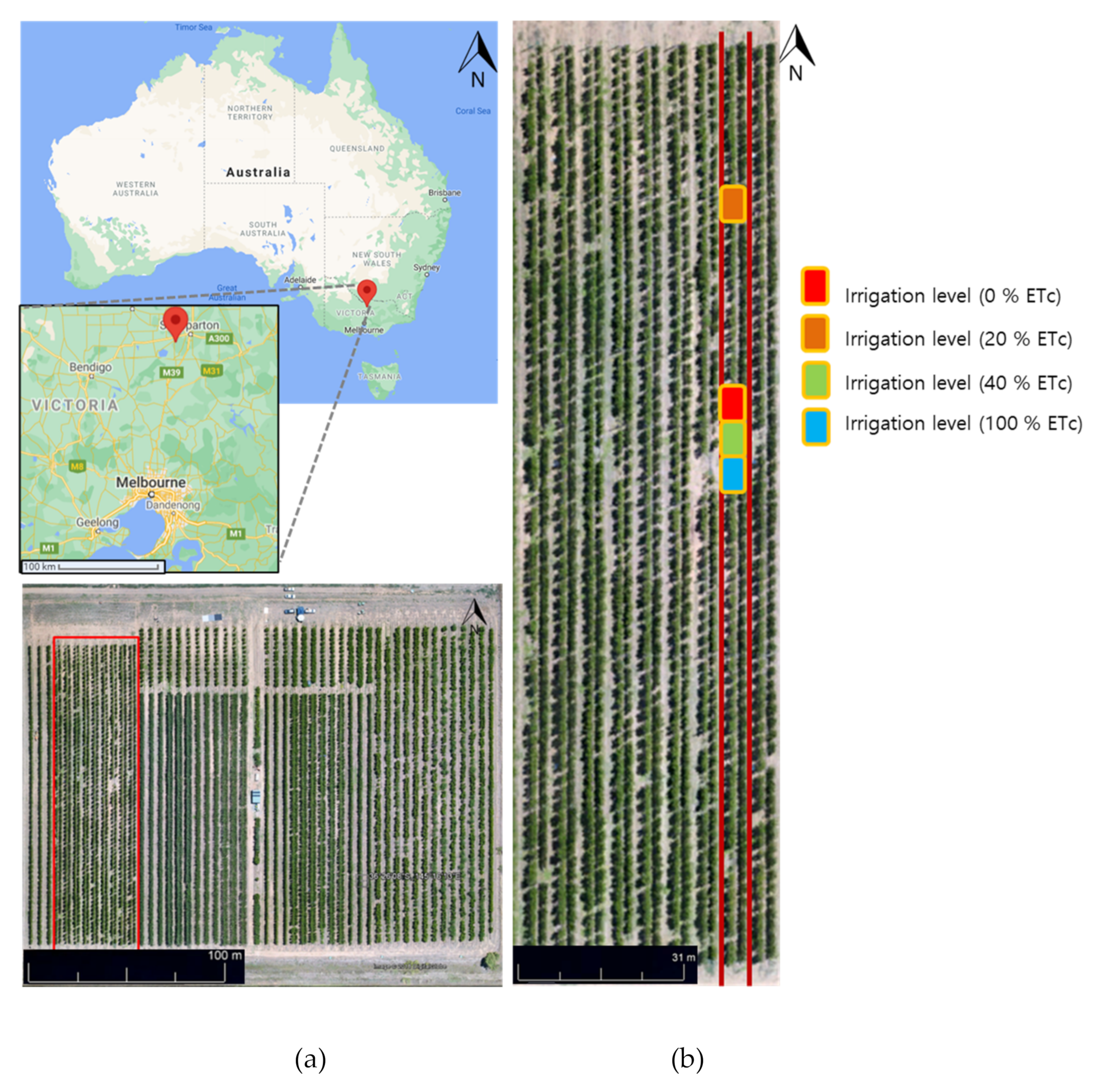
2.1. Study Site Description

The experimental site is a nectarine orchard (0.7 ha, 150 m × 45 m), located near Tatura, Victoria, Australia (36°26′08” S, 145°16′13” E, 114 m AMSL). The Stonefruit Experimental Orchard, Tatura SmartFarm is administered by the Department of Jobs, Precincts and Regions. The climate of Tatura is temperate. The annual average reference crop evapotranspiration is 1190 mm, and the annual precipitation is 480 mm in the region. The site was planted in 2014 with a nectarine called ‘September Bright’ on an Open Tatura training system (tree height 2.0 m, tree spacing 1.0 m). The nectarine fruit was in stage III of fruit maturity with the tree canopy under midseason full leaf-up. The Open Tatura (OT) is V-shaped with two trellis arms, designed to increase light interception and provide more uniform light distribution for high marketable yields. The trees are planted in a north-south direction on a fine, sandy, loamy, Shepparton soil. The tree- and inter-row spacing is 1.0 m and 4.5 m, respectively (2,222 trees/ha).

The study site used a subset of the entire orchard irrigation experiment, focusing on four experimental plots in close proximity (Figure 1), where four different irrigation levels were applied as control (W4_100) and water deficit treatments (W1_20, W2_0, and W3_40), as shown in

Table 1. Summary of irrigation levels applied to control and treatment plots.

Plot ID	Cultivar	Treatment	Irrigation Level
W1_20	Nectarine	Deficit	20 % ETc
W2_0		Deficit	0 % ETc
W3_40		Deficit	40 % ETc
W4_100		Control	100 % ETc

. Experimental layout of plots was a randomized block design. Blocks of sampling trees were selected randomly and treated with designated deficit irrigations.

The orchard was drip-irrigated daily, and the irrigation amount was calculated by a weather-based ETc (crop evapotranspiration) model by FAO-56 approach [33]. A crop coefficient of ETc was adjusted for tree size, by measuring fractional photosynthetically active radiation (fPAR) interception [34]. The irrigation amount was controlled daily via a single drip line comprising of in-line pressure compensated emitters (1.6 l/h discharge, 0.5 m spacing). Each plot of control and water deficit treatments contained three adjacent rows of eighteen trees to adequately delimit the treatments. The middle three trees in each plot were used for field and remote sensing measurements.

2.2. Data Acquisition

Three UAV flights were conducted on the 19 January 2017. The aerial TIR imagery was acquired from morning to afternoon distributed at 9 h, 12 h, and 15 h solar time. The experimental day was with a clear sky, moderate winds (0.6 m sec⁻¹), air temperature around 30.6 °C and relative humidity 26.7 % at midday, measured from the nearby (<200 m) meteorological station. The weather condition of each time of UAV campaign is shown in

Table 2. Weather conditions at three times of data acquisition on 19 January 2017, Tatura.

Acquisition Time of Data	Air Temperature	Relative Humidity	Wind Speed
9 h	26.8 °C	34.7 %	0.9 m s−1
12 h	30.6 °C	26.7 %	0.6 m s−1
15 h	33.2 °C	18.8 %	1.2 m s−1

.

A TIR camera (A65, FLIR Systems, Inc., Wilsonville, OR, USA) was integrated with a GPS and an onboard computer for geo-tagging and mounted to a multi-rotor UAV platform (S1000, DJI, Shenzhen, China). TIR images were captured in the spectral wavelength of 7.5–13 µm, a spatial resolution of 640 × 512 pixels, a focal length of 25 mm, and a FOV of 25° (H) × 20° (V).

All aerial images from the TIR sensor were taken within a short time window (< 10 min) to minimize the temporal variation of canopy temperature during the flight over the site. The TIR camera was mounted to a high-performance gimbal to enable stable image acquisition at nadir view. The UAV was flown at an altitude of 90 m above ground level (AGL) to capture images with an overlap of 80 % forward and 40 % side, respectively, by an autonomous flight plan. The footprint of a TIR image is 39 m × 31 m with a ground sample distance (GSD) of 6 cm.

During the UAV sensing, two types of calibration targets were deployed at the site: (1) temperature calibration target for TIR images and; (2) ground control point (GCP) and ground artificial feature (GAF) for image orthomosaicking. The water body and rubber plates were deployed for calibration targets of TIR images as cold and hot features with high emissivity. The specific GCP target was designed for performing an accurate and robust orthomosaicking and GAF targets were designed for increasing key points available for the photogrammetric matching process presented in previous research [19]. The GCP target was made of an aluminium plate with a black cross (0.6 m × 0.6 m size) and surveyed by a differential GPS (DGPS) with higher than 3 cm positional accuracy. The GAF targets were made of aluminium-coated cardboard with three shapes: triangle, trapezoid, and rectangle. Both targets were distinctively presented as a cold temperature in thermal images due to a low emissivity of aluminium material.

With each UAV flight, the measurements of crop physiological data were carried out at the irrigation treatment plots simultaneously of aerial image acquisition. Gas exchange measurements using a photosynthesis system (LI-6400, LI-COR Inc., Lincoln, Nebraska, USA) were conducted on fully expanded leaves (n = 6 leaves × 4 plots = 24 observations) to obtain stomatal conductance (g_s, mmol m⁻² sec⁻¹) at 9 h, 12 h and 15 h. Leaf temperature was measured on both sunlit and shaded leaves (n = 10 leaves × 4 plots = 40 observations) using a thermometer (TN410LCE, ZyTemp, Radiant Innovation Inc., Hsinchu City, Taiwan). Midday stem water potential (ψ_stem, MPa) was measured on two fully expanded shaded leaves per tree in each plot (n = 4 leaves × 4 plots = 16 observations) using a Scholander pressure chamber (Model 3000, Soil Moisture Equipment Co., Santa Barbara, CA, USA). The leaves were selected from branches near the main trunk and were covered with an aluminium foil bag for a minimum of one hour of equilibration time before the measurement of ψ_stem.

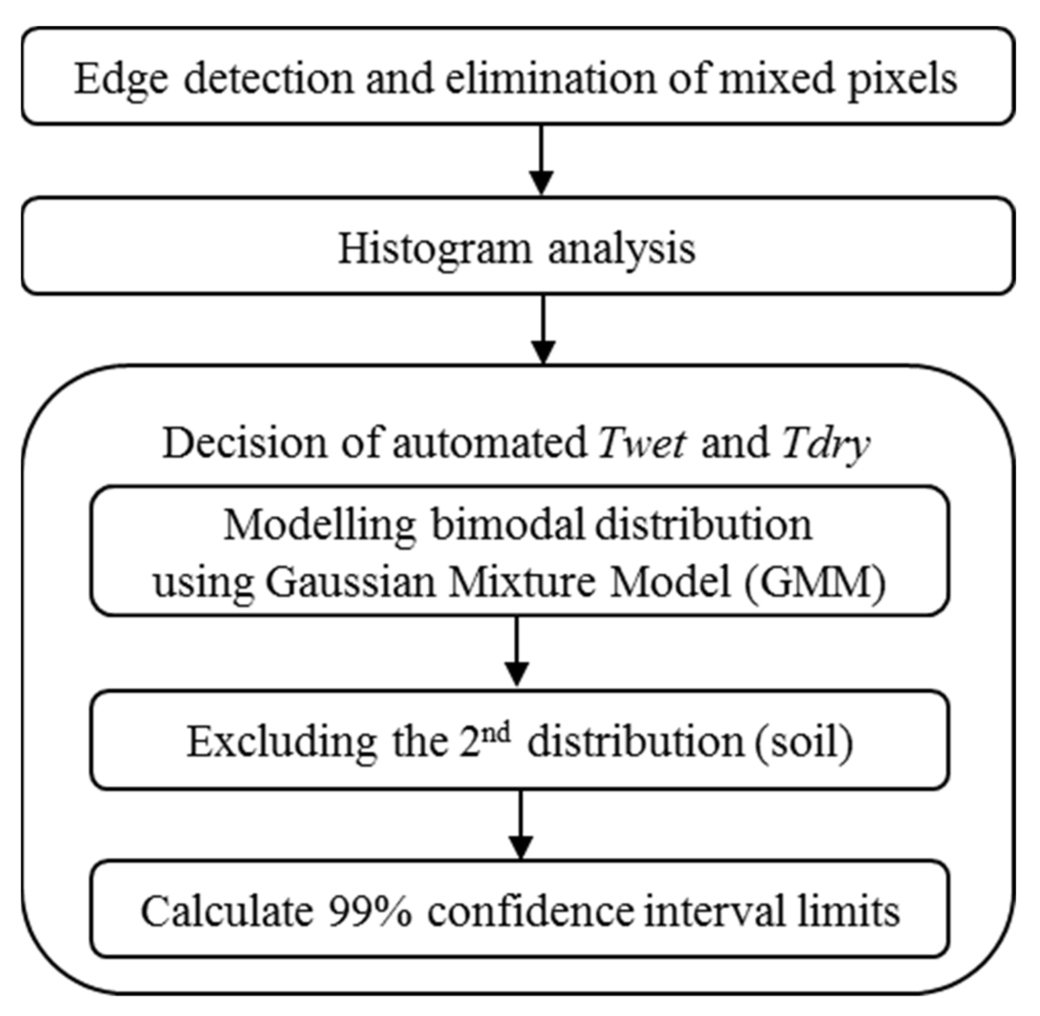
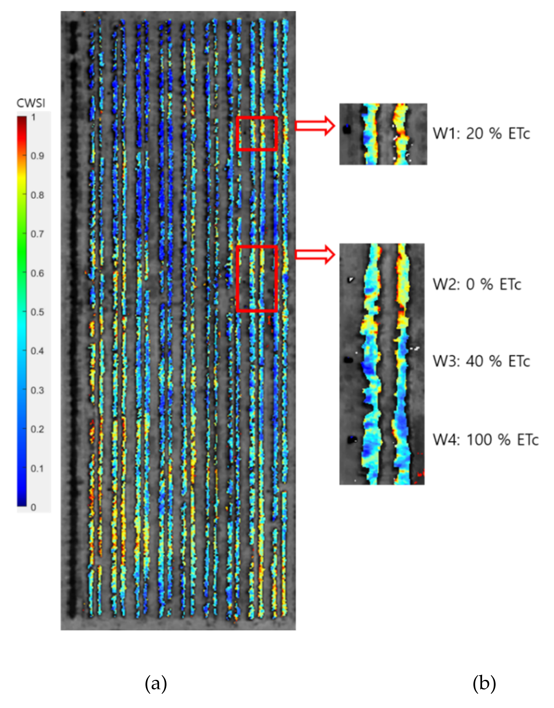
2.3. TIR Image Processing

Based on the method of Adaptive CWSI estimation proposed in the previous research [19], all aerial TIR images were processed to estimate plant water stress at each time: 9 h, 12 h and 15 h.

Temperature calibration of thermal images was carried out to retrieve accurate plant temperatures with a known temperature from calibration targets. As a method, the raw signal-format TIR images were converted to temperature-based images using a one-point calibration by the FLIR Systems [35], as shown in Equations (1) and (2). When correlating the signal to the temperature, the calibration targets made of rubber sheets and water bodies were used to refer to the actual temperatures as hot and cold features. The TIR snapshot measured the target temperatures by a handheld thermal imaging camera (T640, FLIR Systems, Inc., Wilsonville, OR, USA) and a handheld thermometer concurrently with the UAV flight. The temperature of the calibration target was used to calculate the adjusted offset parameter ($O_{adjusted}$) (Equation 1), and then adjusted temperature was obtained (Equation 2):

$$O_{adjusted}=S-\frac{R}{e^{\left(B/T_{known}in Kelvin\right)-1}}$$

(1)

$$T_{adjusted \left(in Kelvin\right)}=\frac{B}{\log \left(\frac{R}{S-O_{adjusted}}+1\right)}$$

(2)

where S is a 14-bit raw signal value, T an object temperature, R a constant for converting flux to temperature derived from Planck’s constant h, B a constant derived from Boltzmann’s constant and Planck’s constant h, O an offset (signal to radiance).

All calibrated TIR images were stitched into a georeferenced image using photogrammetric software (PhotoScan, Agisoft LLC, St. Petersburg, Russia).

For the extraction of pure canopy pixels from the imagery, the mixed pixels (edges) along the boundary between canopy and soil pixels were detected by the combined Sobel and Canny technique in Matlab R2014b. The detected edges were dilated for more conservative exclusion of the mixed pixels and removed from the original orthomosaic image.

2.4. Plant Water Stress Modelling Using Adaptive CWSI Method

The concept of CWSI was used to interpret the level of plant water stress by the normalization of the difference between canopy temperature of the plant ($T_c$) and reference temperatures, where reference implies fully transpiring ($T_{wet}$) and non-transpiring leaf ($T_{dry}$). The CWSI formula is presented as follows [5]:

$$CWSI=\frac{T_c-T_{wet}}{T_{dry}-T_{wet}}$$

(3)

The Adaptive CWSI in an earlier research was proposed to determine site-cultivar dependency, specifically for reference temperatures based on statistical analysis. This new method addressed an adaptive approach of CWSI estimation in two aspects: (1) Finding that the behaviour of canopy temperature was different from cultivar type and canopy structure even under the identical irrigation regime. Thus, the new Adaptive CWSI method, employing single reference boundary of T_wet and T_dry, could not accommodate to such behaviour. Thus, the adaptive CWSI with multiple reference boundaries of T_wet and T_dry was proposed by classifying the region into sub-regions of the same crop property. (2) Determining automatic thresholds of T_wet and T_dry by a statistical approach using the Gaussian mixture modelling (GMM). In this way, Adaptive CWSI hypothesised that T_wet and T_dry can be obtained at two extremes in the distribution of canopy temperatures under the assumption of the presence of water-stressed and non-water-stressed plants in the region analysed. Mixed pixels of canopy and non-canopy were discarded to obtain pure canopy distribution for the temperature histogram, by adopting the method of edge detection and extraction.

Figure 2 describes the process work flow for Adaptive CWSI estimation. In this research, the temperature histogram was generated from the edge-free TIR image to analyze the temperature distribution statistically. Since the study site has a single cultivar (nectarine) with the same canopy structure (Open Tatura), the site was treated as one property. Thus, the classification of sub-regions was not required for the site. The GMM was fitted to the temperature distribution to separate canopy and soil pixels in distinctive bimodal and normal density distributions and to estimate the reference boundary values, T_wet and T_dry, for the CWSI estimation. The higher-temperature component (2^nd distribution) of the Gaussian distribution, representing soil pixels, was removed to exclude non-canopy samples. Then, the adaptive threshold of T_wet and T_dry was automatically determined by sampling 0.5 and 99.5 percentile values from the canopy-temperature component (1^st distribution) of Gaussian distribution. The critical value of 99% confidence interval limits was derived empirically from the previous research [19], assigning the coldest and hottest temperatures as T_wet and T_dry, respectively.

3. Results

3.1. Relationship of CWSI with Midday Stem Water Potential

Figure 3a shows the estimated CWSI map based on adaptive of T_wet and T_dry derived from the midday UAV flight. The water stress variability over the orchard is visually presented in the CWSI map. Figure 3b shows the details of four experimental plots in water deficit and control treatment groups: W1_20, W2_0, W3_40 and W4_100.

CWSI values of trees from each experimental plot were extracted and averaged from the CWSI map to show the representative CWSI value for each plot. The CWSI values in all four irrigation groups exhibited a strong negative correlation with the midday ψ_stem, with determination coefficients (R²) of 0.83 (Figure 4). In W1_20 and W2_0 plots, high-water-stress treatments were applied; subsequently, the measured ψ_stem of each plot indicated water deficit condition with a similar value of −2.6 MPa and −2.8 MPa, respectively. The ψ_stem values for W3_40 and W4_100 were also shown in close range with values of −1.7 MPa and −1.6 MPa, respectively, representing low-water-stress condition. All ψ_stem from W1–W4 plots were measured with standard deviations (SDs) of 0.11, 0.06, 0.28 and 0.21 MPa, respectively.

Similar results were obtained for the estimated CWSI. The CWSIs in W1_20 and W2_0 were estimated in the equivalent values (approx. 0.66 and 0.60, respectively), and were higher than in W3_40 and W4_100 (approx. 0.49 and 0.44, respectively). CWSIs from W1–W4 plots were obtained with SDs of 0.07, 0.04, 0.09 and 0.07, respectively.

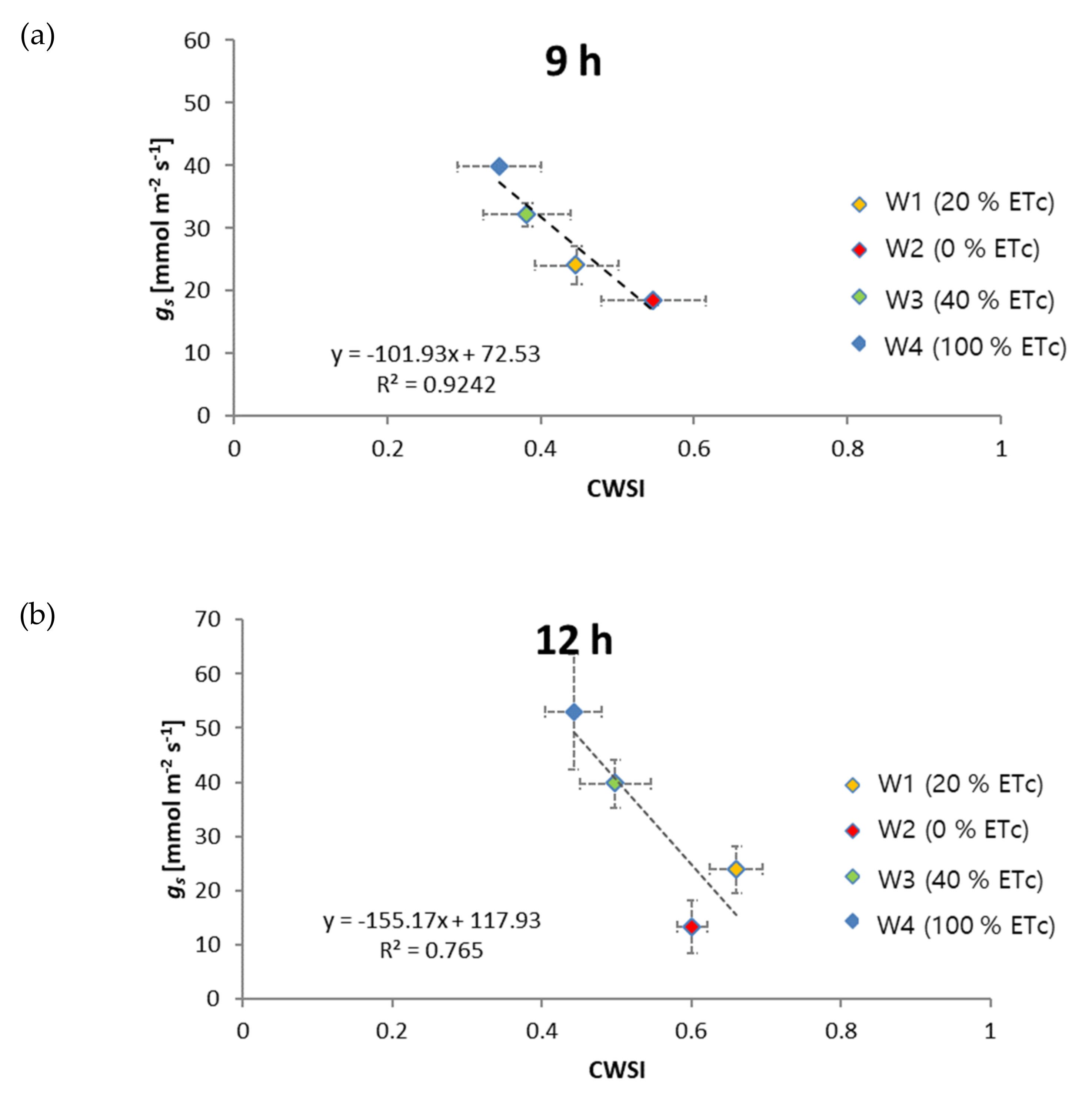
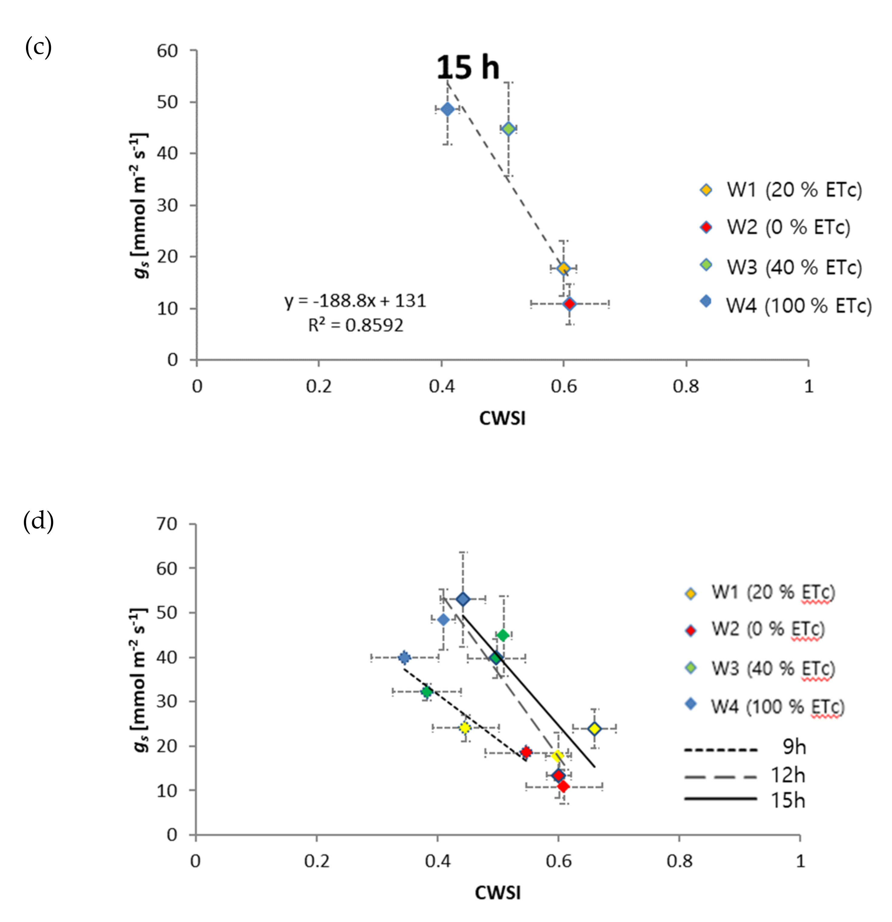
3.2. Relationship of CWSI with Diurnal Plant Water Stress

The difference between canopy and air temperature (T_c – T_a) was also measured at three times of the day. Figure 5 shows T_c – T_a of control plot (W4_100) and deficit plot (W2_0) from morning to afternoon. The canopy-air temperature difference T_c – T_a changed considerably during the day in both irrigation treatment plots, starting positive and becoming negative T_c – T_a. In the morning (9 h), the canopy temperature was higher than the air temperature since the canopy was becoming warm. At midday, canopy temperature was becoming cooler than air in the control plot. The latter is considered to be due to transpiration cooling. T_c – T_a approached zero in the case of deficit plot, indicating higher canopy temperature than control plot, which was derived from water stress. Overall, the water deficit plot (W2_0) resulted in higher canopy temperature than the fully irrigated plot (W4_100) during three measurements (≈ 3 °C), related to typical daily depression.

Stomatal conductance (g_s) measurements were used to provide the relationships with the estimated CWSIs at different times of the day, as shown in Figure 6.

Similarly, with midday ψ_stem, a strong relationship was found between g_s measurements and the adaptive CWSI at 9 h, 12 h, and 15 h. Specifically, the relationship of each time was significant with determination coefficients (R²) of 0.92, 0.77 and 0.86, respectively.

From the results at 9h in Figure 6, the measured g_s from each plot showed a gradual increase of values according to the irrigation level with g_s values from 18.4 (mmol m⁻² sec⁻¹) at W2_0 to 39.8 (mmol m⁻² sec⁻¹) at W4_100. Inversed results were found for the estimated CWSI, showing that the CWSI values gradually dropped with a higher irrigation level. In Figure 6, the relationships presented were derived from midday and afternoon. Both CWSIs were significantly correlated with g_s measurements.

In the diurnal variation of plant water stress, morning g_s showed less variation than midday and afternoon g_s over all the irrigation regimes (0, 20, 40 and 100 % ETc), as shown in

Table 3. Statistics of the extreme gs over all irrigation regimes at three times of the day.

Acquisition Time	SD of Extreme gs (mmol m−2 sec−1)	Mean of Extreme gs (mmol m−2 sec−1)	Size of Extreme gs (%)
9 h	9.35	28.61	32.7
12 h	17.46	32.48	53.8
15 h	18.98	30.46	62.3

SD: Standard Deviation.

. However, the distribution of g_s, which is the difference of extreme g_s in 0 % ETc and 100 % ETc, became significantly wider from morning to midday, remaining at a similar scale (slightly wider) from midday to afternoon. Results showed a reduction of the range of of the distribution of morning g_s compared to midday and afternoon values, which is a typical regulation of g_s induced by photosynthetic rate in the morning [36]. However, results also showed that all g_s values were highly correlated to water-stressed levels (Figure 6).

In the water-stressed plots, the g_s of W1_20 and W2_0 responded at the rates of 18–24 (mmol m⁻² sec⁻¹) at 9 h. Then, the g_s of W1_20 and W2_0 slightly decreased and remained at 13–24 (mmol m⁻² sec⁻¹) at 12 h. Then, g_s of W1_20 and W2_0 considerably dropped to 11–17 (mmol m⁻² sec⁻¹) at 15 h. The response of g_s in water-stressed plants can indicate that stomatal conductance decreases due to the stomatal closure and less transpiration during daytime.

In the control plot (W4_100), g_s showed higher rates than other deficit irrigation plots at three times of the day. Particularly, midday g_s was obtained at the highest rate, 53 (mmol m⁻² sec⁻¹).

Overall, midday and afternoon g_s were measured at a similar range, while morning g_s displayed a lower conductance rate than midday and afternoon periods. However, in water deficit plots, midday and afternoon g_s responded at lower rates than morning g_s, indicating that the water-stressed plant behaves with more limited stomatal conductance during periods of higher evaptorative demand.

4. Discussion

This research explored the behaviour of daytime CWSIs and a plant physiological parameter (g_s) in water deficit irrigation regimes. In general, the magnitude of g_s had a negative linear relationship with respect to the plant water stress level at three times of measurement.

The estimated CWSIs taken at three times of the day showed a significant correlation with g_s according to the irrigation levels. Unlike the variation of the extreme g_s throughout the day, CWSIs remained in a similar range of the extreme values at each flight time, as shown in

Table 4. Statistics of the extreme adaptive CWSI over all the irrigation regimes at three times of the day.

Acquisition Time	SD of Extreme CWSI	Mean of Extreme CWSI	Size of Extreme CWSI
9 h	0.088	0.43	20.5 %
12 h	0.098	0.55	17.9 %
15 h	0.093	0.53	17.5 %

SD: Standard Deviation.

. The morning CWSI was slightly lower (0.11 of CWSI) than midday and afternoon CWSIs; a similar trend was visible in morning g_s (Figure 6 and Table 4).

The canopy temperature difference from the extreme irrigation plots (W2_0 and W4_100) was 2.6 °C. Previous CWSI studies based on VPD and air temperature to calculate T_wet and T_dry (or baselines) have shown that the CWSI calculation for morning periods is challenging and fails to determine the baseline due to a narrow range of temperature differences between the upper and lower baselines (e.g., 2 °C) [26]. As the Adaptive CWSI method relies on statistical modelling of canopy temperatures, T_wet and T_dry can be obtained at two extremes in the distribution of canopy temperatures under the assumption of the presence of water decifit and control plants in the region. Thus, the CWSI method can obtain T_wet and T_dry in the small range of temperature differences, making it more sensitive. As a result, morning CWSI was estimated at a reliable level to interpret plant water stress. This research also found that the estimated CWSIs were incorporated according to magnitude of g_s during the day, since the size of CWSI range was obtained at a similar scale at each time of the day. The latter could imply that Adaptive CWSIs enable different water-stressed plants with high sensitivity and consistent scale from morning to afternoon within the same day. Nevertheless, the range of Adaptive CWSI can be biased in terms of absolute quantity due to the limitation of the statistical histogram approach, as described in [19], since the Adaptive CWSI method has the assumption that a wide range of water stress levels are presented in fields. However, the bias can be adjusted by a simple relationship between CWSI and irrigation. It remains a practical method to estimate CWSI across an area during the day.

5. Conclusions

This study analyzed the diurnal changes of plant water stress using: 1) plant physiological data—stomatal conductance (g_s) and stem water potential (ψ_stem); and 2) estimated CWSI derived from TIR UAV sensing at three different times of the day: 9 h, 12 h and 15 h. In addition, this study tested the method’s performance in estimating the diurnal behaviour of water stress in the different deficit irrigation regimes.

The estimation was performed by adopting the method of Adaptive CSWI. Significant relationships between CWSI and g_s (and ψ_stem) were found at each flight time of the day. Thus, the adaptive CWSI method showed a capability to interpret plant water stress levels even with the small range of boundary limits in the morning. Particularly, morning CWSI presented a relative consistency with midday and afternoon CWSI. Thus, the present research can potentially provide any daytime CWSI estimations since they can be estimated accurately with low contrast of surface temperatures from late morning to late afternoon. Subsequently, the method can assist in extending the time window of UAV remote sensing during the day. In addition, the Adaptive CWSIs estimated from UAV thermal sensing can provide a practical method to assess the spatially heterogeneous distribution of water stress within plants at a sub-field scale for precision irrigation management. The method proposed can also feasibly be applied for interpreting plant water stress since it requires only thermal imagery as an input. The boundary limits of CWSI estimation are automatically determined by probability modelling.

The research presented, however, was conducted in a single nectarine cultivar in the summertime. Thus, various crop-cultivar-site- and time-specific experiments will remain for future work that can use the full advantages of the Adaptive CWSI method. Future research could show the extent to which the presented approaches are applicable for precision agriculture.

References

1. Davies, F.S.; Lakso, A.N. Diurnal and Seasonal Changes in Leaf Water Potential Components and Elastic Properties in Response to Water Stress in Apple Trees. Physiol. Plant. 1979, 46, 109. [Google Scholar] [CrossRef]
2. Williams, L.E.; Araujo, F.J. Correlations among predawn leaf, midday leaf, and midday stem water potential and their correlations with other measures of soil and plant water status in Vitis vinifera. J. Am. Soc. Hortic. Sci. 2002, 127, 448–454. [Google Scholar] [CrossRef] [Green Version]
3. Bhusal, N.; Bhusal, S.J.; Yoon, T.-M. Comparisons of physiological and anatomical characteristics between two cultivars in bi-leader apple trees (Malus × domestica Borkh.). Sci. Hortic. 2018, 231, 73–81. [Google Scholar] [CrossRef]
4. Poblete-Echeverría, C.; Espinace, D.; Sepúlveda-Reyes, D.; Zúñiga, M.; Sanchez, M. Analysis of crop water stress index (CWSI) for estimating stem water potential in grapevines: Comparison between natural reference and baseline approaches. ActaHortic. 2017, 1150, 189–194. [Google Scholar] [CrossRef]
5. Jones, H.G. Plants and Microclimate: A Quantitative Approach to Environmental Plant Physiology; Cambridge University Press: New York, NY, USA, 1992. [Google Scholar]
6. Alchanatis, V.; Cohen, Y.; Cohen, S.; Moller, M.; Sprinstin, M.; Meron, M.; Tsipris, J.; Saranga, Y.; Sela, E. Evaluation of different approaches for estimating and mapping crop water status in cotton with thermal imaging. Precis. Agric. 2010, 11, 27–41. [Google Scholar] [CrossRef]
7. Blaya-Ros, P.J.; Blanco, V.; Domingo, R.; Soto-Valles, F.; Torres-Sánchez, R. Feasibility of Low-Cost Thermal Imaging for Monitoring Water Stress in Young and Mature Sweet Cherry Trees. Appl. Sci. 2020, 10, 5461. [Google Scholar] [CrossRef]
8. Testi, L.; Goldhamer, D.A.; Iniesta, F.; Salinas, M. Crop water stress index is a sensitive water stress indicator in pistachio trees. Irrig. Sci. 2008, 26, 395–405. [Google Scholar] [CrossRef] [Green Version]
9. Bellvert, J.; Zarco-Tejada, P.; Girona, J.; Fereres, E. Mapping crop water stress index in a ’Pinot-noir’ vineyard: Comparing ground measurements with thermal remote sensing imagery from an unmanned aerial vehicle. Precis. Agric. 2014, 15, 361–376. [Google Scholar] [CrossRef]
10. Nagai, M.; Chen, T.; Shibasaki, R.; Kumagai, H.; Ahmed, A. UAV-Borne 3-D Mapping System by Multisensor Integration. IEEE Trans. Geosci. Remote. Sens. 2009, 47, 701–708. [Google Scholar] [CrossRef]
11. Yao, H.; Qin, R.; Chen, X. Unmanned Aerial Vehicle for Remote Sensing Applications—A Review. Remote. Sens. 2019, 11, 1443. [Google Scholar] [CrossRef] [Green Version]
12. Gómez-Candón, D.; Virlet, N.; Labbé, S.; Jolivot, A.; Regnard, J.-L. Field phenotyping of water stress at tree scale by UAV-sensed imagery: New insights for thermal acquisition and calibration. Precis. Agric. 2016, 17, 786–800. [Google Scholar] [CrossRef]
13. Hoffmann, H.; Jensen, R.; Thomsen, A.; Nieto, H.; Rasmussen, J.; Friborg, T. Crop water stress maps for an entire growing season from visible and thermal UAV imagery. Biogeosciences 2016, 13, 6545–6563. [Google Scholar] [CrossRef] [Green Version]
14. Zhang, L.; Niu, Y.; Zhang, H.; Han, W.; Li, G.; Tang, J.; Peng, X. Maize Canopy Temperature Extracted From UAV Thermal and RGB Imagery and Its Application in Water Stress Monitoring. Front. Plant Sci. 2019, 10, 1270. [Google Scholar] [CrossRef]
15. Gago, J.; Douthe, C.; Coopman, R.E.; Gallego, P.P.; Ribas-Carbo, M.; Flexas, J.; Escalona, J.; Medrano, H. UAVs challenge to assess water stress for sustainable agriculture. Agric. Water Manag. 2015, 153, 9–19. [Google Scholar] [CrossRef]
16. Patrick, A.; Pelham, S.; Culbreath, A.; Holbrook, C.C.; Godoy, I.J.D.; Li, C. High throughput phenotyping of tomato spot wilt disease in peanuts using unmanned aerial systems and multispectral imaging. IEEE Instrum. Meas. Mag. 2017, 20, 4–12. [Google Scholar] [CrossRef]
17. Delavarpour, N.; Koparan, C.; Nowatzki, J.; Bajwa, S.; Sun, X. A Technical Study on UAV Characteristics for Precision Agriculture Applications and Associated Practical Challenges. Remote. Sens. 2021, 13, 1204. [Google Scholar] [CrossRef]
18. Crusiol, L.G.T.; Nanni, M.R.; Furlanetto, R.H.; Sibaldelli, R.N.R.; Cezar, E.; Mertz-Henning, L.M.; Nepomuceno, A.L.; Neumaier, N.; Farias, J.R.B. UAV-based thermal imaging in the assessment of water status of soybean plants. Int. J. Remote. Sens. 2020, 41, 3243–3265. [Google Scholar] [CrossRef]
19. Suyoung, P.; Dongryeol, R.; Fuentes, S.; Hoam, C.; Hernández-Montes, E.; O’Connell, M. Adaptive Estimation of Crop Water Stress in Nectarine and Peach Orchards Using High-Resolution Imagery from an Unmanned Aerial Vehicle (UAV). Remote. Sens. 2017, 9, 1–15. [Google Scholar]
20. Poblete, T.; Ortega-Farías, S.; Ryu, D. Automatic Coregistration Algorithm to Remove Canopy Shaded Pixels in UAV-Borne Thermal Images to Improve the Estimation of Crop Water Stress Index of a Drip-Irrigated Cabernet Sauvignon Vineyard. Sensors 2018, 18, 397. [Google Scholar] [CrossRef] [PubMed] [Green Version]
21. Gago, J.; Fernie, A.R.; Nikoloski, Z.; Tohge, T.; Martorell, S.; Escalona, J.M.; Ribas-Carbó, M.; Flexas, J.; Medrano, H. Integrative field scale phenotyping for investigating metabolic components of water stress within a vineyard. Plant. Methods 2017, 13, 90. [Google Scholar] [CrossRef]
22. Poblete, T.; Ortega-Farías, S.; Moreno, M.A.; Bardeen, M. Artificial Neural Network to Predict Vine Water Status Spatial Variability Using Multispectral Information Obtained from an Unmanned Aerial Vehicle (UAV). Sensors 2017, 17, 2488. [Google Scholar] [CrossRef] [PubMed] [Green Version]
23. Millán, S.; Campillo, C.; Vivas, A.; Moñino, M.J.; Prieto, M.H. Evaluation of Soil Water Content Measurements with Capacitance Probes to Support Irrigation Scheduling in a “Red Beaut” Japanese Plum Orchard. Agronomy 2020, 10, 1757. [Google Scholar] [CrossRef]
24. Naor, A. Midday stem water potential as a plant water stress indicator for irrigation scheduling in fruit trees. ActaHortic. 2000, 357, 447–454. [Google Scholar] [CrossRef]
25. Fernández, J.E. Plant-Based Methods for Irrigation Scheduling of Woody Crops. Horticulturae 2017, 3, 35. [Google Scholar] [CrossRef] [Green Version]
26. Gonzalez-Dugo, V.; Zarco-Tejada, P.; Nicolás, E.; Nortes, P.; Alarcón, J.; Intrigliolo, D.; Fereres, E. Using high resolution UAV thermal imagery to assess the variability in the water status of five fruit tree species within a commercial orchard. Precis. Agric. 2013, 14, 660–678. [Google Scholar] [CrossRef]
27. Micol, R.; Cinzia, P.; Chiara, C.; Michele, M.; Lorenzo, B.; Sergio, C.; Stefano, A.; Roberto, C. Discriminating irrigated and rainfed maize with diurnal fluorescence and canopy temperature airborne maps. ISPRS Int. J. Geo Inform. 2015, 4, 626–646. [Google Scholar]
28. Martínez, J.; Egea, G.; Agüera, J.; Pérez-Ruiz, M. A cost-effective canopy temperature measurement system for precision agriculture: A case study on sugar beet. Precis. Agric. 2017, 18, 95–110. [Google Scholar] [CrossRef]
29. Casas-Mulet, R.; Pander, J.; Ryu, D.; Stewardson, M.J.; Geist, J. Unmanned Aerial Vehicle (UAV)-Based Thermal Infra-Red (TIR) and Optical Imagery Reveals Multi-Spatial Scale Controls of Cold-Water Areas Over a Groundwater-Dominated Riverscape. Front. Environ. Sci. 2020, 8, 64. [Google Scholar] [CrossRef]
30. Jackson, R.D.; Idso, S.B.; Reginato, R.J.; Pinter, P.J., Jr. Canopy temperature as a crop water stress indicator Wheat. Water Resour. Res. 1981, 17, 1133–1138. [Google Scholar] [CrossRef]
31. Jones, H.G. Use of infrared thermometry for estimation of stomatal conductance as a possible aid to irrigation scheduling. Agric. For. Meteorol. 1999, 95, 139–149. [Google Scholar] [CrossRef]
32. Möller, M.; Alchanatis, V.; Cohen, Y.; Meron, M.; Tsipris, J.; Naor, A.; Ostrovsky, V.; Sprintsin, M.; Cohen, S. Use of thermal and visible imagery for estimating crop water status of irrigated grapevine. J. Exp. Bot. 2007, 58, 827–838. [Google Scholar] [CrossRef] [PubMed] [Green Version]
33. Allen, R.G.; Pereira, L.S.; Raes, D.; Smith, M. Crop Evapotranspiration: Guidelines for computing crop water requirements. FAO Irrig. Drain. Pap. 1998, 300, D05109. [Google Scholar]
34. Scalisi, A.; O’Connell, M.G.; Stefanelli, D.; Lo Bianco, R. Fruit and Leaf Sensing for Continuous Detection of Nectarine Water Status. Front. Plant Sci. 2019, 10, 805. [Google Scholar] [CrossRef] [PubMed] [Green Version]
35. FLIRSystems. User’s Manual FLIR Ax5 Series; T559770; FLIR Systems: Wilsonville, OR, USA, 2013. [Google Scholar]
36. Whitehead, D. Regulation of stomatal conductance and transpiration in forest canopies. Tree Physiol. 1998, 18, 633–644. [Google Scholar] [CrossRef] [PubMed]
Figure 1. (a) Study site location, Stonefruit Experimental Orchard (Tatura, Victoria, Australia). (b) Different levels of water deficit plots are presented in red (0 % ETc), orange (20 % ETc), green (40 % ETc), and blue (100 % ETc) zones.
Remotesensing 13 02775 g001
Figure 2. Flowchart of the analysis steps for CWSI estimation based on adaptive reference baselines.
Remotesensing 13 02775 g002
Figure 3. (a) Adaptive CWSI map derived from midday UAV remote sensing for the entire experimental nectarine orchard, Tatura. The red rectangles represent the area of irrigation treatments. (b) Detailed adaptive CWSI map depicting the experimental plots of W1 (20 % ETc), W2 (0 % ETc), W3 (40 % ETc) and W4 (100 % ETc).
Remotesensing 13 02775 g003
Figure 4. Relationship between midday stem water potential and adaptive CWSI at 12 h.
Remotesensing 13 02775 g004
Figure 5. Differences between canopy and air temperature at three times of the day in control (100% ETc) and deficit (0% ETc) plots.
Remotesensing 13 02775 g005
Figure 6. Relationships between stomatal conductance (gs) and adaptive CWSI acquired at: (a) 9 h; (b) 12 h; (c) 15 h; and (d) all three times.
Remotesensing 13 02775 g006aRemotesensing 13 02775 g006b