Rapid Single Image-Based DTM Estimation from ExoMars TGO CaSSIS Images Using Generative Adversarial U-Nets

Abstract

The lack of adequate stereo coverage and where available, lengthy processing time, various artefacts, and unsatisfactory quality and complexity of automating the selection of the best set of processing parameters, have long been big barriers for large-area planetary 3D mapping. In this paper, we propose a deep learning-based solution, called MADNet (Multi-scale generative Adversarial u-net with Dense convolutional and up-projection blocks), that avoids or resolves all of the above issues. We demonstrate the wide applicability of this technique with the ExoMars Trace Gas Orbiter Colour and Stereo Surface Imaging System (CaSSIS) 4.6 m/pixel images on Mars. Only a single input image and a coarse global 3D reference are required, without knowing any camera models or imaging parameters, to produce high-quality and high-resolution full-strip Digital Terrain Models (DTMs) in a few seconds. In this paper, we discuss technical details of the MADNet system and provide detailed comparisons and assessments of the results. The resultant MADNet 8 m/pixel CaSSIS DTMs are qualitatively very similar to the 1 m/pixel HiRISE DTMs. The resultant MADNet CaSSIS DTMs display excellent agreement with nested Mars Reconnaissance Orbiter Context Camera (CTX), Mars Express’s High-Resolution Stereo Camera (HRSC), and Mars Orbiter Laser Altimeter (MOLA) DTMs at large-scale, and meanwhile, show fairly good correlation with the High-Resolution Imaging Science Experiment (HiRISE) DTMs for fine-scale details. In addition, we show how MADNet outperforms traditional photogrammetric methods, both on speed and quality, for other datasets like HRSC, CTX, and HiRISE, without any parameter tuning or re-training of the model. We demonstrate the results for Oxia Planum (the landing site of the European Space Agency’s Rosalind Franklin ExoMars rover 2023) and a couple of sites of high scientific interest.

1. Introduction

The Martian surface shows many distinct morphological features that have been formed by different types of geological processes over its ancient history. These processes, involving volcanism, tectonism, water and aeolian erosion, dust deposition, changes in the polar ice caps, and hypervelocity impact cratering, have shaped the planet on a global and local scale. Three-dimensional (3D) reconstruction and modelling using remotely, or locally sensed optical images are usually the necessary first step to studying such surface processes of the Martian surface.

There has been a revolution in Martian 3D surface studies over the last 18 years, since the first stereo photogrammetric imaging data acquired by the Mars Express’s High Resolution Stereo Camera (HRSC) at 12.5 m/pixel in January 2004 [1], which was designed to be used for high-resolution 3D mapping. Over that time, the resolution of orbital imagery has improved from tens of metres per pixel down to 25 cm/pixel with different swath width. These include images from the Mars Reconnaissance Orbiter (MRO) Context Camera (CTX) at 6 m/pixel [2], MRO High Resolution Imaging Science Experiment (HiRISE) at 25 cm/pixel [3], and more recently, the ExoMars Trace Gas Orbiter (TGO) Colour and Stereo Surface Imaging System (CaSSIS) at 4 m/pixel [4], as well as the recent Tianwen-1 High Resolution Imaging Camera (HiRIC) at 50 cm/pixel (panchromatic) and 2 m/pixel (colour) [5]. Through photogrammetry and/or photoclinometry techniques, both large scale and/or very detailed surface characteristics can now be studied with resultant digital terrain models (DTMs) and orthorectified images (ORIs) from different orbiting spacecraft, as well as the 2 landers and 4 rovers over this same time period.

However, building a high-quality full-strip 3D model not only requires specific photogrammetry or photoclinometry conditions to be met, but such processes are also computationally very expensive. They also require substantial manual interactions to view, edit and quality control the 3D products requiring years to process a few hundred orbital strips. This has been the main obstacle to achieving high-resolution and large-area 3D mapping tasks. Subsequently, the archived imaging data in the NASA Planetary Data System (PDS) and ESA Planetary Science Archive (PSA) from past or ongoing missions are massively under-exploited.

In this work, we propose a novel deep learning-based solution to achieve very rapid DTM production from a single input Mars orbital image. We propose a novel Multi-scale generative Adversarial [6] U-Net [7] with Dense Convolutional Block (DCB) [8] and up-projection [9] for single-image DTM estimation (which we call MADNet) as the core, and combined with 3D co-alignment and mosaicing, to produce high-resolution DTMs from monocular Mars orbital imagery in near-real-time. The resultant DTM products from MADNet are all co-aligned to the global reference DTM (areoid datum) from the Mars Orbiter Laser Altimeter (MOLA) [10], and/or HRSC products, where available, to ensure vertical congruence.

In this paper, we demonstrate the quality of MADNet DTMs using the 4 m/pixel CaSSIS panchromatic band images (hereafter referred to as CaSSIS images for brevity) over the ExoMars 2023 Rosalind Franklin rover’s landing site at Oxia Planum [11]. We show quantitative assessments of the MADNet DTM results in comparison with stereo-derived DTM products from CTX (produced by the Natural History Museum, London) and HiRISE (available through PDS). In addition, two separate case studies, over a landslide slope and a layered plateau, where there is no HiRISE nor CTX stereo coverage, are achieved using CaSSIS images and the resultant MADNet DTM.

With MADNet, high-resolution DTM production of a full-strip CaSSIS image only takes a few seconds on a single GPU (Nvidia^® RTX3090^®) machine. Figure 1 shows an example of the input CaSSIS image crop (at 4 m/pixel) and the output MADNet DTM crop (at 8 m/pixel). The proposed MADNet rapid DTM estimation system can be used for DTM production where there are no stereo or serendipitous off-nadir images available, and/or be used in large-area 3D mapping tasks with a large size of input data. In the future, such techniques can also be applied to robotic missions, for real-time 3D mapping of the local environment, supporting rover localisation, obstacle avoidance, and path planning tasks.

The layout of this paper is as follows. In Section 1.1, we review previous technical work in the field of supervised monocular depth estimation. In Section 2.1, we introduce the network architecture of MADNet. This is followed by an explanation of the loss function in Section 2.2, the training datasets in Section 2.3, and the training details in Section 2.4. In Section 2.5, we outline the overall processing chain of the MADNet processing system. Study sites are introduced in Section 2.6 and results are demonstrated in Section 3.1. Intercomparisons, measurements, and assessments are provided in Section 3.2, which is then followed by 2 science case studies in Section 3.3 and Section 3.4. In Section 4.1, we discuss the pros and cons of photogrammetry, photoclinometry, and deep learning-based methods. In Section 4.2, we demonstrate the extendibility of the MADNet with other areas and other input datasets. In Section 4.3, we discuss issues found and potential improvements in the future. Finally, conclusions are drawn in Section 5.

1.1. Previous Work

Over recent years, with the rapid development of deep learning techniques, deep neural networks have achieved tremendous success in many classic fields of computer vision, such as classification, detection, segmentation, and 3D reconstruction. In particular, deep learning-based monocular depth estimation has become an active and challenging research topic over the last 7 years, due to its wide applications and potential in the fields of robotics, autonomous navigation, scene understanding, virtual reality, and etc. Over this time period, a variety of successful deep networks have been proposed to tackle the ill-posed problem of monocular depth estimation.

In a general context, these monocular depth estimation networks can be classified into two categories according to the different training mechanisms, i.e., supervised methods, which performs end-to-end training from image to ground-truth depth map, and unsupervised methods (where we merge the semi-unsupervised methods with unsupervised methods), which use geometric constraints between continuous or stereo input images during training. Unsupervised methods estimate the depth map based on successful re-generation of the other view(s) that have a different geometry (back-projecting images captured from one view to another view). Due to the very limited public training resource of image-to-depth pairs, more networks follow the unsupervised designs, since they do not require an input depth map in training.

In this section, we focus on representative works on the supervised category, which is more relevant to our proposed method. Though, for comprehensive surveys of both supervised and unsupervised methods, please refer to [12,13,14].

The fundamental work using supervised deep learning to solve the monocular depth estimation problem was given in [15], wherein the authors proposed a two-scale Convolutional Neural Network (CNN) to predict the depth of a scene at a global level and then refine within local regions. They construct a global-scale network with 5 feature extraction layers followed by 2 fully connected layers and use 3 fully convolutional layers for the fine-scale network. Based on this work, the same authors further proposed a generalised multi-scale framework [16] for monocular depth estimation and improved their initial results using a three-scale refinement process. Aiming to tackle the training-expensive fully connected layers, refs. [9,17] proposed fully convolutional architectures that have much fewer parameters to train and are also able to capture “monocular cues” at both global and local levels. In particular, the authors in [9] demonstrated much higher efficiency and accuracy of using a fully convolutional network to produce a denser depth map, and as well as proposed the up-projection block which combines up-convolutions with residual learning. Further to this, ref. [18] compared the performance of three different architectures for depth estimation, i.e., combined convolutional and fully connected network, fully convolutional network, and combined convolutional and residual network (through transfer learning). The authors then demonstrated the optimality and efficiency of their proposed CNN-Residual network. Digging into more practical issues, ref. [19] proposed the space-increasing discretisation strategy to discretise continuous depth into a number of intervals and cast the network learning process as an ordinal regression problem. Ref. [20] proposed to adapt camera parameters and to learn the “calibration-aware” patterns using an encoder-decoder U-Net [7] based architecture. In order to achieve “onboard” capability, ref. [21] proposed a lightweight U-Net architecture for monocular depth estimation, which runs in real-time on an Nvidia^® Jetson^® TX-2 GPU.

In parallel to the aforementioned networks, many other methods follow the Conditional Random Fields (CRFs) approach, based on the continuous characteristics of the depth of neighbouring pixels. CRF-based methods contain two additional weighted terms, i.e., the smoothness term that enforce the relevance of neighbouring pixels, and the regression term that enforce local structural relevance, on top of the general data term that models the difference between ground-truth depth and predicted depth. The earliest work for this is given by [22], wherein the authors proposed to use hierarchical CRF for fine-scale refinement on top of CNN prediction. Around a similar time, ref. [23] proposed the deep convolutional neural field model for depth estimation, using CNN and continuous CRF, to explore the idea of segmented scene patches with semantically similar appearances having similar depth distributions. Furthermore, the authors in [24] introduced a coupled framework using fully connected CRF and CNN to simultaneously estimate monocular depth and semantic labels.

More recently, Generative Adversarial Networks (GANs) [6] have demonstrated effectiveness and efficiency on the task of monocular depth estimation, although mostly in the unsupervised domain [25,26,27,28]. GANs operate by training a generative model for depth prediction, while in parallel, training a discriminator to distinguish the predicted depth from ground-truth. The authors in [29] first introduced the adversarial learning framework into supervised monocular depth estimation. The generator network in [29] is a U-Net [7] based global-scale network followed by a fully convolutional fine-scale network. Trained simultaneously, the discriminator in [29] follows the general layout introduced by [30]. Instead of having a multi-scale generator, ref. [31] proposed to use two GANs for global-scale and local-scale depth estimation.

Deep learning-based depth estimation networks can be effectively applied to relative height estimation of planetary orbital images, coupled with the global MOLA or semi-global HRSC height references, the relative height estimations can be translated to absolute height estimations, hence the DTM. Very recently, the authors in [32] presented their CNN-based method for CTX DTM estimation while we were testing out a similar idea (i.e., this work). In [32], a cascaded auto-denoising network and convolutional residual network is trained with synthetic and CTX-HiRISE datasets. In this paper we introduce a different deep network based on multi-scale GAN and U-Net, solely trained with HiRISE PDS DTMs, to produce rapid DTM estimations from single CaSSIS imagery.

2. Materials and Methods

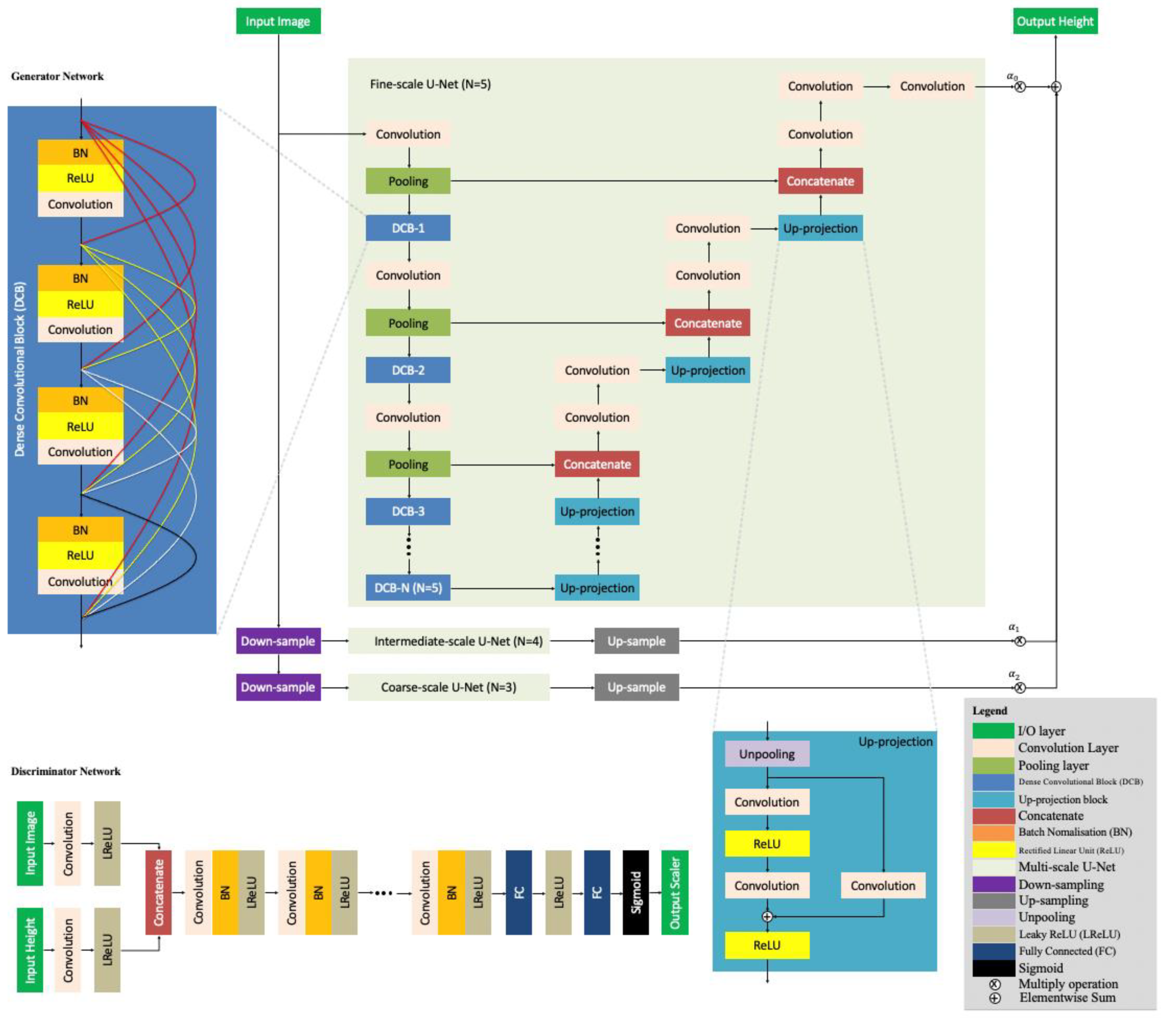
2.1. Network Architecture

GANs provide a state-of-the-art framework for generative tasks. In this work, we establish our MADNet model based on the GAN framework that we previously developed for super-resolution tasks [33]. For the generator, we replace the dense residual network in [33] with a U-Net based architecture [7] using DCB [8] for the encoder and up-projection [9] for the decoder. We adopt the adaptive weighted multi-scale reconstruction [33,34] concept for the generator network and the relativistic average discriminator [35] concept for the discriminator network.

Our proposed MADNet network architecture for single-image relative height estimation is shown in Figure 2. With MADNet, our goal is to train a generating function G that estimates a relative height map $H_{est}$, given a single input image I. Here $H_{est}$ is the estimated version of the “ground-truth” height map (also in relative values), i.e., $H_{gt}$, derived from stereo reconstruction methods using a higher resolution dataset. In order to achieve this, we train the multi-scale U-Net based generator network $G_{{\theta }_G}$ parameterised by ${\theta }_G$, where ${\theta }_G=\left\{W_{1:L};B_{1:L}\right\}$, W and B denotes the weights and biases of a L layer $G_{{\theta }_G}$, respectively. $\left\{W_{1:L};B_{1:L}\right\}$ is obtained by optimising the total loss function $l_{total}$ (see Section 2.2). For training images $I_{train}^n, n=1,2,\dots ,N$ and corresponding training height map $H_{gt}^n, n=1,2,\dots ,N$, our goal is to solve

$${\widehat{\theta }}_G=arg\underset{{\theta }_G}{\min }\frac{1}{N}{\displaystyle \sum }_{n=1}^N{l}_{total}(G_{{\theta }_G}(I_{train}^n),H_{gt}^n)$$

(1)

Following the GAN framework [6], the discriminator network $D_{{\theta }_D}$ parameterised by ${\theta }_D$ should be optimised in an alternating manner along with $G_{{\theta }_G}$ in order to solve the adversarial min-max problem of Equation (2), which is based on the general idea of training a generative model G with the goal to fool a discriminator D that is trained in parallel to distinguish estimated height map $H_{est}$ from ground-truth height map $H_{gt}$.

$$\underset{{\theta }_G}{\min } \underset{{\theta }_D}{\max } {\mathbb{E}}_{H_{gt}~H_{gt}^{1\to N}}\left[\log D_{{\theta }_D}(H_{gt})\right]+{\mathbb{E}}_{I_{train}~I_{train}^{1\to N}}[\log (1-D_{{\theta }_D}(G_{{\theta }_G}(I_{train})))]$$

(2)

The MADNet generator G consists of three adaptively weighted U-Nets at different scales, i.e., the fine-scale, the intermediate-scale, and the coarse-scale (see Figure 2). The fine-scale U-Net contains five convolution-pooling-DCB stacks to encode the input image I into a feature vector. The vector is then fed into five stacks of up-projection block, concatenation (with the corresponded output of each pooling layer of the encoder), and convolutional layers to reconstruct the height map $H_{est}^0$ at the fine-scale (level-0).

The intermediate-scale U-Net contains four convolution-pooling-DCB stacks to encode a downsampled version (two times lower resolution) of the input image, i.e., $f_{ds}(I)$, where $f_{ds}$ denotes the down-sampling operation, and contains four stacks of up-projection, concatenation, and convolutional layers to reconstruct the height map $H_{est}^1$ at the intermediate-scale (level-1). Finally, the coarse-scale U-Net contains three convolution-pooling-DCB stacks to encode a downsampled version (four times lower the resolution) of the input image $f_{ds}(f_{ds}(I))$, and 3 stacks of up-projection, concatenation, and convolutional layers to reconstruct the height map $H_{est}^2$ at the coarse-scale (level-2).

The weighted sum of $H_{est}^0$, $H_{est}^1$, and $H_{est}^2$ forms the final height map $H_{est}$.

$$H_{est}={\alpha }_0{H}_{est}^0+{\alpha }_1{f}_{up}(H_{est}^1)+{\alpha }_2{f}_{up}(f_{up}(H_{est}^2))$$

(3)

where $f_{up}$ denotes the up-sampling operation, ${\alpha }_0$, ${\alpha }_1$, and ${\alpha }_2$ are the adaptive weights of the three different scales, introduced to allow effective learning of both large-scale and small-scale height variations. The three U-Nets, $H_{est}^{5-N}$, where N denotes the depth of the multi-scale U-Net (N = 3, 4, 5), can be expressed as an encoding-decoding process as follows

$$H_{est}^{5-N}=f_{rec}(T_{dc}^N)=f_{rec}(f_{dc}^N(f_{ec}^N(I)))$$

(4)

where $f_{ec}^N$ denotes the encoding process, $f_{dc}^N$ denotes the decoding process, and $f_{rec}$ denotes the final reconstruction convolutional (3 × 3) layer that brings the decoded tensor, i.e., $T_{dc}^N$, to the same dimension as $H_{gt}$ ($H_{gt}$ and $H_{est}$ are at half the resolution of input image I in this work).

The encoding process in Equation (4) can be described as

$$T_{ec}^N=f_{ec}^N(I)=f_{DCB}^N(f_{pool}^N(f_{conv}^N(\dots f_{DCB}^1(f_{pool}^1(f_{conv}^1(I)))\dots )))$$

(5)

where $T_{ec}^N$ denotes the encoded tensor of the input image I, $f_{conv}$ denotes the convolutional operation, $f_{pool}$ denotes the pooling operation, and $f_{DCB}$ denotes the operation of DCB [8].

The encoding process, as shown in Equation (5), starts from a convolutional layer (7 × 7 kernel, 64 feature maps, stride 2) and a max-pooling layer (3 × 3 kernel, stride 2), followed by N DCBs, each of which are followed by convolutional layers (1 × 1 kernel, stride 1, and with increasing number of feature maps of 64, 128, 256, …) and average pooling layers (2 × 2 kernel, stride 2).

For DCB, we follow the original design as described in [8], wherein DCBs were proposed to connect multiple layers directly with each other to ensure maximum information flow between layers in the network. One of the issues of the increasingly deep CNNs is that the information contained in the input, or its gradient may get washed out before it reaches the end of the network when passing through many layers. In contrast to the dense residual blocks used in MARSGAN [33], DCB combines features by concatenating the feature maps from each previous layer instead of using summation. Having much fewer parameters to train is the most significant advantage of using DCB, especially when there is a limited training dataset. A $J$ layer DCB, i.e., $f_{DCB}$, has $\frac{J(J+1)}{2}$ connections since each of the j-th layer of a DCB has j inputs ($j\in J$) consisting of feature maps of all preceding convolutional blocks.

An $J$ layer DCB, can be formulated as a sequence of non-linear operations, denoted by $f_{nt}$, then the output of the j-th layer DCB, i.e., $x_{j+1}$, can be formulated as

$$x_{j+1}=f_{nt}(\left[x_0,x_1,\dots ,x_j\right])$$

(6)

where $f_{nt}$ can be defined as a sequential operation of Batch Normalisation (BN), Rectified Linear Unit (ReLU) function, and convolution.

The decoding process in Equation (4) can be expressed as

$$T_{dc}^N=f_{dc}^N(T_{ec}^N)=f_{conv}^N(f_{conv}^N(P^1\parallel f_{UPB}^N(\dots f_{conv}^1(f_{conv}^1(P^N\parallel f_{UPB}^1(T_{ec}^N)))\dots )))$$

(7)

where $f_{UPB}$ denotes the operation of up-projection [9], and P denotes the output of the pooling layers of the encoder, which is concatenated with the corresponding output of the up-projection block in a reversed order, e.g., $P^5\parallel$ $f_{UPB}^1(*)$, $P^4\parallel$ $f_{UPB}^2(*)$, …, $P^1\parallel$ $f_{UPB}^5(*)$ for the fine-scale U-Net (N = 5).

The encoding process, as shown in Equation (7), consists of N up-projection operations (N $f_{UPB}$), each of which are followed by concatenation and two convolutional layers (3 × 3 kernel, stride 1, and with decreasing number of feature maps, which are in an inverted order of the convolutional layers of the encoder).

Each of the up-projection blocks, following the original design described in [9], consists of an unpooling layer, two branches of convolutional layers to connect the lower resolution feature map with the up-sampled feature map. In particular, unpooling is the inverse operation of the pooling layer, as used in the encoder, designed to restore (increase) the spatial size of the feature maps. Unpooling layer maps each input entry into the top-left corner of a 2 × 2 kernel (fill 0s for the rest), which is then followed by the convolutional layers to remove the 0 s, to achieve “up-convolution”.

For the discriminator, we slightly modify the architecture that was used in [33] to include a concatenation layer that concatenates the input image I with the height-map H. The discriminator network consists of 8 convolutional layers with an increasing number of feature maps and strides of 2 each time the number of features is doubled (3 × 3 kernels; 64 feature maps, stride 1; 64 feature maps, stride 2; 128 feature maps, stride 1; 128 feature maps, stride 2; …; 512 feature maps, stride 1, 512 feature maps, stride 2). The resulting 512 feature maps are followed by two fully connected dense layers together with a final sigmoid activation function to output a single scalar. The scalar represents the probability that the input is relatively more likely from $H_{gt}$ than all $H_{est}$ on average (within a mini-batch), or relatively less likely from $H_{gt}$ than all $H_{gt}$ on average (within a mini-batch). This concept was proposed in [35], namely, the relativistic average discriminator.

Let $D_{Ra}$ denote the relativistic average discriminator, for real input $H_r$ and fake input $H_f$, $D_{Ra}$ can be expressed as

$$\{\begin{array}{c}{D}_{Ra}(H_r,H_f)=\sigma (C(H_r)-{\mathbb{E}}_{H_f}(C(H_f)))\to 1(more real than fake)\\ D_{Ra}(H_f,H_r)=\sigma (C(H_f)-{\mathbb{E}}_{H_r}(C(H_r)))\to 0(less real than real)\end{array}$$

(8)

where $\sigma$ is the sigmoid function, C is the non-transformed discriminator output, and ${\mathbb{E}}_{H_f}$ and ${\mathbb{E}}_{H_r}$ represent the operation of computing the mean of all fake inputs and all real inputs in a mini-batch, respectively.

2.2. Loss Functions

The standard loss function for optimisation of the regression problem is the $l_2$ loss, minimising the squared Euclidean norm between the generated predictions and ground-truth. In the field of monocular depth estimation, many different loss functions have been proposed. These include the early work from [15] who used scale-invariant loss (mean squared error of the depth in log space), which has been improved in [16] as the local structure loss (the gradients of the depth difference in the horizontal and vertical directions). It is worth noting that the Structure Similarity Index Measurement (SSIM) [36] based loss has also been widely used in monocular depth estimation tasks, but SSIM loss is mostly used in unsupervised cases to quantify the differences between back-projected images. This is demonstrated in [37] who coupled the SSIM loss with $l_1$ loss. Finally, the Berhu [38] loss was also proven optimal to $l_2$ based loss functions in [9]. In this work, we use a weighted sum of the gradient loss (denoted as $l_{grad}$), the Berhu loss (denoted as $l_{bh}$), and the adversarial loss under the GAN framework (denoted as $l_{gen}$) as our total loss function to solve Equation (1). This can be expressed as

$$l_{total}=\lambda l_{grad}+\gamma l_{bh}+\eta l_{gen}$$

(9)

where $\lambda$, $\gamma$, and $\eta$ are the hyperparameters to balance different loss terms.

The gradient loss of Equation (9) can be expressed as

$$l_{grad}=\frac{1}{RC}{\displaystyle \sum }_{r=1}^R{\displaystyle \sum }_{c=1}^C[{({\nabla }_x(H_{gt},H_{est}))}^2+{\nabla }_y{(H_{gt},H_{est})}^2]$$

(10)

where r and c are the row and column of a R-row and C-column height map H, respectively ${\nabla }_x$ and ${\nabla }_y$ compute the differences of the horizontal and vertical gradients of the height maps, respectively.

The Berhu loss of Equation (9) can be expressed as

$$l_{bh}(H_{gt},H_{est})=\{\begin{array}{c}\left|H_{gt}-H_{est}\right|, if \left|H_{gt}-H_{est}\right|\le \tau \\ \frac{{(H_{gt}-H_{est})}^2+{\tau }^2}{2\tau }, if \left|H_{gt}-H_{est}\right|>\tau \end{array}$$

(11)

where $\tau$ is a threshold that is set to $\tau =\frac{1}{5}{\max }_{r,c}(\left|H_{gt}-H_{est}\right|)$, so when $\left|H_{gt}-H_{est}\right|\le \tau$, $l_{bh}(H_{gt},H_{est})$ equals to the $l_1$ loss, and when $\left|H_{gt}-H_{est}\right|>\tau$, $l_{bh}(H_{gt},H_{est})$ equals to the $l_2$ loss.

Finally, based on Equations (2) and (8), the relativistic discriminator loss [35], denoted as $l_d$ can be expressed as

$$l_d=-{\mathbb{E}}_{H_r}\left[\log (D_{Ra}(H_r,H_f))\right]-{\mathbb{E}}_{H_f}\left[\log (1-D_{Ra}(H_f,H_r))\right]$$

(12)

The adversarial loss in Equation (9) can be expressed as a symmetrical form of Equation (12)

$$l_{gen}=-{\mathbb{E}}_{H_r}\left[\log (1-D_{Ra}(H_r,H_f))\right]-{\mathbb{E}}_{H_f}\left[\log (D_{Ra}(H_f,H_r))\right]$$

(13)

Training of the MADNet follows the stochastic gradient descent approach of the relativistic average GAN framework [35]. Based on Equations (2) and (8), initially, ${\theta }_D$ is updated by ascending the stochastic gradient of

$${\nabla }_{{\theta }_D}{\mathbb{E}}_{\mathrm{m}~\mathrm{M}}\left[{\mathbb{E}}_{H_f}(C_{{\theta }_D}(G_{{\theta }_G}(I_{train})))-C_{{\theta }_D}(H_r)+C_{{\theta }_D}(G_{{\theta }_G}(I_{train}))-{\mathbb{E}}_{H_r}(C_{{\theta }_D}(H_r))\right]$$

(14)

for samples m in a mini-batch M, and $I_{train},H_f,H_r\in M$. Then update ${\theta }_G$ by ascending the stochastic gradient of

$${\nabla }_{{\theta }_G}{\mathbb{E}}_{\mathrm{m}~\mathrm{M}}\left[{\mathbb{E}}_{H_r}(C_{{\theta }_D}(H_r))-C_{{\theta }_D}(G_{{\theta }_G}(I_{train}))+C_{{\theta }_D}(H_r)-{\mathbb{E}}_{H_f}(C_{{\theta }_D}(G_{{\theta }_G}(I_{train})))\right]$$

(15)

then iteratively update ${\theta }_D$ and ${\theta }_G$ in the next mini-batch (iteration) until all training iterations complete.

The loss function plays an important role in deep learning methods. In this work, we use a combination of three commonly used loss functions, including the standard adversarial loss as under the generative adversarial framework, the standard Berhu loss that directly measures the difference between the prediction and the ground-truth height map, and the gradient loss to penalise the structural similarity of the prediction and the ground-truth height map. This is a basic and practical combination of a variety of loss functions that have been proposed in the field of monocular depth estimation. Although it performs well for this work after some tuning of the weights (provided in Section 2.4), there is still room to improve in the future with more experiments. For example, we have not yet found an efficient way of penalising the high-frequency depth details.

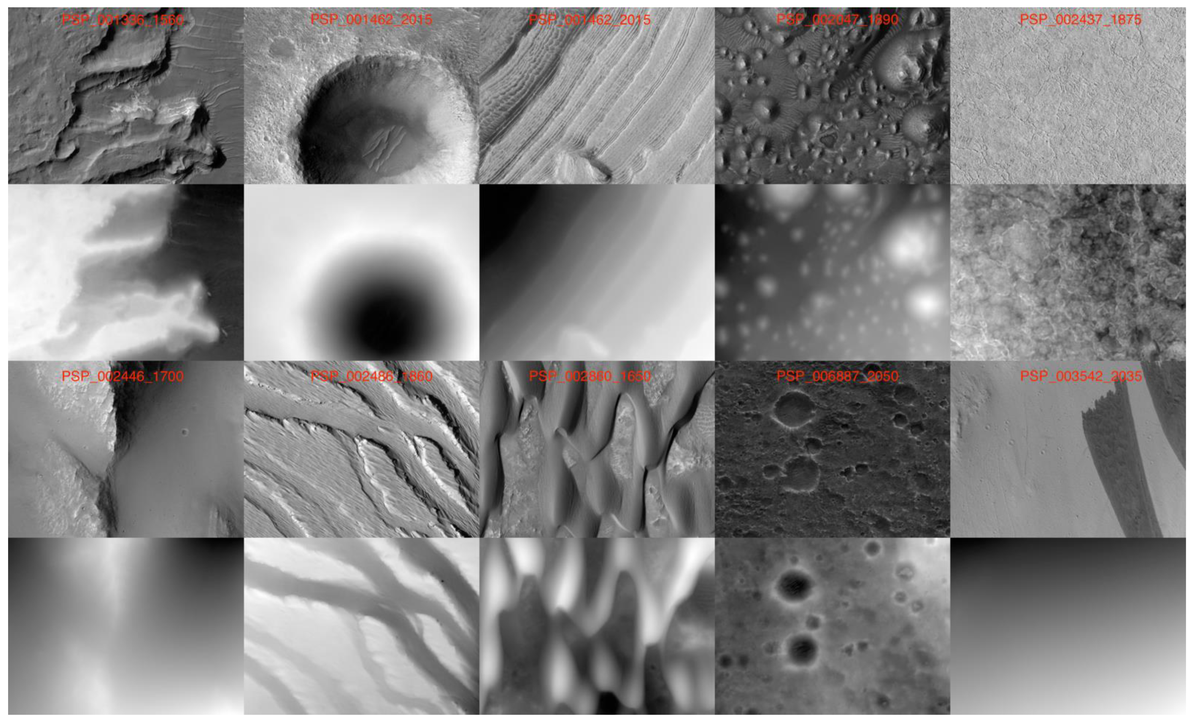
2.3. Training Dataset

Our training datasets are formed from 450 unique HiRISE PDS ORIs (0.25 cm/pixel) and DTMs (1 m/pixel) that are available through the University of Arizona’s HiRISE site (see https://www.uahirise.org/dtm/ (accessed on 21 July 2021)). These ORI/DTM products are manually selected to contain a variety of different features of the Martian surface with fairly good quality.

We form two sets of training datasets, for network initialisation and for full training. The first training dataset contains 4,200 (12,600 after data augmentation) pairs of cropped and randomly selected samples (512 × 512 pixels) of the ORIs and DTMs at lower spatial resolution (4 m/pixel) and is used for initial training of the network. Down-sampling of the original HiRISE ORIs and DTMs is achieved using the GDAL’s “cubicspline” resampling method (https://gdal.org/programs/gdal_translate.html (accessed on 21 July 2021)). For each DTM cropped sample, the height values are rescaled to relative floating-points values in the range of [0, 1] from their original min/max height values. Note that we do not normalise the digital values of the ORIs in this work. During the HiRISE cropping process, if any of the ORI or corresponding DTM crop contains “nodata” value, then the paired ORI and DTM samples are removed from the training dataset. The second training dataset contains 15,500 (46,500 after data augmentation) pairs of cropped samples (512 × 512 pixels) of the ORIs and DTMs downsampled at 2 m/pixel and is used for full training of the network. Some examples of the second training dataset are shown in Figure 3 (HiRISE image IDs are shown on each sub-figures). This collection of examples contains a variety of different surface features, such as large-structures, large-sized craters, layers on slopes, cones, small-scale semi-flat features, high-peaks, layered peaks, dunes, small-sized craters, and flat features on slopes (in the order of top-left-to-bottom-right).

For both of the two training datasets, we manually scan all DTM crops, and removed the paired samples, when artefacts or significant noise are found. The artefact/noise could be minor errors in a full-strip DTM, but they become obvious after rescaled (stretched) within a small crop. The aforementioned numbers of the two training datasets are after these scenes were removed. For training data augmentation, we apply both vertical and horizontal flipping. Such data augmentation processes enrich our training datasets, can help prevent overfitting in training, and meanwhile reduce the effect of the similar shading directions from HiRISE as captured in similar Mars local time.

It should be noted that we do not use the original resolution of the PDS DTMs in this work, because the effective resolution of the HiRISE DTMs is generally lower than 1 m/pixel, as we can observe that there are fewer details from the PDS DTM in comparison to the 1 m/pixel downsampled ORI. We deem the spatial resolution of the DTMs are approximately between 2 m/pixel and 4 m/pixel. In order to achieve semi-pixel-to-pixel level image-to-height learning, the full training is achieved at a scale of 2 m/pixel.

2.4. Training Details

We propose a two-stage training for the proposed MADNet. At the first stage, initial training is achieved on each of the three single-scale adversarial U-Nets, with the lower-resolution training dataset. Note the U-Net encoders are pre-initialised using ImageNet [39]. The first stage training has 78,750 iterations, with a batch size of 8, and with an initial learning rate of ${10}^{-4}$ with standard Adam optimisation [40] (${\beta }_1=0.9$ and ${\beta }_2=0.999$). The weights of the loss function in Equation (9) are set at $\lambda =0.5$, $\gamma =5\times {10}^{-2}$, and $\eta =5\times {10}^{-3}$. For the second stage, the multi-scale adversarial U-Nets are trained jointly, with each of them pre-trained for the first stage and initialised with adaptive weights of ${\alpha }_0=0.5$, ${\alpha }_1=0.25$, and ${\alpha }_2=0.25$ as shown in Equation (3). The second stage training achieved 581,250 iterations, with a batch size of 8, and the learning rate and loss function setups as the first stage training. All training and testing are achieved on the latest Nvidia^® RTX3090^® GPU.

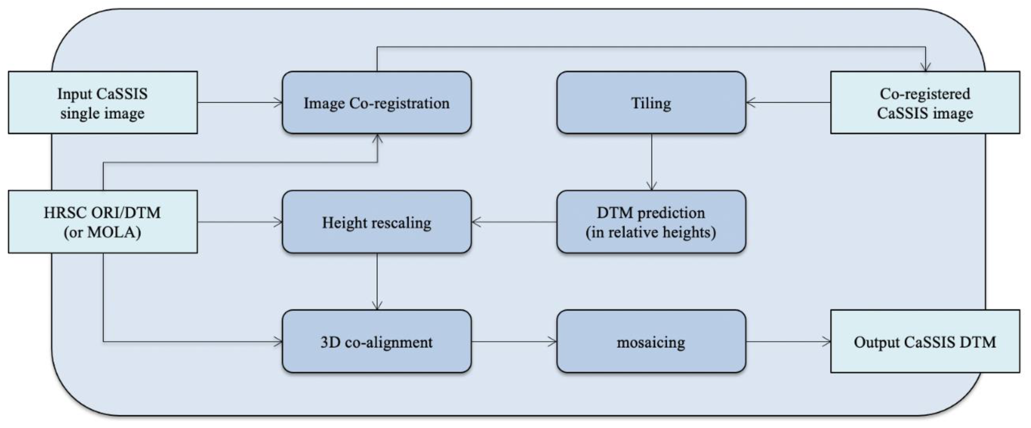
2.5. Overall Processing Chain

The MADNet single-image height prediction process still has several restrictions. In this section, we resolve these remaining issues with pre-processing and post-processing methods. Firstly, the input image size for MADNet is limited to 512 × 512 pixels subject to the design of the network and GPU memory constraints. In order to achieve full-strip DTM prediction, we need to use tiling and mosaicing processes at the pre-processing and post-processing. Secondly, the predicted heights are in relative height units with a scale of [0, 1] the same as the rescaled training datasets. In order to recover the absolute heights, we use reference HRSC DTM (for this work) or MOLA DTM (in general) to rescale the relative heights. Thirdly, the geo-information encoded within the CaSSIS images currently has a systematic error, due to issues with the onboard clock. In this case, we cannot directly use a MOLA DTM for rescaling as the spatial locations of CaSSIS are wrong. Therefore, we include image co-registration of CaSSIS and HRSC in a pre-processing in order to achieve the height rescaling using HRSC DTM.

An overall processing chain for the proposed MADNet based single-image CaSSIS DTM processing system is shown in Figure 4. This includes six steps and can be briefly summarised as follows: (1) CaSSIS-to-HRSC image co-registration, following our in-house feature matching and fitting algorithms described in [41,42]; (2) cropping of the co-registered CaSSIS image into small overlapping tiles (512 × 512 pixels per tile, with 100–150 overlapping pixels in the horizontal and vertical directions) and simultaneously storage of the geo-headers of each of the tiles that need to be re-attached to the output DTM tiles (geoinformation is not kept within the prediction process); (3) batch MADNet prediction of all input tiles; (4) re-attach the geo-header files of the input image tiles from step (2) to the output DTM tiles from step (3), and rescale the height range of the DTM tiles from [0, 1] to [min, max] using the corresponding HRSC DTM; (5) 3D co-alignment of the rescaled DTM tiles using a reference DTM, which could be MOLA, HRSC (as used in this work), CTX stereo products, or the United States Geological Survey (USGS) MOLA-HRSC blended DTM product (available at https://astrogeology.usgs.gov/search/map/Mars/Topography/HRSC_MOLA_Blend/Mars_HRSC_MOLA_BlendDEM_Global_200mp (accessed on 21 July 2021)); (6) finally we achieve DTM blending and mosaicing with the Ames Stereo Pipeline [43] “dem_mosaic” function (see https://github.com/NeoGeographyToolkit/StereoPipeline (accessed on 21 July 2021)).

2.6. Study Sites

The main experiments shown here are made over the Rosalind Franklin ExoMars 2022 rover’s landing site at Oxia Planum [11]. Oxia Planum (centred near 18.275°N, 335.368°E) is on the south-eastern edge of Chryse Planitia, one of the three main basins that comprise the northern plains of Mars. The landing site is at around 18°N and located at the mouth of several channels that drain from the southern uplands. One of the drivers for selecting this site was that the area is characterised by extensive clay minerals, thought to present excellent targets for seeking potential biomarkers–one of the primary objectives of the mission.

We use two other sites to demonstrate the potential of MADNet. The first is a landslide in the southern part of Baetis Chaos. The chaos terrain forms a depression that is thought to have been formed by collapse engendered by the outflow from an underground aquifer (e.g., [44]). On the southern wall of the depression, there are a series of landslides, which overlie the ejecta deposits of a nearby fresh 13 km diameter complex impact crater. Because of this superposition, we know that the impact did not directly cause the landslides, but it may have weakened the bedrock in the area leading to their formation.

The second site is located in Aeolis Mensae, an area characterised by wind erosion of a thick pile of sedimentary rocks (e.g., [45]). The region is crossed by the Aeolis Dorsa, thought to represent inverted channel deposits (e.g., [46]). In this particular scene, there are numerous yardangs and two notable ridges, which are likely inverted channels, running broadly east-west, which join a fan shaped-deposit with distributary-ridges to the east [47].

3. Results

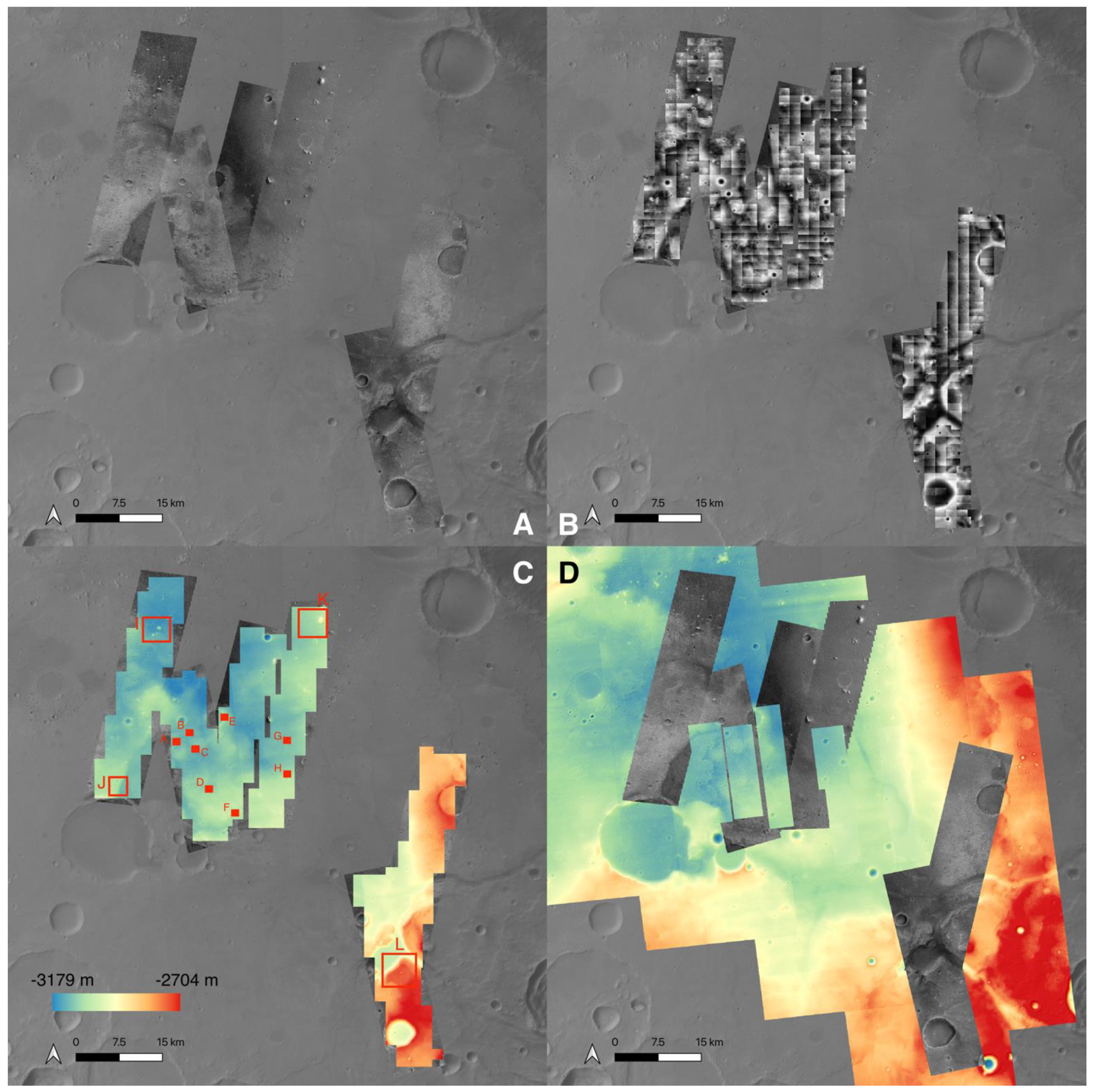
3.1. Overview of Data and Products for Oxia Planum

Our test inputs for Oxia Planum include six 4 m/pixel CaSSIS panchromatic band images (the image IDs are MY34_003806_019_1; MY34_005664_163_1; MY35_006504_018_0; MY35_007337_020_0; MY35_007623_019_0; MY35_008275_165_0). Our reference dataset is the 12.5 m/pixel MC11-West ORI mosaic and 50 m/pixel MC11-West DTM mosaic produced by the HRSC team (HMC_11W24_nd5 and HMC_11W20_da5; available at http://hrscteam.dlr.de/HMC30 (accessed on 21 July 2021)). We use the 20 m/pixel CTX DTM Oxia Planum mosaic produced by the Natural History Museum (London) and Open University (CTX_OXIA_DTM_20m_r) and the 1 m/pixel HiRISE PDS DTMs (the image IDs are DTEEC_009880_1985_009735_1985_L01; DTEEC_036925_1985_037558_1985_L01; DTEEC_003195_1985_002694_1985_L01; DTEEC_039299_1985_047501_1985_L01; DTEEC_042134_1985_053962_1985_L01; available through the University of Arizona’s HiRISE site at https://www.uahirise.org/dtm/ (accessed on 21 July 2021)) as our validation datasets.

Figure 5 shows an overview of the aforementioned datasets, and our results from the proposed MADNet single-image CaSSIS DTM processing system, over the Oxia Planum area. Figure 5A shows the 6 input CaSSIS panchromatic band images (after co-registration) superimposed on the HRSC MC11-West ORI mosaic. Figure 5B shows the tiled CaSSIS DTM predictions (in relative height values of [0, 1]), which are the outputs from step (4) of the overall processing chain described in Section 2.5, superimposed on the 6 CaSSIS images and HRSC. Figure 5C shows the final mosaiced CaSSIS DTM at 8 m/pixel using the proposed MADNet method (after height rescaling from relative [0, 1] to absolute [min, max] of the HRSC MC11-West DTM mosaic over the same location. The mosaiced CaSSIS DTM shows no transition error/artefact between adjacent tiles. Figure 5D shows the 6 available HiRISE PDS DTMs (for validation) superimposed on the 6 CaSSIS image, CTX DTM mosaic, and HRSC MC11-West ORI mosaic. It should be noted that in order to achieve a more accurate comparison, in Section 3.2, we co-align our CaSSIS DTM results and the HiRISE PDS DTM with the CTX DTM mosaic, which is pre-aligned with the HRSC MC11-W ORI/DTM and MOLA.

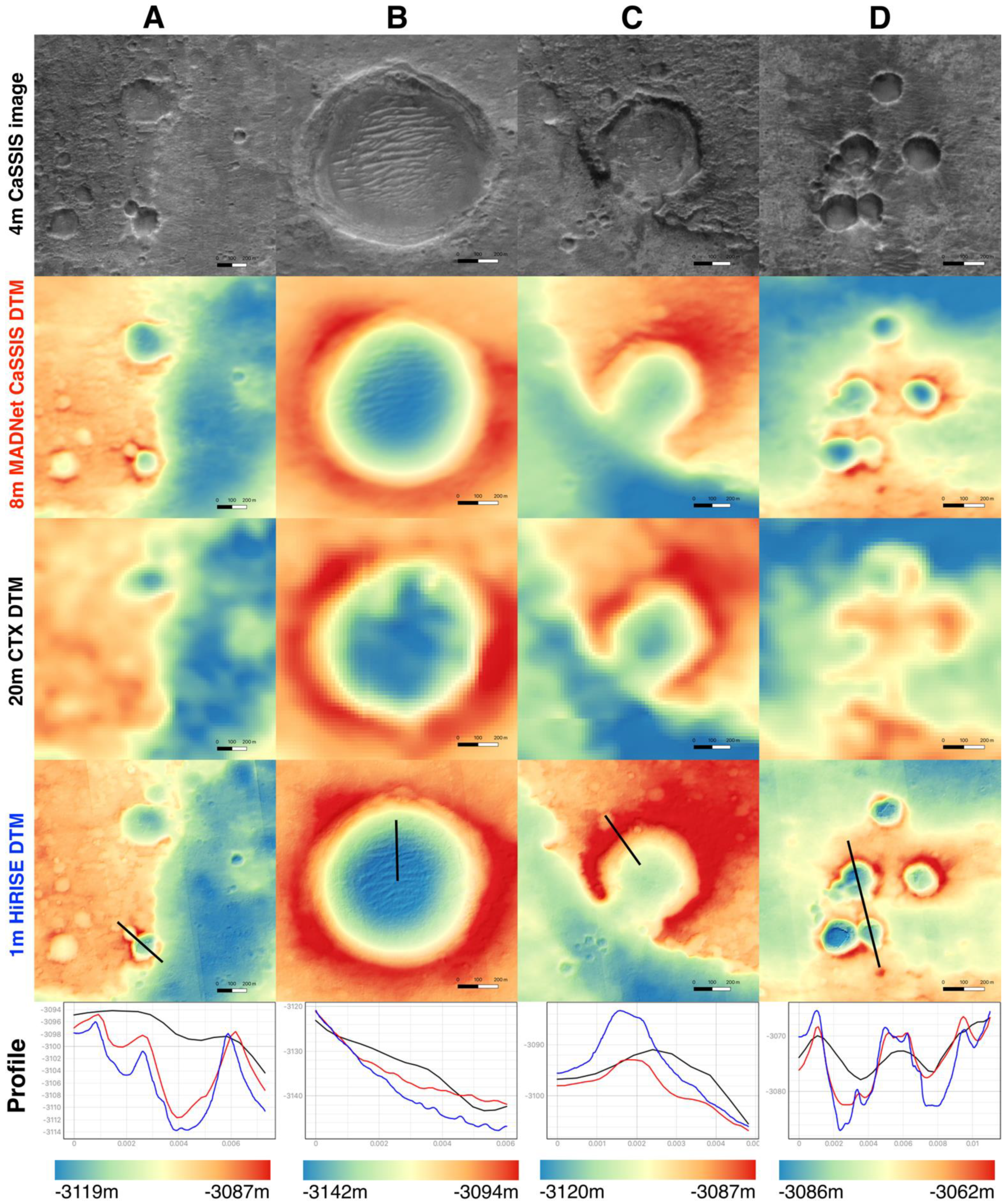
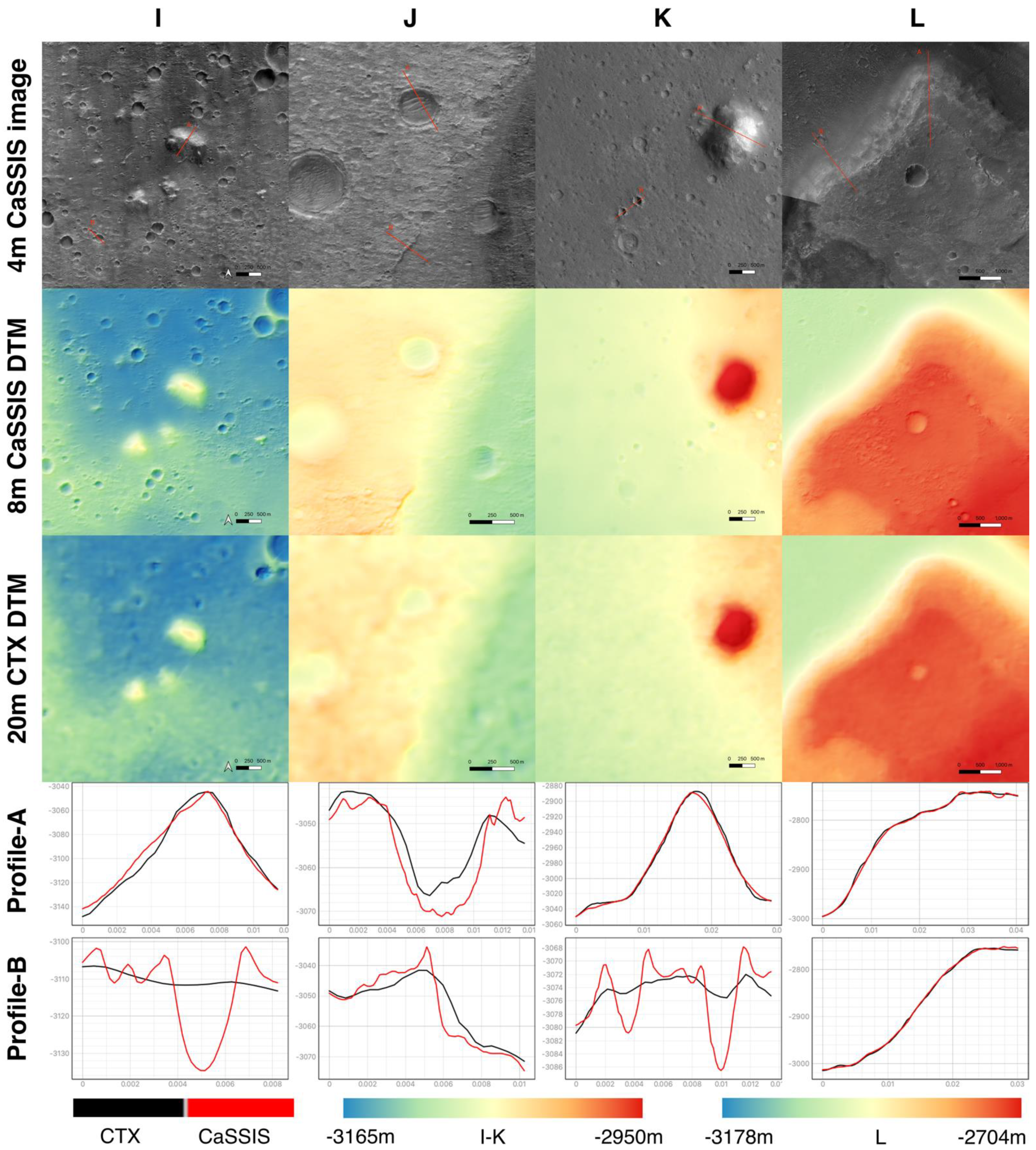
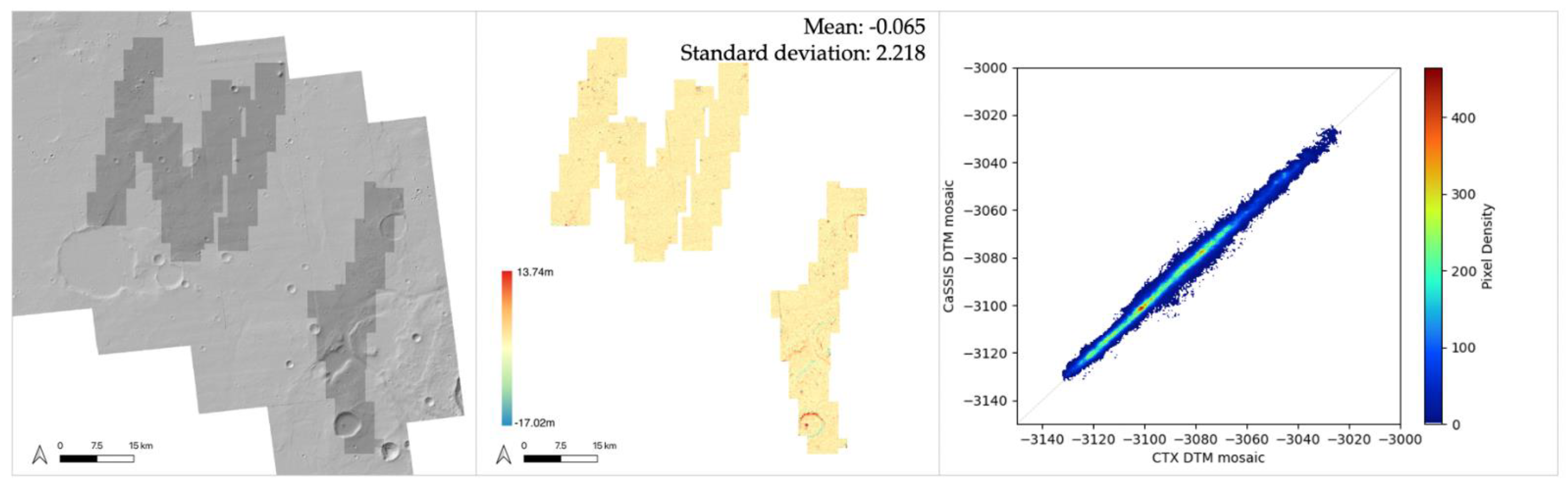
3.2. Oxia Planum Results and Assessments

In this section, we compare in small-scale details of the resultant 8 m/pixel CaSSIS DTM, validation 20 m/pixel CTX DTM, and validation 1 m/pixel HiRISE DTM, for 8 selected areas (A–H) that have overlapping HiRISE PDS DTM available. We further compare in larger-scale of the resultant 8 m/pixel CaSSIS DTM and validation 20 m/pixel CTX DTM, for four selected areas (I–L) that do not have overlapping HiRISE PDS DTM available. We tend to select areas that contain more terrain variations (like craters or peaks) in order to better assess the results. Locations of all areas (A–L) are shown and labelled in Figure 5C.

Figure 6 shows zoom-in views of the 4 m/pixel CaSSIS image, 8 m/pixel MADNet CaSSIS DTM, 20 m/pixel CTX DTM, 1 m/pixel HiRISE DTM, and measured profiles (location shown on the HiRISE DTMs), for areas A, B, C, and D. In general, we observe good alignments for CaSSIS, CTX and HiRISE DTMs. The maximum measured difference for all three DTMs are within 12 m. CaSSIS DTM tends to have better agreement with CTX DTM in all places, and meanwhile shows the small topographic details that have fairly good agreement with the corresponding HiRISE DTM. No obvious artefact is found from the MADNet CaSSIS DTM in all areas. Noting the small craters in areas A and D, and rippled dune feature in area B, have both been successfully captured and reconstructed by MADNet. The CaSSIS DTM shows a lower crater edge in area C compared to the HiRISE DTM, however, the CaSSIS DTM shows less overshoot and undershoot of the crater edges in area D.

Figure 7 shows zoom-in views of the 4 m/pixel CaSSIS image, 8 m/pixel MADNet CaSSIS DTM, 20 m/pixel CTX DTM, 1 m/pixel HiRISE DTM, and measured profiles (location shown on the HiRISE DTMs), for areas E, F, G, and H. In general, the same characteristics from Figure 6 can also be observed in these 4 areas, good agreement between CaSSIS DTM and CTX DTM at the large-scale, while at small-scale, CaSSIS DTM is picking up a similar level of details as HiRISE DTM. Noting in area E, the two connected peaks seem to have different heights, whereas the CaSSIS DTM is opposite to the HiRISE DTM. Looking on the image, the CaSSIS DTM seems to be visually more correct. Area F and G also shows good agreement at the crater edges for all 3 DTMs. It is worth pointing out, in area H, there is a very small peak at the centre of the crater. This information has been successfully picked up with MADNet. The relative height for the small peak in the CaSSIS DTM is very similar to the HiRISE DTM, despite the CaSSIS DTM being better correlated to the CTX DTM at a larger scale.

In Figure 8, we show 4 further areas, i.e., I, J, K, and L, where there are no HiRISE stereo data. Zoom-in views and profile measurements (location shown on the CaSSIS images) are given for 8 m/pixel MADNet CaSSIS DTM and 20 m/pixel CTX DTM. We can observe good alignment between the CaSSIS DTM and CTX DTM in general, while the CaSSIS DTM shows more details. In particular, area I is a field with many small and medium sized craters, and the MADNet results have obviously captured more craters and there is no generative artefact found for the craters. Area I also shows good agreement in height between the CTX DTM and CaSSIS DTM for a small hill in the centre. Area J shows MADNet has successfully captured the rippled dunes inside the crater as well as a sharp peak feature in the south. Areas K and L also show good alignment between the CTX and CaSSIS DTMs, and meanwhile shows more details in the CaSSIS DTM.

We observe no artefacts from the DTM results using the proposed MADNet system with the 6 CaSSIS images. The CaSSIS DTM effective resolution (although sampled at 8 m/pixel) appears qualitatively to be very similar to the 1 m/pixel HiRISE DTM. For areas with or without available HiRISE DTM, the CaSSIS DTM mosaic shows consistently good agreement with the 20 m/pixel CTX DTM mosaic, while capturing more details, like craters and small peaks. The hill-shaded images, difference map, and scatter plot for the CaSSIS and CTX DTM mosaics are shown in Figure 9. We can observe a good correlation between the CaSSIS and CTX DTM mosaics.

In addition to the visual comparisons of the DTMs and their associated profile analysis, hill-shaded images using eight different azimuth angles at 45° increments from 0° to 315°, and 30° of illumination elevation, for eight randomly selected peak and crater areas are shown in Figure 10. No artefacts are found in these results.

3.3. Science Case Study: Site-1

Figure 11 shows that metres to tens of metres details of the landslide and its surrounding terrain have been successfully captured by MADNet. Of particular interest is the fact that the topographic signature of the bedrock spurs located near the top of the escarpment are clearly visible. The topography of these spurs can give important information on erosion rates of the bedrock (e.g., [48]). In addition, the subtle topography related to the parallel ridges and troughs running northwest-to-southeast which represent the underlying crater ejecta, are also partially reproduced and their topographic relief can be used to better understand the surface over which the landslide propagated. Finally, the lateral levees, toe scarp, and detailed surface textures of the landslide deposits are reproduced (including superposed small craters), which is of use for understanding the dynamics of the landslide (e.g., [49]). On the other side, the CaSSIS DTM has not shown so well at the hundred-metre to kilometre-scale where some details have been smoothed out, including some of the bulges on the deposit and the fallen block of the plateau. This is mostly due to the final 3D co-alignment process using a coarse reference DTM that cancelled some of the large-scale topography or falsely correctly the MADNet DTM onto a reference that has large-scale artefacts. Please refer to Section 4.3 for discussions on this. This can be improved in the future using a coarse-to-fine approach (i.e., to produce MADNet HRSC DTM at higher resolution using MOLA as the reference, then produce MADNet CaSSIS DTM using the MADNet HRSC DTM as the reference).

3.4. Science Case Study: Site-2

Figure 12 shows that MADNet has successfully reproduced the metre to tens of metre scale topographic features in the Aeolis Mensae region, including north-south elongated yardangs and subtlety expressed eroded impact craters. In the south part of Figure 12 layers in the eroded bedrock are picked out in topographic relief and are only metres in thickness. Topographic analysis of sedimentary deposits is important for understanding their rate of formation and erosion (e.g., [50]). On the other side, the flat-topped nature of the ridge and its overall elevation changes along its length do not seem to have been kept in the final resultant DTM, but instead to be over-influenced by the HRSC topography during 3D co-alignment. To correct this, a coarse-to-fine step (MOLA-MADNet HRSC-MADNet CaSSIS) can be followed.

4. Discussion

4.1. Photogrammetry, Photoclinometry, or Deep Learning?

In this section, we briefly discuss the pros and cons of the three different types of DTM production approaches for Mars orbital data. We believe this discussion would provide the readers with some perspective and outlook to introducing more deep-learning-based approaches into planetary mapping in the near future. We compare the three approaches in five aspects, i.e., artefactual, resolution, accuracy, flexibility, and speed.

The artefacts in photogrammetry generally have the appearance of obvious error, such as stripes, gaps, patterned noise, or discrete fluctuation. In general, artefacts from photogrammetry methods are fairly common, especially when input images are different in imaging conditions (e.g., contrast, shading, resolution, noise), and subsequently, additional efforts on post-processing are always required to reduce their effects. In particular, photoclinometry methods are sometimes employed to correct such photogrammetric artefacts [51]. However, new artefacts may be introduced from the photoclinometry method itself. These generally refer to overshooting, undershooting, or offsets. Due to the thin Martian atmosphere and limited availability of the atmospheric parameters and surface bidirectional reflectance distribution function (BRDF), photoclinometry for Mars is still challenging.

In contrast, a well-trained deep learning network has a much lower frequency to produce an artefact. However, any artefacts produced from a well-trained deep network could be very difficult to be detected, as they are unlikely to look like artefacts, and thus are more dangerous (like dark sand might be translated into lumps if the network not being able to see such features in training data). On the other hand, potential artefacts from photoclinometry and deep learning cannot be pre-modelled, whereas artefacts from photogrammetry can be automatically modelled or pre-detected via matching uncertainties [52]. For large-area mapping tasks, artefacts are almost inevitable with all methods, however, applying constraints using a reference source (like MOLA) could always limit the upper bounds of such artefacts.

In terms of resultant DTM resolution, photoclinometry generally produces per-pixel height reconstructions, thus has the highest resolution. Photogrammetry generally produces the lowest resolution among the three approaches as “averaging” is consistently introduced over the whole workflow through the application of area-based image matching procedures. A deep learning-based method should produce resolutions similar to photoclinometry but depends on whether there is sufficient training data. Even though the proposed supervised method is trained with photogrammetric DTMs, we can down-sample such DTMs (and associated ORIs) to their effective resolution and perform pixel-level image-to-height training/learning. In this way, artefacts could be mostly eliminated as they mostly occur in fine-scale features (in the case of the HiRISE PDS DTMs). N.B. Training DTMs that have large-scale errors or strong noise have been pre-removed as stated in Section 2.3. This also explains how deep learning-based methods are not reproducing any artefact that might be contained in the original training data. For example, after training with the down-sampled data, the network has learnt how to produce the best DTM for an “artefact-free” big crater, then the learnt parameter sets can be used to produce the most appropriate DTM for a much smaller crater, where many artefacts may appear using photogrammetry.

Not taking any potential artefacts into consideration or resolution differences, photogrammetry should have the highest (or most reliable) accuracy as the height values are based on solid computation without assumption/stochastic inputs. However, as a large proportion of the scene is likely to be affected more or less by matching artefacts/or post-smoothing (frequently used to reduce such artefacts) on real-world applications, due to various inferences and imperfections, and thus the above statement is only true “in theory”. Photoclinometry methods could be highly accurate for the Moon, but on Mars, it is considered less accurate due to issues with atmospheric dust scattering and unknown BRDF effects. According to [53], there are height variations of about 10–20 m, between the CaSSIS DTMs and HiRISE DTMs, that are commonly seen at crater ridges (known as “overshooting”), but in this work, such height variations at the same and other crater ridges are generally less than 5 m (10 m maximum) according to the profile measurements presented in Section 3.2.

In terms of flexibility and processing speed, the proposed MADNet system clearly outperforms photogrammetry and photoclinometry approaches by a large margin. Once the MADNet model is fully trained, which takes a few days on a Nvidia^® RTX3090 GPU, the DTM inference process only takes from a few seconds (e.g., CaSSIS and CTX) to a few minutes (e.g., HiRISE) without the need to know the camera models (as required by photogrammetry) or imaging, atmospheric and surface BRDF conditions (as required by photoclinometry). Adding in the required processing time from 3D co-alignments and other pre- and post-processing steps, producing a DTM from CTX and CaSSIS sized images generally takes ~20 min, and producing a DTM using MADNet from larger images like HiRISE generally takes 1–2 h. In contrast to photogrammetry approaches, based on our experience, producing a DTM from CTX and CaSSIS sized images generally takes about 3–10 h depending on the different stereo matching algorithms, and is also subject to trade-offs between the complexity of the processing system and the DTM quality. Producing a DTM from much larger images like HiRISE using photogrammetry often takes more than 8 h up to a few days. Photoclinometry, to the best of our knowledge, takes a similar or longer time to process than photogrammetry.

4.2. Extendibility with Other Datasets

This paper focuses on single-image fast DTM estimation of the TGO CaSSIS images. However, it should be pointed out that the proposed MADNet model can also be applied to other Mars datasets at different resolutions, e.g., HRSC, CTX, and HiRISE, without the need for re-training or parameter tuning. Figure 13 demonstrates the MADNet DTM results for HRSC, CTX, and HiRISE, which are produced instantly (in a few seconds for CTX and HRSC and less than a minute for HiRISE), in comparison to the photogrammetric DTM results from PSA (for HRSC) and PDS (for HiRISE). This experiment shows the proposed MADNet system outperforms photogrammetric methods both on speed and on quality.

4.3. Future Improvements

There is still room to improve the proposed method in many aspects, such as (1) re-defining the loss functions to take perceptual similarity into consideration; (2) re-designing the multi-scale scheme to deal with different performance on flat regions and steep slopes; (3) re-forming a better (larger) training dataset combining with different instruments; (4) using segmentation to help capture smaller features; (5) combining with shape-from-shading oriented networks [54] using a multi-stage reconstruction strategy.

In particular to point (2), we observed the fact that MADNet (with the current available training dataset) has poorer performance for capturing fine-scale details on steep slopes and on comparably flatter terrain. See Figure 14 as an example (see arrowed areas on the CaSSIS image and measured height profile) demonstrating the height variations on steep slope appears to be too small (smooth). Note that there is no HiRISE or CTX stereo data available for this area. This could be an issue with the current multi-scale implementation that when coarse-scale height variation dominates an input tile, fine-scale variation is neglected in the intermediate-scale U-Net and thus not receiving enough attention in the network. Future improvement could be implemented to use the height variation of the coarse-scale prediction as a threshold to control the reconstruction strategy of the two finer-scale predictions. Point (4) may also be a way forward to improve this issue.

As for discussion point (3), currently, the finest scale U-Net is trained with 2 m/pixel HiRISE ORI/DTM samples and the two coarser scale U-Nets are trained with 4 m/pixel sample. However, if there are more high-quality training data (HiRISE ORI/DTM) available, then ideally, we can train the fine-scale U-Net with 4 m/pixel samples and the two coarser scale U-Nets with 8 m/pixel samples for better performance. This is because even the HiRISE DTMs are officially (in PDS) gridded at 1 m/pixel, their effective resolutions are actually between 4–8 m/pixel. This is a general issue with photogrammetric methods as “averaging” is everywhere in the process. In other words, the fine-scale details you can see even from the downsampled 4 m/pixel HiRISE ORI do not show up at all on the 1 m/pixel HiRISE DTM. Therefore, currently, we are able to predict heights for some small-to-medium-sized features, but we are not able to capture the very fine-scale features on the predicted DTM (e.g., some very small-sized craters are missing in the predicted DTM —see previous examples). In order to train a pixel-to-pixel level height estimation, (ideally) both HiRISE ORI and DTM should be resampled to between 4 m/pixel and 8 m/pixel. However, in this case, we wouldn’t have enough training data.

This leads to another question, i.e., whether we should form a larger training dataset by combining the HiRISE PDS ORIs and DTMs with other Mars observation data and products (e.g., CTX ORI/DTMs [52]) or opts to use the unsupervised methods. Unsupervised methods do not require ground-truth DTMs in training, instead, unsupervised methods can take serendipitous HiRISE images are inputs, and train the network to learn the disparity that can be used to back-project one view into the other. By minimising the differences between the back-projected image with the other view, the generator network can be trained to produce disparity maps, which can then be triangulated to DTMs with associated camera models. The advantage of this is we do not need pre-computed or published “ground-truth” DTMs and there are plenty of serendipitous HiRISE images available. Thus, higher spatial resolution (pixel-level or sub-pixel level) of the predicted DTM can be achieved. However, the disadvantage is we will then need to involve different camera models for each different test datasets, which would be more complex and difficult to obtain, in comparison to simply using a coarse global reference (like HRSC or MOLA) as used in MADNet, and thus lose the flexibility and speed in processing.

5. Conclusions

In this paper, we introduced a novel deep learning-based single-image DTM estimation method, called MADNet, using multi-scale adversarial U-Nets. Details of the MADNet network architecture, loss functions, and training process are given, and testing is achieved using TGO CaSSIS images. We outlined the pre-processing and post-processing steps for the fully automated MADNet DTM processing system. Results are demonstrated over the Oxia Planum area, together with two science case studies over a landslide site and a layer-plateau site. Intercomparisons and assessments are performed against CTX and HiRISE DTMs. The resultant CaSSIS DTMs have shown good co-alignment with both HiRISE and CTX DTMs, no artefacts are found over the whole area, and have shown effective resolutions that are very close to the HiRISE DTMs. With the proposed MADNet DTM processing system, producing a high-quality and high-resolution full-strip CaSSIS DTM only takes a few minutes and only needs a single input image. Similar high performance is also illustrated using single-image HiRISE, CTX, and HRSC data. Issues and potential improvements for the future are discussed at the end of the previous section. In the near-term future, we plan to produce large-area 3D mapping products with MADNet, using CTX and CaSSIS images, to cover the whole areas of Oxia Planum and Valles Marineris. In particular, we plan to use MADNet to initially refine the HRSC DTM mosaics to a higher-resolution (e.g., 12.5 m/pixel–25 m/pixel) using MOLA as the reference, then produce the cascaded CTX and CaSSIS MADNet DTM mosaics using the HRSC MADNet DTM mosaic as the reference. In this way, photogrammetric artefacts/errors of the existing HRSC and CTX DTM mosaics can be avoided to be passed (during 3D co-alignment) onto the final CaSSIS DTM mosaic.

References

1. Neukum, G.; Jaumann, R. HRSC: The high resolution stereo camera of Mars Express. Sci. Payload 2004, 1240, 17–35. [Google Scholar]
2. Malin, M.C.; Bell, J.F.; Cantor, B.A.; Caplinger, M.A.; Calvin, W.M.; Clancy, R.T.; Edgett, K.S.; Edwards, L.; Haberle, R.M.; James, P.B.; et al. Context camera investigation on board the Mars Reconnaissance Orbiter. J. Geophys. Res. Space Phys. 2007, 112, 112. [Google Scholar] [CrossRef] [Green Version]
3. McEwen, A.S.; Eliason, E.M.; Bergstrom, J.W.; Bridges, N.T.; Hansen, C.J.; Delamere, W.A.; Grant, J.A.; Gulick, V.C.; Herkenhoff, K.E.; Keszthelyi, L.; et al. Mars reconnaissance orbiter’s high resolution imaging science experiment (HiRISE). J. Geophys. Res. Space Phys. 2007, 112. [Google Scholar] [CrossRef] [Green Version]
4. Thomas, N.; Cremonese, G.; Ziethe, R.; Gerber, M.; Brändli, M.; Bruno, G.; Erismann, M.; Gambicorti, L.; Gerber, T.; Ghose, K.; et al. The colour and stereo surface imaging system (CaSSIS) for the ExoMars trace gas orbiter. Space Sci. Rev. 2017, 212, 1897–1944. [Google Scholar] [CrossRef] [Green Version]
5. Meng, Q.; Wang, D.; Wang, X.; Li, W.; Yang, X.; Yan, D.; Li, Y.; Cao, Z.; Ji, Q.; Sun, T.; et al. High Resolution Imaging Camera (HiRIC) on China’s First Mars Exploration Tianwen-1 Mission. Space Sci. Rev. 2021, 217, 1–29. [Google Scholar] [CrossRef]
6. Goodfellow, I.J.; Pouget-Abadie, J.; Mirza, M.; Xu, B.; Warde-Farley, D.; Ozair, S.; Courville, A.; Bengio, Y. Generative adversarial networks. arXiv 2014, arXiv:1406.2661. [Google Scholar]
7. Ronneberger, O.; Fischer, P.; Brox, T. U-net: Convolutional networks for biomedical image segmentation. In Proceedings of the International Conference on Medical Image Computing and Computer-Assisted Intervention, Munich, Germany, 5–9 October 2015; Springer: Cham, Switzerland, 2015; pp. 234–241. [Google Scholar]
8. Huang, G.; Liu, Z.; Van Der Maaten, L.; Weinberger, K.Q. Densely connected convolutional networks. In Proceedings of the IEEE Conference on Computer Vision and Pattern Recognition, Honolulu, HI, USA, 21–26 July 2017; pp. 4700–4708. [Google Scholar]
9. Laina, I.; Rupprecht, C.; Belagiannis, V.; Tombari, F.; Navab, N. Deeper depth prediction with fully convolutional residual networks. In Proceedings of the 2016 Fourth International Conference on 3D Vision (3DV), Stanford, CA, USA, 25–28 October 2016; pp. 239–248. [Google Scholar]
10. Smith, D.E.; Zuber, M.T.; Frey, H.V.; Garvin, J.B.; Head, J.W.; Muhleman, D.O.; Pettengill, G.H.; Phillips, R.J.; Solomon, S.C.; Zwally, H.J.; et al. Mars Orbiter Laser Altimeter—Experiment summary after the first year of global mapping of Mars. J. Geophys. Res. 2001, 106, 23689–23722. [Google Scholar] [CrossRef]
11. Quantin-Nataf, C.; Carter, J.; Mandon, L.; Thollot, P.; Balme, M.; Volat, M.; Pan, L.; Loizeau, D.; Millot, C.; Breton, S.; et al. Oxia Planum: The Landing Site for the ExoMars “Rosalind Franklin” Rover Mission: Geological Context and Prelanding Interpretation. Astrobiology 2021. [Google Scholar] [CrossRef]
12. Bhoi, A. Monocular depth estimation: A survey. arXiv 2019, arXiv:1901.09402. [Google Scholar]
13. Zhao, C.; Sun, Q.; Zhang, C.; Tang, Y.; Qian, F. Monocular depth estimation based on deep learning: An overview. Sci. China Technol. Sci. 2020, 63, 1612–1627. [Google Scholar] [CrossRef]
14. Khan, F.; Salahuddin, S.; Javidnia, H. Deep Learning-Based Monocular Depth Estimation Methods—A State-of-the-Art Review. Sensors 2020, 20, 2272. [Google Scholar] [CrossRef] [PubMed] [Green Version]
15. Eigen, D.; Puhrsch, C.; Fergus, R. Depth map prediction from a single image using a multi-scale deep network. arXiv 2014, arXiv:1406.2283. [Google Scholar]
16. Eigen, D.; Fergus, R. Predicting depth, surface normal and semantic labels with a common multi-scale convolutional architecture. In Proceedings of the IEEE International Conference on Computer Vision, Santiago, Chile, 7–13 December 2015; pp. 2650–2658. [Google Scholar]
17. Shelhamer, E.; Barron, J.T.; Darrell, T. Scene intrinsics and depth from a single image. In Proceedings of the IEEE International Conference on Computer Vision Workshops, Santiago, Chile, 7–13 December 2015; pp. 37–44. [Google Scholar]
18. Ma, X.; Geng, Z.; Bie, Z. Depth Estimation from Single Image Using CNN-Residual Network. SemanticScholar. 2017. Available online: http://cs231n.stanford.edu/reports/2017/pdfs/203.pdf (accessed on 21 July 2021).
19. Fu, H.; Gong, M.; Wang, C.; Batmanghelich, K.; Tao, D. Deep ordinal regression network for monocular depth estimation. In Proceedings of the IEEE Conference on Computer Vision and Pattern Recognition, Salt Lake City, UT, USA, 18–23 June 2018; pp. 2002–2011. [Google Scholar]
20. Facil, J.M.; Ummenhofer, B.; Zhou, H.; Montesano, L.; Brox, T.; Civera, J. CAM-Convs: Camera-aware multi-scale convolutions for single-view depth. In Proceedings of the IEEE/CVF Conference on Computer Vision and Pattern Recognition, Long Beach, CA, USA, 15–20 June 2019; pp. 11826–11835. [Google Scholar]
21. Wofk, D.; Ma, F.; Yang, T.J.; Karaman, S.; Sze, V. Fastdepth: Fast monocular depth estimation on embedded systems. In Proceedings of the 2019 International Conference on Robotics and Automation (ICRA), Montreal, QC, Canada, 20–24 May 2019; pp. 6101–6108. [Google Scholar]
22. Li, B.; Shen, C.; Dai, Y.; Van Den Hengel, A.; He, M. Depth and surface normal estimation from monocular images using regression on deep features and hierarchical crfs. In Proceedings of the IEEE conference on computer vision and pattern recognition, Boston, MA, USA, 7–12 June 2015; pp. 1119–1127. [Google Scholar]
23. Liu, F.; Shen, C.; Lin, G.; Reid, I. Learning depth from single monocular images using deep convolutional neural fields. IEEE Trans. Pattern Anal. Mach. Intell. 2015, 38, 2024–2039. [Google Scholar] [CrossRef] [PubMed] [Green Version]
24. Mousavian, A.; Pirsiavash, H.; Košecká, J. Joint semantic segmentation and depth estimation with deep convolutional networks. In Proceedings of the 2016 Fourth International Conference on 3D Vision (3DV), Stanford, CA, USA, 25–28 October 2016; pp. 611–619. [Google Scholar]
25. Aleotti, F.; Tosi, F.; Poggi, M.; Mattoccia, S. Generative adversarial networks for unsupervised monocular depth prediction. In Proceedings of the European Conference on Computer Vision (ECCV) Workshops, Munich, Germany, 8–14 September 2018. [Google Scholar]
26. Pilzer, A.; Xu, D.; Puscas, M.; Ricci, E.; Sebe, N. Unsupervised adversarial depth estimation using cycled generative networks. In Proceedings of the 2018 International Conference on 3D Vision (3DV), Verona, Italy, 5–8 September 2018; pp. 587–595. [Google Scholar]
27. Feng, T.; Gu, D. Sganvo: Unsupervised deep visual odometry and depth estimation with stacked generative adversarial networks. IEEE Robot. Autom. Lett. 2019, 4, 4431–4437. [Google Scholar] [CrossRef] [Green Version]
28. Pnvr, K.; Zhou, H.; Jacobs, D. SharinGAN: Combining Synthetic and Real Data for Unsupervised Geometry Estimation. In Proceedings of the IEEE/CVF Conference on Computer Vision and Pattern Recognition, Seattle, WA, USA, 13–19 June 2020; pp. 13974–13983. [Google Scholar]
29. Jung, H.; Kim, Y.; Min, D.; Oh, C.; Sohn, K. Depth prediction from a single image with conditional adversarial networks. In Proceedings of the 2017 IEEE International Conference on Image Processing (ICIP), Beijing, China, 17–20 September 2017; pp. 1717–1721. [Google Scholar]
30. Radford, A.; Metz, L.; Chintala, S. Unsupervised representation learning with deep convolutional generative adversarial networks. arXiv 2015, arXiv:1511.06434. [Google Scholar]
31. Lore, K.G.; Reddy, K.; Giering, M.; Bernal, E.A. Generative adversarial networks for depth map estimation from RGB video. In Proceedings of the 2018 IEEE/CVF Conference on Computer Vision and Pattern Recognition Workshops (CVPRW), Salt Lake City, UT, USA, 18–22 June 2018; pp. 1258–12588. [Google Scholar]
32. Chen, Z.; Wu, B.; Liu, W.C. Mars3DNet: CNN-Based High-Resolution 3D Reconstruction of the Martian Surface from Single Images. Remote Sens. 2021, 13, 839. [Google Scholar] [CrossRef]
33. Tao, Y.; Conway, S.J.; Muller, J.-P.; Putri, A.R.D.; Thomas, N.; Cremonese, G. Single Image Super-Resolution Restoration of TGO CaSSIS Colour Images: Demonstration with Perseverance Rover Landing Site and Mars Science Targets. Remote Sens. 2021, 13, 1777. [Google Scholar] [CrossRef]
34. Wang, C.; Li, Z.; Shi, J. Lightweight image super-resolution with adaptive weighted learning network. arXiv 2019, arXiv:1904.02358. [Google Scholar]
35. Jolicoeur-Martineau, A. The relativistic discriminator: A key element missing from standard GAN. arXiv 2018, arXiv:1807.00734. [Google Scholar]
36. Wang, Z.; Bovik, A.C.; Sheikh, H.R.; Simoncelli, E.P. Image quality assessment: From error visibility to structural similarity. IEEE Trans. Image Process. 2004, 13, 600–612. [Google Scholar] [CrossRef] [Green Version]
37. Godard, C.; Mac Aodha, O.; Firman, M.; Brostow, G.J. Digging into self-supervised monocular depth estimation. In Proceedings of the IEEE/CVF International Conference on Computer Vision, Seoul, Korea, 27 October–2 November 2019; pp. 3828–3838. [Google Scholar]
38. Zwald, L.; Lambert-Lacroix, S. The berhu penalty and the grouped effect. arXiv 2012, arXiv:1207.6868. [Google Scholar]
39. Deng, J.; Dong, W.; Socher, R.; Li, L.J.; Li, K.; Fei-Fei, L. Imagenet: A large-scale hierarchical image database. In Proceedings of the 2009 IEEE Conference on Computer Vision and Pattern Recognition, Miami, FL, USA, 20–25 June 2009; pp. 248–255. [Google Scholar]
40. Kingma, D.P.; Ba, J. Adam: A method for stochastic optimization. arXiv 2014, arXiv:1412.6980. [Google Scholar]
41. Tao, Y.; Michael, G.; Muller, J.-P.; Conway, S.J.; Putri, A.R.D. Seamless 3D Image Mapping and Mosaicing of Valles Marineris on Mars Using Orbital HRSC Stereo and Panchromatic Images. Remote Sens. 2021, 13, 1385. [Google Scholar] [CrossRef]
42. Tao, Y.; Muller, J.-P.; Poole, W.D. Automated localisation of Mars rovers using co-registered HiRISE-CTX-HRSC orthorectified images and DTMs. Icarus 2016, 280, 139–157. [Google Scholar] [CrossRef] [Green Version]
43. Beyer, R.; Alexandrov, O.; McMichael, S. The Ames Stereo Pipeline: NASA’s Opensource Software for Deriving and Processing Terrain Data. Earth Space Sci. 2018, 5, 537–548. [Google Scholar] [CrossRef]
44. Marra, W.A.; Hauber, E.; de Jong, S.M.; Kleinhans, M.G. Pressurized groundwater systems in Lunae and Ophir Plana (Mars): Insights from small-scale morphology and experiments. GeoResJ 2015, 8, 1–13. [Google Scholar] [CrossRef] [Green Version]
45. Irwin, R.P., III; Watters, T.R.; Howard, A.D.; Zimbelman, J.R. Sedimentary resurfacing and fretted terrain development along the crustal dichotomy boundary, Aeolis Mensae, Mars. J. Geophys. Res. Planets 2004, 109. [Google Scholar] [CrossRef] [Green Version]
46. Kite, E.S.; Howard, A.D.; Lucas, A.S.; Armstrong, J.C.; Aharonson, O.; Lamb, M.P. Stratigraphy of Aeolis Dorsa, Mars: Stratigraphic context of the great river deposits. Icarus 2015, 253, 223–242. [Google Scholar] [CrossRef]
47. Mackwell, S.J.; Stansbery, E.K. Lunar and Planetary Science XXXVI: Papers Presented at the Thirty-Sixth Lunar and Planetary Science Conference, Houston, TX, USA, 14–18 March 2005; Lunar and Planetary Institute: Houston, TX, USA, 2005. [Google Scholar]
48. Conway, S.J.; Butcher, F.E.; de Haas, T.; Deijns, A.A.; Grindrod, P.M.; Davis, J.M. Glacial and gully erosion on Mars: A terrestrial perspective. Geomorphology 2018, 318, 26–57. [Google Scholar] [CrossRef] [Green Version]
49. Guimpier, A.; Conway, S.J.; Mangeney, A.; Mangold, N. Geologically Recent Landslides on Mars. In Proceedings of the 51st Lunar and Planetary Science Conference, The Woodlands, TX, USA, 16–20 March 2020; Volume 51. [Google Scholar]
50. Sefton-Nash, E.; Catling, D.C.; Wood, S.E.; Grindrod, P.M.; Teanby, N.A. Topographic, spectral and thermal inertia analysis of interior layered deposits in Iani Chaos, Mars. Icarus 2012, 221, 20–42. [Google Scholar] [CrossRef] [Green Version]
51. Douté, S.; Jiang, C. Small-Scale Topographical Characterization of the Martian Surface with In-Orbit Imagery. IEEE Trans. Geosci. Remote Sens. 2019, 58, 447–460. [Google Scholar] [CrossRef]
52. Tao, Y.; Muller, J.-P.; Sidiropoulos, P.; Xiong, S.-T.; Putri, A.R.D.; Walter, S.H.G.; Veitch-Michaelis, J.; Yershov, V. Massive Stereo-based DTM Production for Mars on Cloud Computers. Planet. Space Sci. 2018, 154, 30–58. [Google Scholar] [CrossRef]
53. Tao, Y.; Douté, S.; Muller, J.-P.; Conway, S.J.; Thomas, N.; Cremonese, G. Ultra-high-resolution 1m/pixel CaSSIS DTM using Super-Resolution Restoration and Shape-from-Shading: Demonstration over Oxia Planum on Mars. Remote. Sens. 2021, 13, 2185. [Google Scholar] [CrossRef]
54. Sengupta, S.; Kanazawa, A.; Castillo, C.D.; Jacobs, D.W. SfSNet: Learning Shape, Reflectance and Illuminance of Facesin the Wild’. In Proceedings of the IEEE Conference on Computer Vision and Pattern Recognition, Salt Lake City, UT, USA, 18–23 June 2018; pp. 6296–6305. [Google Scholar]
Figure 1. An example of the input 4 m/pixel CaSSIS panchromatic band image (MY35_007623_019_0_PAN) and the output 8 m/pixel CaSSIS DTM (colour hillshaded) produced in near-real-time using the proposed MADNet single-image DTM processing system.
Remotesensing 13 02877 g001
Figure 2. Network architecture of the proposed MADNet.
Remotesensing 13 02877 g002
Figure 3. Examples of the training datasets: 1st and 3rd rows are the cropped HiRISE PDS ORIs (image IDs superimposed on the image in red colour); 2nd and 4th rows are the corresponding HiRISE PDS DTMs (rescaled to relative heights of [0, 1]). Size: 2560 m width, 1920 m height.
Remotesensing 13 02877 g003
Figure 4. Flow diagram of the MADNet single-image CaSSIS DTM processing system.
Remotesensing 13 02877 g004
Figure 5. Overview of the testing and validation datasets at Oxia Planum: (A) input 6 CaSSIS images superimposed on HRSC ORI; (B) tiled CaSSIS DTM prediction outputs in relative height (black–0–low elevation; white–1–high elevation), superimposed on CaSSIS image and HRSC ORI; (C) final CaSSIS DTM outputs (colour hill-shaded) in absolute height co-aligned with HRSC, superimposed on CaSSIS image and HRSC ORI; (D) available validation dataset, i.e., HiRISE PDS DTM (colour hill-shaded) superimposed on CaSSIS image and CTX DTM mosaic (colour hill-shaded), superimposed on the HRSC ORI mosaic. Colour key for (C,D) is showing in (C). The locations for the zoom-in views and profile measurements shown in Section 3.2 are labelled as red squares in (C).
Remotesensing 13 02877 g005
Figure 6. Zoom-in views of the 4 m/pixel CaSSIS image, 8 m/pixel MADNet CaSSIS DTM, 20 m/pixel CTX DTM, 1 m/pixel HiRISE DTM, and measured profiles (location shown on the HiRISE DTMs; black: CTX, red: CaSSIS, blue: HiRISE), for area (AD) (location shown in Figure 5). All DTMs are colour hillshaded. To look into details—please refer to the full-resolution figures provided in Supplementary Materials.
Remotesensing 13 02877 g006
Figure 7. Zoom-in views of the 4 m/pixel CaSSIS image, 8 m/pixel MADNet CaSSIS DTM, 20 m/pixel CTX DTM, 1 m/pixel HiRISE DTM, and measured profiles (location shown on the HiRISE DTMs; black: CTX, red: CaSSIS, blue: HiRISE), for area (EH) (location shown in Figure 5). All DTMs are colour hillshaded. To look into details—please refer to the full-resolution figures provided in Supplementary Materials.
Remotesensing 13 02877 g007
Figure 8. Zoom-in views of the 4 m/pixel CaSSIS image, 8 m/pixel MADNet CaSSIS DTM, 20 m/pixel CTX DTM, and measured profiles (location shown on the CaSSIS images; black: CTX, red: CaSSIS), for area (IL), where there are no HiRISE stereo (location shown in Figure 5). All DTMs are colour hillshaded. To look into details—please refer to the full-resolution figures provided in Supplementary Materials.
Remotesensing 13 02877 g008
Figure 9. Hill-shaded image of the CaSSIS DTM mosaic superimposed on the hill-shaded image of the CTX DTM mosaic (left); difference map of between the CaSSIS and CTX DTM mosaics (middle); scatter plots of the CaSSIS and CTX DTM mosaics (right).
Remotesensing 13 02877 g009
Figure 10. Hill-shaded images of 8 different crops (from 1st column to the 8th column) of peaks and craters from the resultant CaSSIS MADNet DTM using 8 different illumination angles (from the 2nd row to the 9th row at 45° increments, i.e., 0°, 45°, 90°, 135°, …, 315°. The original CaSSIS image crops is displayed in the 1st row. N.B. elevation of the light source is 30° for all azimuths.
Remotesensing 13 02877 g010
Figure 11. A crop of the 4 m/pixel CaSSIS image and 8 m/pixel MADNet CaSSIS DTM (colourised and hillshaded using similar solar angle as the image) showing landslide at site 1. The landslide is located on a steep escarpment. Part of the plateau has displaced downslope and a nearly intact block of plateau material is now located mid-slope. The southeast-to-northwest ridge and trough texture on the floor of the depression is the ejecta from an impact crater located to the southeast. To look into details—please refer to the full-resolution figures provided in Supplementary Materials.
Remotesensing 13 02877 g011
Figure 12. A crop of the 4 m/pixel CaSSIS image and 8 m/pixel MADNet CaSSIS DTM (colourised and hillshaded using similar solar angle as the image) over site-2, showing Yardangs running north-south and an inverted channel curving from west to east. To look into details—please refer to the full-resolution figures provided in Supplementary Materials.
Remotesensing 13 02877 g012
Figure 13. MADNet single-image DTM results for HRSC, CTX, and HiRISE, over a crater and plateau area at Oxia Planum, in comparison to photogrammetric DTM results. Source of photogrammetric DTMs: HRSC (PSA; HMC_11W20_da5); CTX (NHM; CTX_OXIA_DTM_20m_r); HiRISE (PDS; DTEEC_036925_1985_037558_1985_L01). All DTMs are colour hillshaded. To look into details—please refer to the full-resolution figures provided in Supplementary Materials.
Remotesensing 13 02877 g013
Figure 14. CaSSIS panchromatic band image (MY34_005367_181_1), 8 m/pixel MADNet CaSSIS DTM, the corresponding 50 m/pixel HRSC DTM (h1059_0000_da4), and the measured profile line (location is shown on the CaSSIS image) demonstrating an “over-smoothing” issue for capturing fine-scale features on steep slopes. All DTMs are colour hillshaded. To look into details—please refer to the full-resolution figures provided in Supplementary Materials.
Remotesensing 13 02877 g014
Publisher’s Note: MDPI stays neutral with regard to jurisdictional claims in published maps and institutional affiliations.