Article

The Spatiotemporal Implications of Urbanization for Urban Heat Islands in Beijing: A Predictive Approach Based on CA–Markov Modeling (2004–2050)

School of Architecture, Tianjin University, Tianjin 300272, China
*
Author to whom correspondence should be addressed.
Remote Sens. 2021, 13(22), 4697; https://doi.org/10.3390/rs13224697
Submission received: 12 August 2021 / Revised: 27 October 2021 / Accepted: 27 October 2021 / Published: 20 November 2021
(This article belongs to the Special Issue Land Surface Temperature Estimation Using Remote Sensing)

Abstract

:
The rapid increase in infrastructural development in populated areas has had numerous adverse impacts. The rise in land surface temperature (LST) and its associated damage to urban ecological systems result from urban development. Understanding the current and future LST phenomenon and its relationship to landscape composition and land use/cover (LUC) changes is critical to developing policies to mitigate the disastrous impacts of urban heat islands (UHIs) on urban ecosystems. Using remote sensing and GIS data, this study assessed the multi-scale relationship of LUCC and LST of the cosmopolitan exponentially growing area of Beijing, China. We investigated the impacts of LUC on LST in urban agglomeration for a time series (2004–2019) of Landsat data using Classification and Regression Trees (CART) and a single channel algorithm (SCA), respectively. We built a CA–Markov model to forecast future (2025 and 2050) LUCC and LST spatial patterns. Our results indicate that the cumulative changes in an urban area (UA) increased by about 908.15 km2 (5%), and 11% of vegetation area (VA) decreased from 2004 to 2019. The correlation coefficient of LUCC including vegetation, water bodies, and built-up areas with LST had values of r = −0.155 (p > 0.419), −0.809 (p = 0.000), and 0.526 (p = 0.003), respectively. The results surrounding future forecasts revealed an estimated 2309.55 km2 (14%) decrease in vegetation (urban and forest), while an expansion of 1194.78 km2 (8%) was predicted for a built-up area from 2019 to 2050. This decrease in vegetation cover and expansion of settlements would likely cause a rise of about ~5.74 °C to ~9.66 °C in temperature. These findings strongly support the hypothesis that LST is directly related to the vegetation index. In conclusion, the estimated overall increase of 7.5 °C in LST was predicted from 2019–2050, which is alarming for the urban community’s environmental health. The present results provide insight into sustainable environmental development through effective urban planning of Beijing and other urban hotspots.

1. Introduction

Land use/cover change (LUCC) most often surrounds natural vegetation alteration for logging, urbanization, and agriculture expansion [1,2]. LUCC generates many environmental problems at both local and global scales, including biodiversity loss due to greenhouse gas release [2,3,4], changes in land surface temperature (LST), and precipitation shifts. The negative environmental consequences of urbanization, which include population growth, large-scale industrial and infrastructure development, and rapidly changing landscapes, are a global concern [5,6]. LUCC associated with urbanization is one of the major causes of shifting LST. LUCC and LST hold great importance due to the consequential impacts of LST on the urban environment. China, the world’s second-largest economy, is undergoing rapid urbanization with dramatic infrastructure and urban area growth [5,7]. The efficient development of urbanization policies aimed at the adjustment of land use structure and landscape patterns is imperative. Understanding the association between urbanization and landscape patterns will support sustainable urban ecological management [8]. Population increases and other related socio-economic activities in newly developed cities have posed enormous sustainability challenges for housing, infrastructure, food security, and natural resource management [9,10,11].
Recent studies have recognized that LUCC brought on by human activities can cause radical changes within the radiative, thermodynamic, and hydrological processes at the earth’s surface that can eventually modify local climate metrics such as temperature, cloud coverage, and precipitation [12,13,14,15]. Relative land surface temperature (RLST) is a critical physical property of the land surface directly influenced by LUCC, with study implications for climate change and other environmental impacts [16,17,18,19]. Measuring LST has never been easy, but remote sensing and associated technologies have opened up new perspectives and applications [20]. With the advent of thermal images acquired from satellites, it is now conceivable to monitor LST changes temporally and compare them to those seen in LUCC [12,21,22,23,24].
LUCC has been quantified and simulated using various methods and algorithms that have been developed over time. The Markov chain [25,26], cellular automata (CA) [27,28], and artificial neural network (ANN) [29] are all popular models. When it comes to projecting short-term values over a large area, the Markov chain is a stochastic model that is frequently used [8,26]. Incorporating CA–Markov and CA–stochastic models allows for the prediction of multi-directional changes. They outperform previously used models such as the autoregression (AR) model, the linear regression model (LRM), and Holt–Winters Exponential Smoothing (HWES) [30].
The rapid economic growth in metropolitan cities such as Beijing has drastically affected surrounding urban ecosystems through LUCC. Regular monitoring is needed at both macro and micro scales to evaluate the effect of LUCC on LST. It is among the significant urbanization hotspots across the country. Information regarding the LUCC and related impacts on LST is currently lacking. Using a combination of Classification and Regression Trees (CART) techniques, single-channel algorithm (SCA), and Pearson’s rank correlation matrix, this study seeks to quantify urban landscape patterns and land use changes on surface temperatures recorded during 2004–2019. This study uses the cellular automata–Markov model (CA–Markov) to predict future land use changes and LST under a simulated 2025 and 2050 scenario. We evaluate the relationship between LUCC and LST concerning the changing climate. We hypothesized that climatic change negates the effects and quantities of individual contributions to LUCC on LST. The outcomes of this study will provide scientific insight on issues surrounding urban heat islands (UHIs). They will divulge the underlying dynamics of LUCC to develop effective urbanization policies and appropriate adjustments in land use structure.

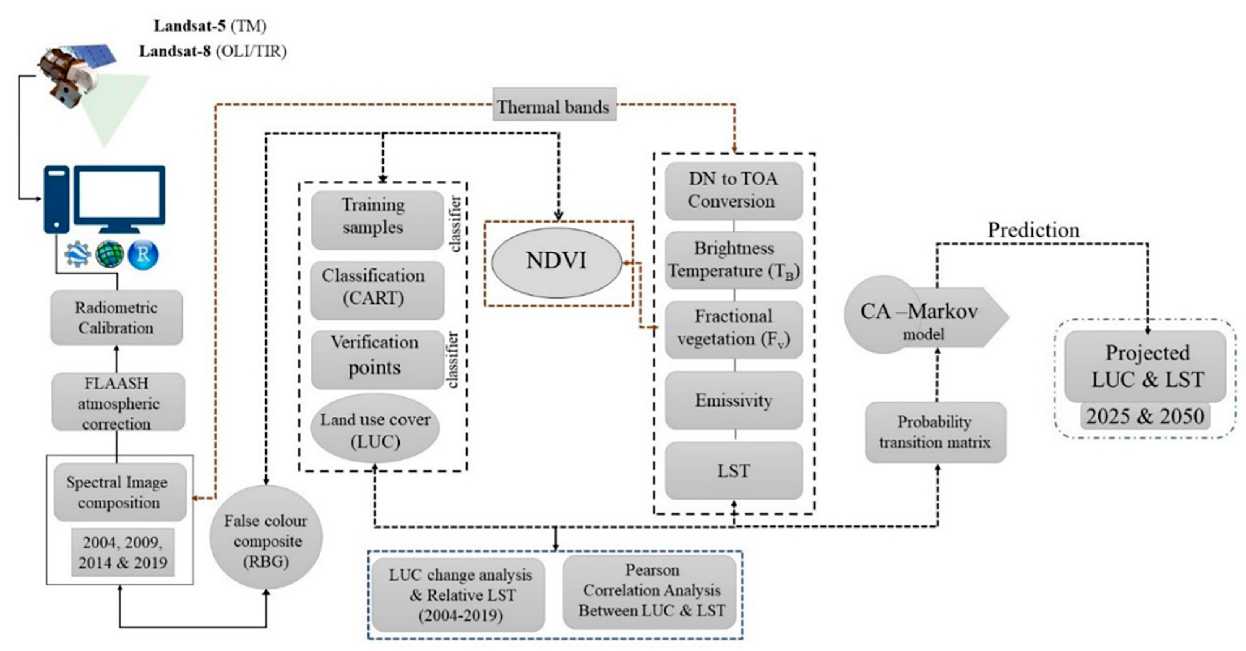
2. Material and Methodology

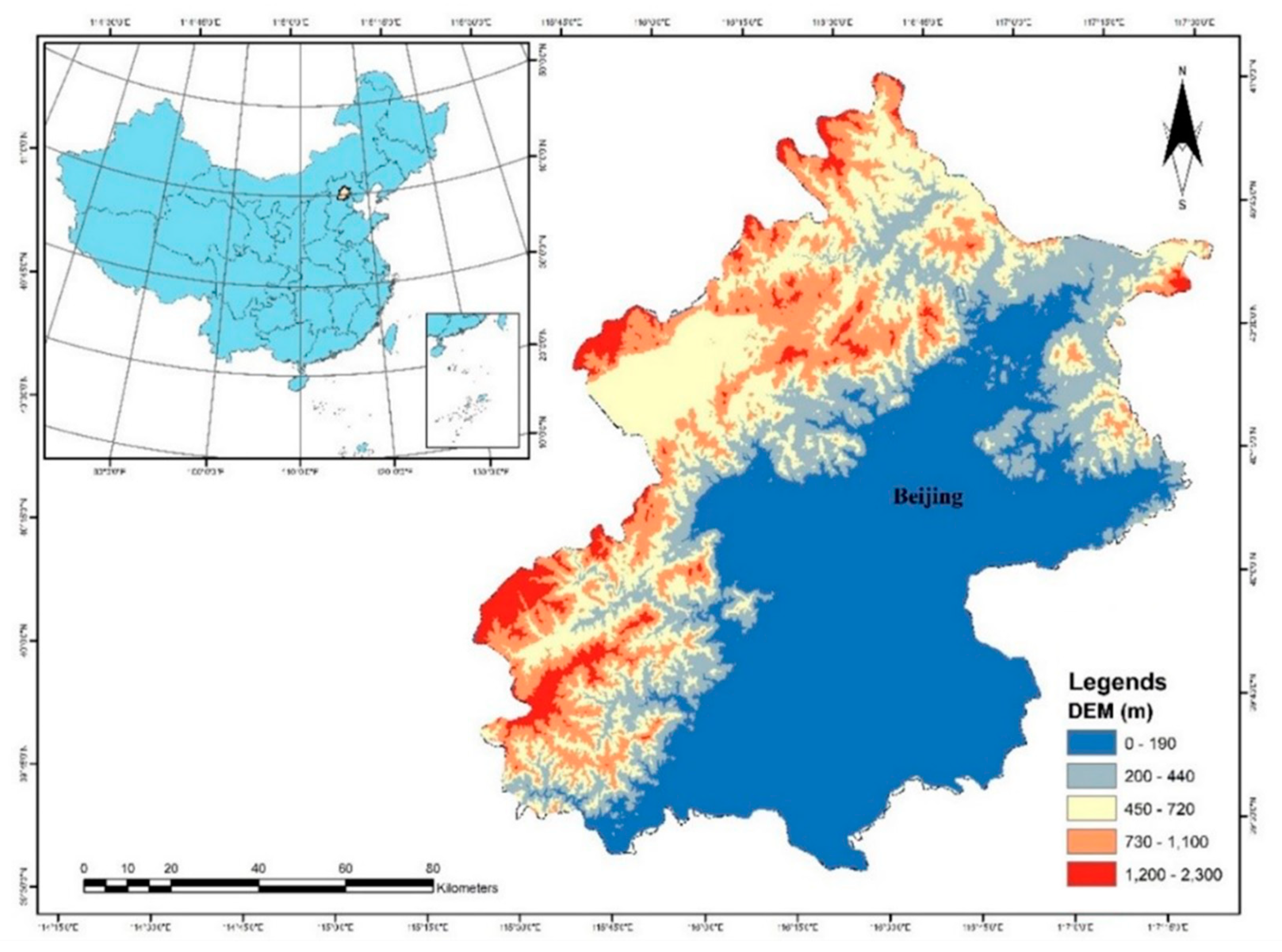
2.1. Study Area and Datasets

Beijing, the People’s Republic of China’s capital, covers 14 districts and two counties, and the total urban area is approximately 16,410.54 km2 with a population of 21.893 million (Beijing Statistics Bureau, November 2020). According to Beijing’s urban master plan (2004–2020), Beijing is divided into four functional zones [31,32,33]. The city has a sub-humid, mild tropical monsoon climate and four seasons, with a chilly, windy winter and dry, sticky summer (Figure 1). However, environmental issues in Beijing have drawn international attention. The region is experiencing sand and dust storms in spring, UHIs forming in summer, and pollution fog in winter, all arising from combinations of soil, location, drainage, sources of pollution, land utilization, and urbanization.
Spatial images of Landsat-5 (TM) and Landsat-8 OLI (ETM) having a 30 m resolution over various periods between 2004 and 2019 were obtained by using Google Earth Engine (GEE) for evaluating changes in LUCC and LST. From 2004 to 2019, the minimum cloud cover for the entire Landsat scene was chosen. They overlapped with the area of study (Table 1). Before LUCC classification, the Landsat images were pretreated to remove atmospheric effects [24,26,34,35]. For LUCC classification accuracy, a ground survey was conducted to collect 250 ground control points for each land cover class. The digital elevation model (DEM) was collected from SRTM by using GEE. Each spatial scene was enhanced using the histogram equalization approach to attain a higher image contrast [36,37].
A series of steps were completed in a step-wise workflow pattern (Figure 2). First, information sets were processed in GEE to construct a False Color Composite (FCC). The study area was extracted from all spatial imaginaries via masking of Beijing’s geo-referenced outline boundary map. The Supervised Classification method was used to improve classification results from Landsat images. Statistical inferences from the mean LST and the percentage proportion of different land cover types, vegetated and non-vegetated areas, were drawn through correlation analysis from 2004 to 2019. The CA–Markov model was applied to predict future (2025 and 2050) trends of LUCC and LST.

2.2. Land Use/Cover Change

The Supervised Classification method is an algorithmic probability program applied to land cover classification. Classification and Regression Trees (CART) [21,38,39] is a primer supervised classification algorithm used in remote sensing techniques of spectral images. Ground verification in uncertain areas was completed through Google Earth Pro and GEE, where misclassified areas were corrected by positioning and rearranging the GEE script samples. The ground truth point was used to estimate mapping accuracy. Finally, Landsat-5 (TM) and Landsat-8 OLI (ETM) were classified into six land cover types using the CART classification algorithm (Table 2).
Producers and users assessed the remote sensing image; overall, a confusion matrix was calculated for the classification accuracy and kappa coefficient. Producer precision is the number of pixels that have been correctly identified as a percentage of the classifier’s pixels as a training sample of each batch. User precision is the pixels that have been accurately categorized as percentages of the total number of pixels identified as the class. Overall classification accuracy is the ratio of the total number of pixels correctly assigned to the total number. Equation (1) defines the kappa coefficient. The number of random points used to determine accuracy for each image was 250.
K a p p a   C o e f f i c i e n t = N i m X i i i m ( X i + X + i ) N 2 i m ( X i X + i )

2.3. Calculation of Normalized Difference Vegetation Index (NDVI)

The Normalized Difference Vegetation Index (NDVI) is the most commonly used vegetation index to observe greenery globally. The Near-Infrared (NIR) and red band ratio are also used to map vegetation to test its condition using Equation (2) [40]. The magnitude of that index is between −1 and 1. For green plants, the standard range is between 0.2 and 0.8 [41].
N D V I = ( N I R R E D / N I R + R E D )
where NIR = Band 4 (For Landsat TM) and Band 5 (For Landsat 8) and RED = Band 3 (For Landsat TM and ETM) and Band 4 (For Landsat 8).

2.4. Retrieval of Land Surface Temperature (LST)

Radiometrically corrected Landsat images with a thermal infrared band (Band 6) were used to derive LST. The Digital Number (DN) was converted to at-satellite brightness temperature and corrected for equal weights of atmospheric absorption, re-emission, and surface emissivity [16,38,42,43,44]. To restore the spectral radiance to Top of Atmosphere (TOA), we used the brightness temperature beneath uniform emissivity [20,45]. The Land Surface Temperatures (LSTs) were computed using Equations (3)–(9) [16,24] (Figure 3).
L λ = 0.0003342 D N + 0.1
where Lλ is the spectral radiance in Wm−2 sr−1 mm−1.
We converted the spectral radiance to at-satellite brightness temperature (TB) under the assumption of uniform emissivity. The conversion formula is given in Equation (4).
T B = K 2 ln ( ( K 1 / L λ ) + 1 )
TB is the brightness temperature in Kelvin (K), Lλ is the spectral radiance in Wm−2 sr−1 mm−1, and K2 and K1 are calibration constants. For Landsat-8 OLI, K1 is 774.89 and K2 is 1321.08.
The fractional vegetation, Fv, of each pixel was determined from the NDVI using Equation (5) [46,47].
F v = ( N D V I N D V I m i n N D V I m a x N D V I m i n )
NDVImin’s value (0.2) and pixels considered bare soil, NDVImax is the maximum NDVI value (0.5), and pixels are regarded as healthy vegetation.
is the effect of the geometrical distribution of natural surfaces and internal reflections calculated by Equation (6).
d ε = ( 1 ε s ) ( 1 F v ) F ε v
where εv is vegetation emissivity, εs is soil emissivity, Fv is fractional vegetation, and F is a shape factor with a mean of 0.55 [16,38,46,48].
ε = ε v F v + ε s ( 1 F v ) + d ε
where ε is emissivity, and ε may be determined by Equation (8):
ε = 0.004 F v + 0.986
Finally, the LST was derived using Equation (9) [41,46,47,48]:
L S T = T B 1 + ( λ σ T B / ( h c ) ) ln ε
where λ is the effective wavelength (10.9 mm for band 10 in Landsat 8 data), σ is the Boltzmann constant (1.38 × 10⁻²³ J/K), h is Plank’s constant (6.626 × 10⁻³⁴ Js), c is the velocity of light in a vacuum (2.998 × 10⁻⁸ m/s), and ε is emissivity.

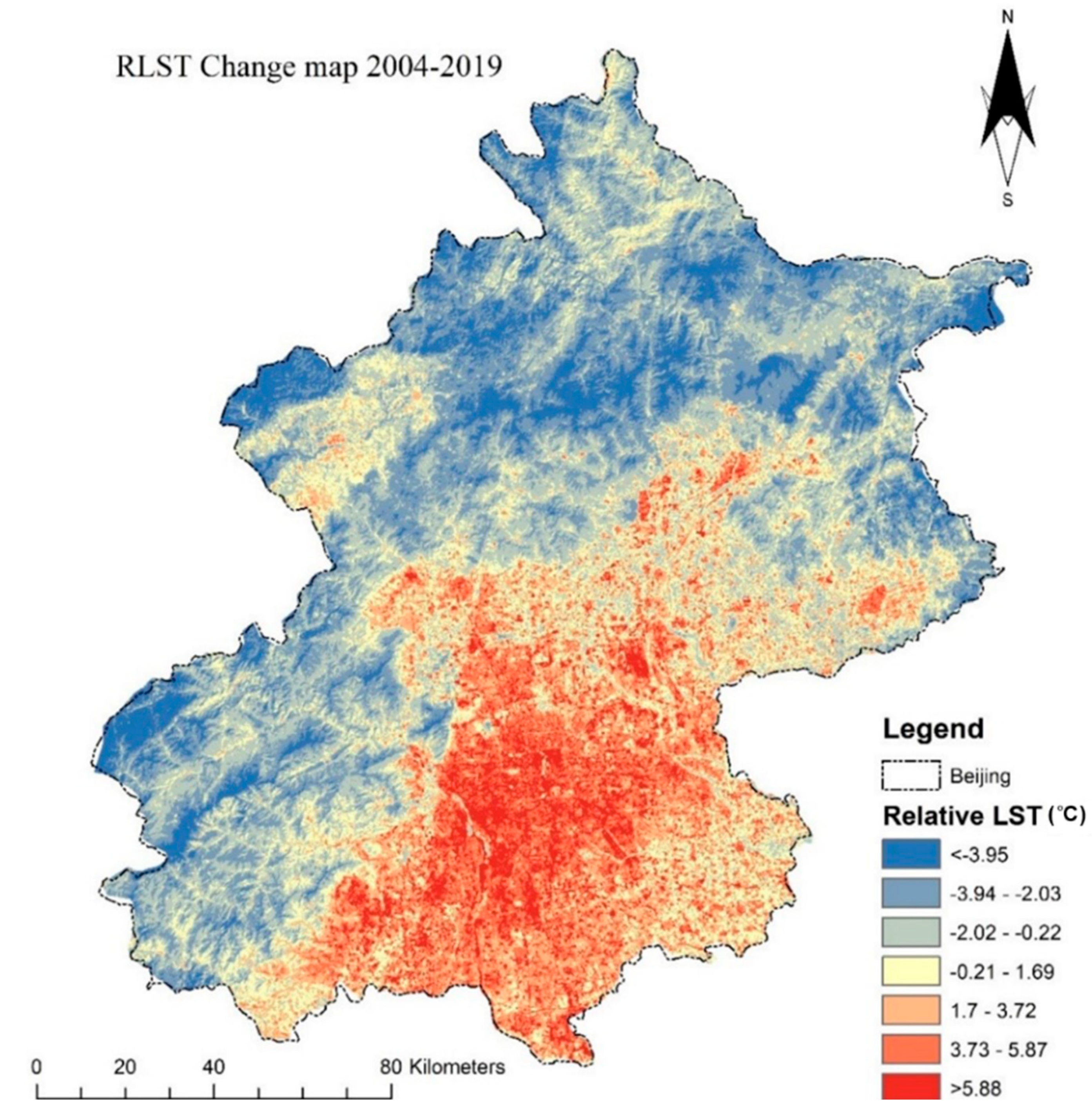
2.5. Relative LST Change Detection

For the years 2004 and 2019, the relative LST was calculated to compare the effects of LUCC on the thermal urban climate. RLST changes from LUCC (increase/decrease) are derived from the study region’s mean LST and using Equation (10) via increasing pixel value [35,44,49].
R L S T j k = L S T j k L S T j   m e a n
where RLSTjk represents the relative temperature of pixel j of class k, LSTjk is the temperature of cell j of class k, and LSTj indicates the mean value of LST for urban landscape j. If RLSTk j > 0, the pixel shows a positive contribution of LUCC conversion, and if RLSTk j < 0, then it is a negative contribution to the thermal environment.

2.6. Cellular Automata–Markov Chain (CA–Markov) Model Analysis

This model is developed based on a Markov stochastic probability matrix for predicting the transition of one status to another [26,50,51]. Generally, the Markov chain model is used to simulate transitions, parameters, and trends. It generated probability transition matrices to predict and classify potential land use/cover change (LUCC) and urban development scenarios and examined land surface temperature (LST) simulation patterns [20,52,53]. Trends were estimated using Equations (11)–(13) based on the conditional probability formula.
S ( t + 1 ) = P i j × S ( t )
P i j = ( P 11 P 21 P n 1 P 12 P 22 P n 2 P 1 n P 2 n P n 3 )
Moreover,
( 0 P i j < 1   and   j = 1 N P i j = 1 ,   ( i , j = 1 , 2 , . n ) )
where S(t) is the state of the system at time t, S ( t + 1 ) is the state of the system at the time ( t + 1 ) , and P i j is the matrix of the transition probability in a state.
The cellular automata (CA) and Markov chain model is used to calculate LUCC and LST’s future scenario by projecting 2025 and 2050. Forecasting LUCC and LST for the projected period was made through the CA–Markov model using the land use change modeler (LCM) in Terrset (Clark Labs TerrSet 18.31).

3. Results

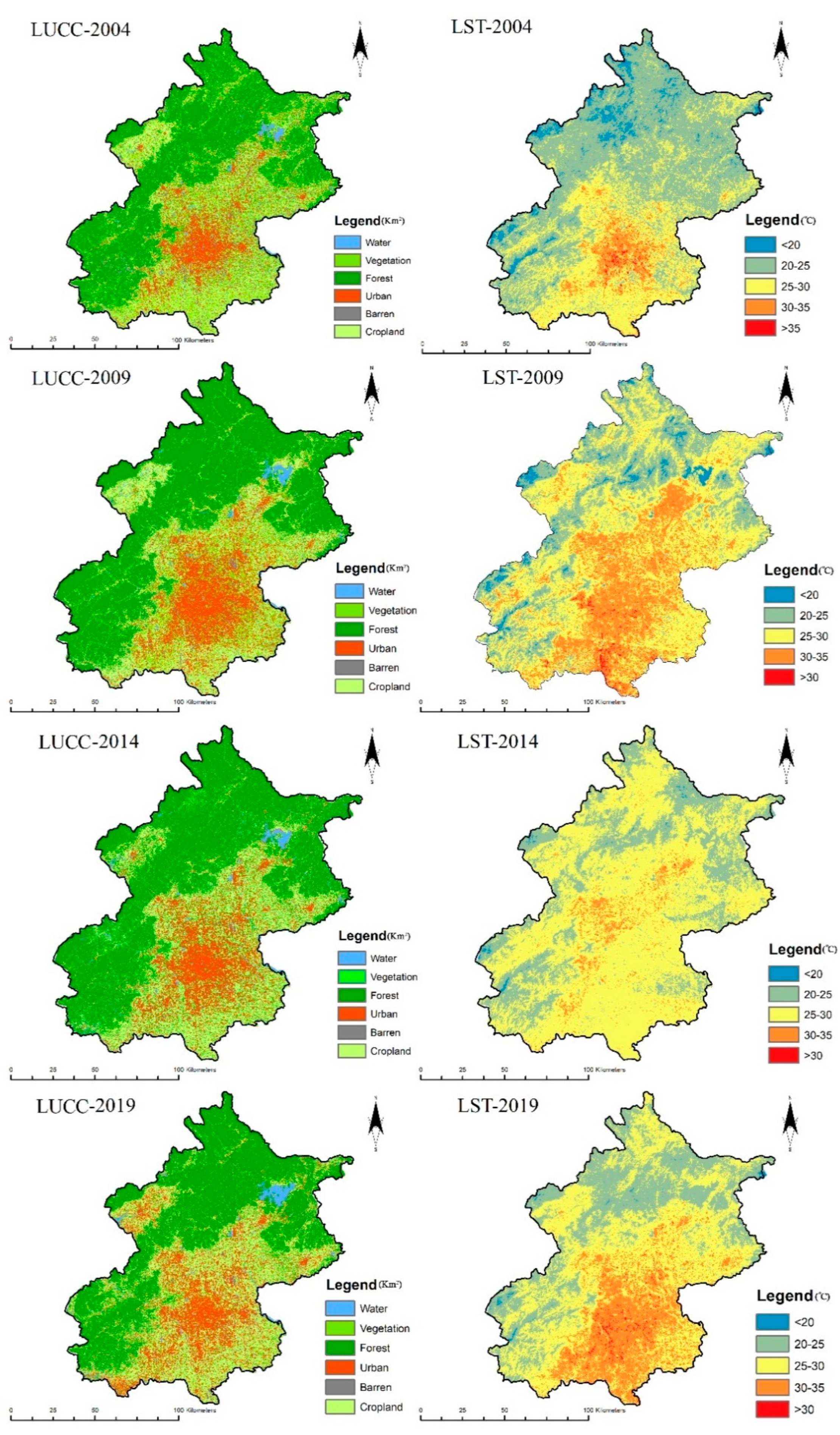
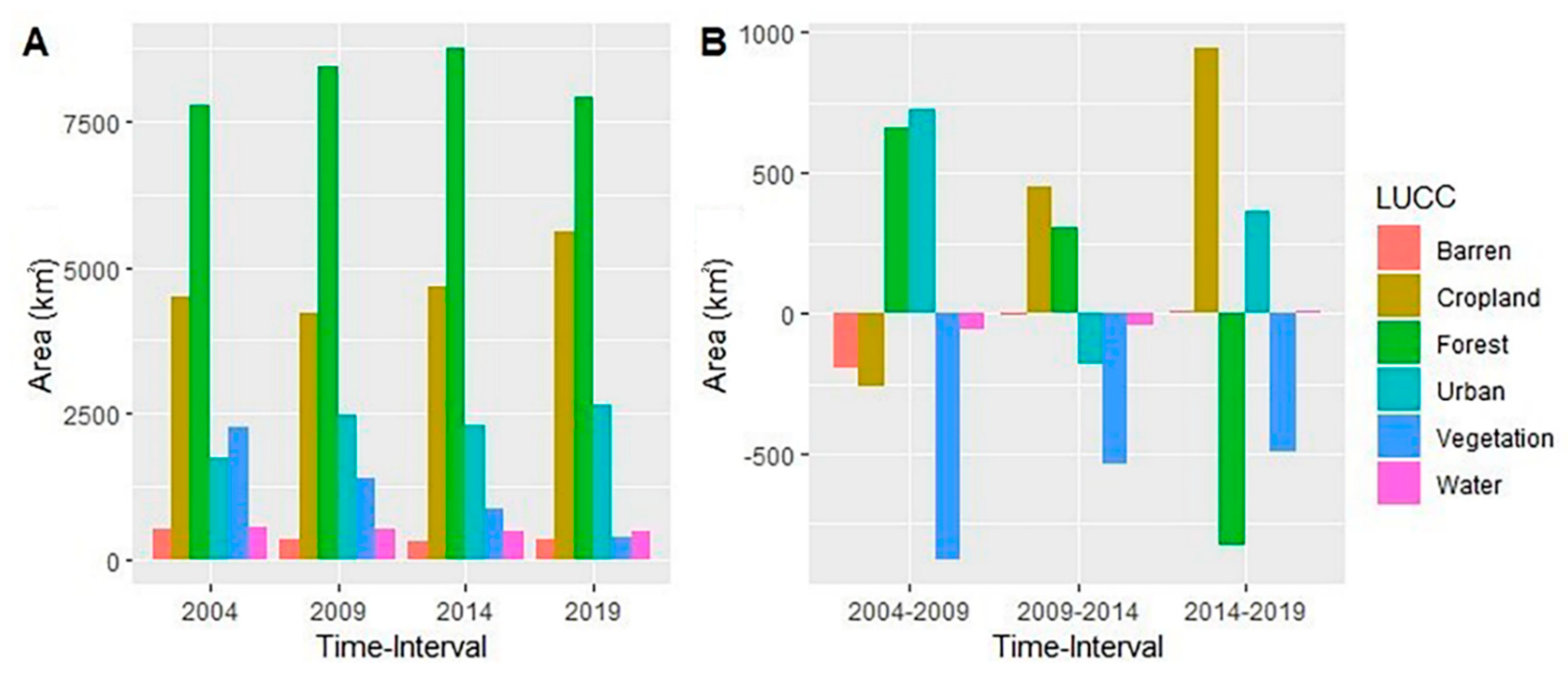
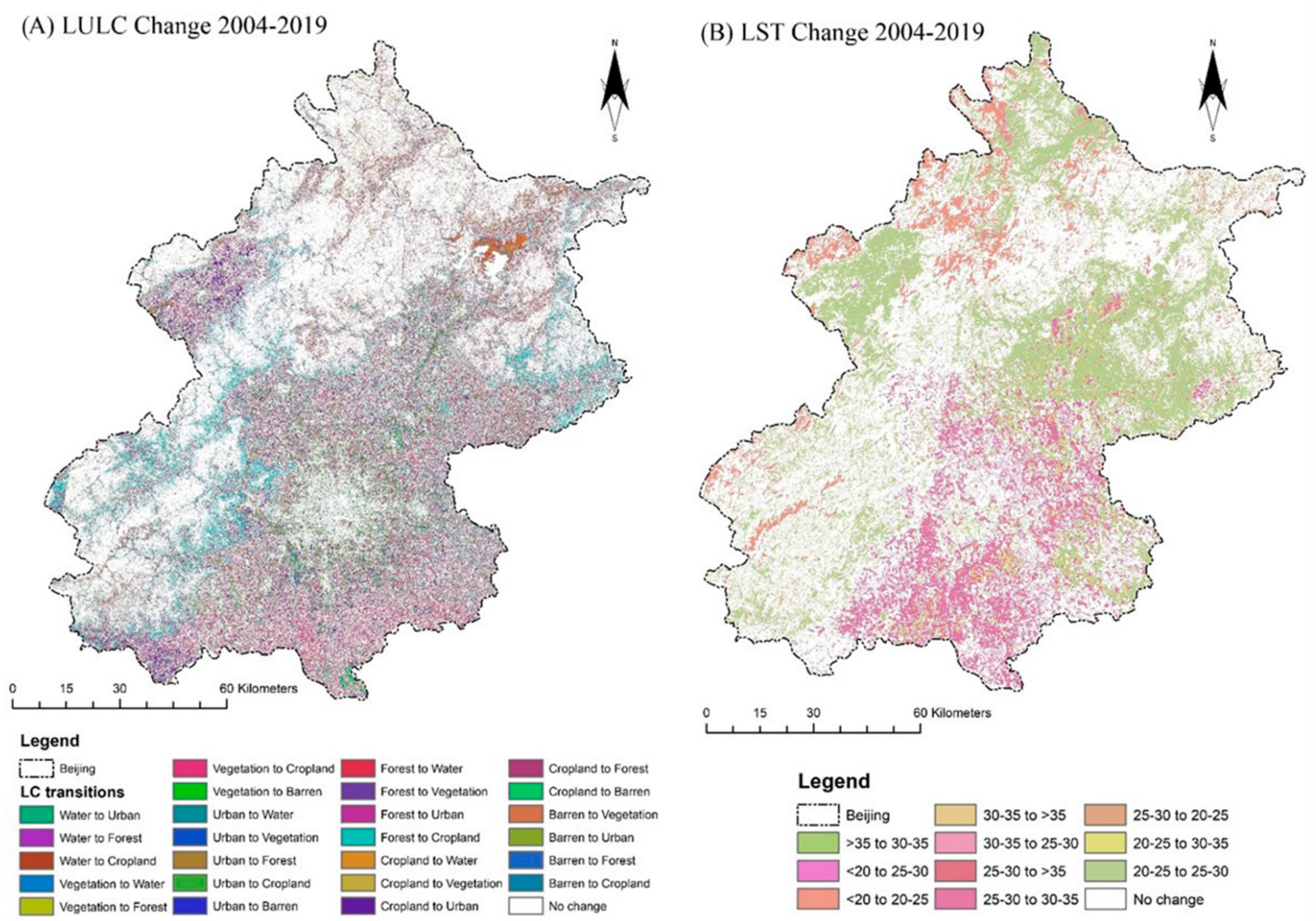
3.1. Land Use/Cover Changes (LUCC)

Land use/cover change (LUCC) was generated for the years 2004, 2009, 2014, and 2019 focusing on urban area (UA), vegetation area (VA), forest area (FA), barren land (BL), cropland (CL), and water bodies (WB). The results in Figure 3 illustrate that an area of 1743.73 km2 in 2004 and 2651.89 km2 in 2019 fell under UA’s category, indicating a cumulative change of 5% in UA of about 908.15 km2 from 2004 to 2019. The VA decreased from 2266.87 km2 to 363.57 km2 for a net decrease of 11%. WB decreased from 559.65 km2 in 2004 to 472.64 km2 in 2019, with an inverse accumulative change of 1%. FA increased from 7775.58 km2 in 2004 to 7921.90 km2 in 2019, a cumulative increase of 1% during 2004–2019. In 2004, BA was about 511.79 km2 and it was 319.81 km2 in 2019, showing an inverse change of 1%. At the same time, a 7% net increase was observed in CL from 2004 to 2019.
The kappa coefficient value was above 0.85 for all three classified images. The overall classification accuracy was 89.56%, 91.89%, 91.86%, and 94.26% for 2004, 2009, 2014, and 2019, respectively.
According to the statistics (Table 3), about 44% of the urban area remained unchanged from 2004 to 2019, while 23% loss and 33% gain were observed in LUCC types in the urban landscape. For vegetation overall, 755.10 km2 (69%) of the area was lost, 288.93 km2 (26%) was added, and 55.22 km2 (5%) of sites remained unchanged, which clearly shows the massive changes in urban vegetation.
Based on the change detection map (Figure 4A), about 61.42% of the land use area remained unchanged from 2004 to 2019. Overall, 38.58% of changes were observed in LUCC types in the city landscape, in which 3.7% were observed in CL converted into an urban area, followed by BL (1.23%) into cropland, FA (7.09%) swapped to impervious surfaces, and CL into FA (6.24%) (Figure 5). A good change was observed in the conversion of BL (1.22%) and WB (0.78%) into an urban area, cropland (0.92%) converted to urban vegetation, and 0.54% of agricultural land replaced by impervious land (Figure 4A). Additionally, a slight change was found in the conversion of WB (0.4%) into the forest area, VA (0.39%) into impervious surfaces, and BL (0.15%) into FA. Rapid anthropogenic activities have significantly replaced the natural surface area with semi-natural or impervious surfaces and other land uses between 2004 and 2019.

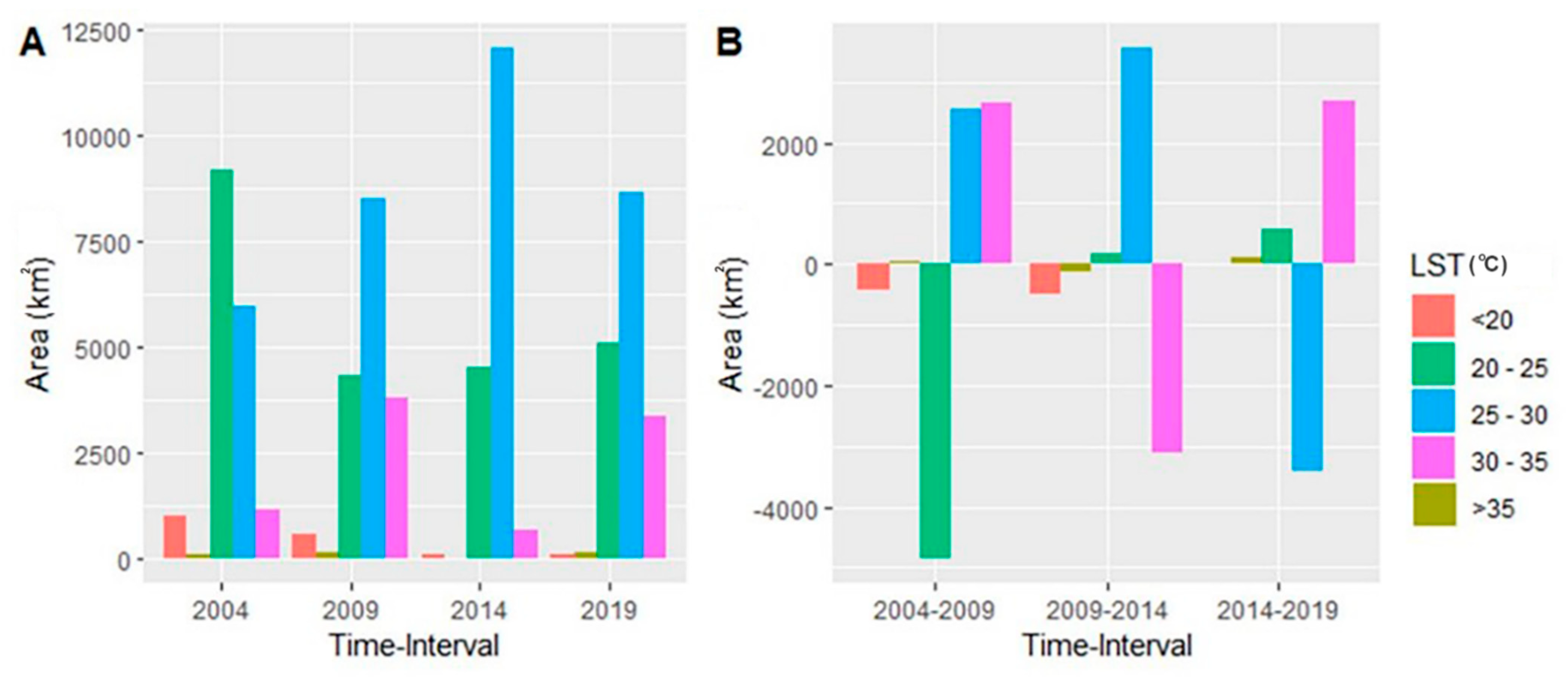
3.2. Estimation of Land Surface Temperature (LST)

Land surface temperature (LST) for Beijing city (Figure 3) was estimated with the minimal and peak value of 7.15–30.05 °C in 2004, 6.24–34.09 °C in 2009, 11.85–43.98 °C in 2014, and 15.08–43.85 °C in 2019. Generally, the mean LST investigated was 14.70 °C in 2004, whereas it peaked at 26.70 °C in 2019. Finally, the LST range is classified into five various thermal comfort zones (Table 4).
The results in Figure 5 and Figure 6 illustrate an area of 968.45 km2 in 2004 and 69.33 km2 in 2019, falling under the neutral category, indicating a cumulative change of −5% in neutral areas (<20) of about 899.12 km2 from 2004 to 2019. The slightly warm (20–25 °C) area decreased from 9158.75 km2 to 5079.99 km2 for a net decrease of 24%. The area under the warm (25–30 °C) category increased from 5940.89 km2 in 2004 to 8637.82 km2 in 2019, with an accumulative change of 16%. The hot (30–35 °C) area increased from 1137.23 km2 in 2004 to 3362.27 km2 in 2019, with a cumulative increase of 13% during 2004–2019. An area of 79.91 km2 in 2004 and 129.88 km2 in 2019 fell under the very hot category (>35 °C), indicating a cumulative change of 0.003% of about 55.98 km2 during 2004–2019.
Apart from global warming and climate change, the city’s surface temperature was minimal in 2004 because of the proliferation of green space and a low percentage of impervious surfaces spread around the city center. In 2019, the minimum and maximum surface temperatures increased due to urbanization.

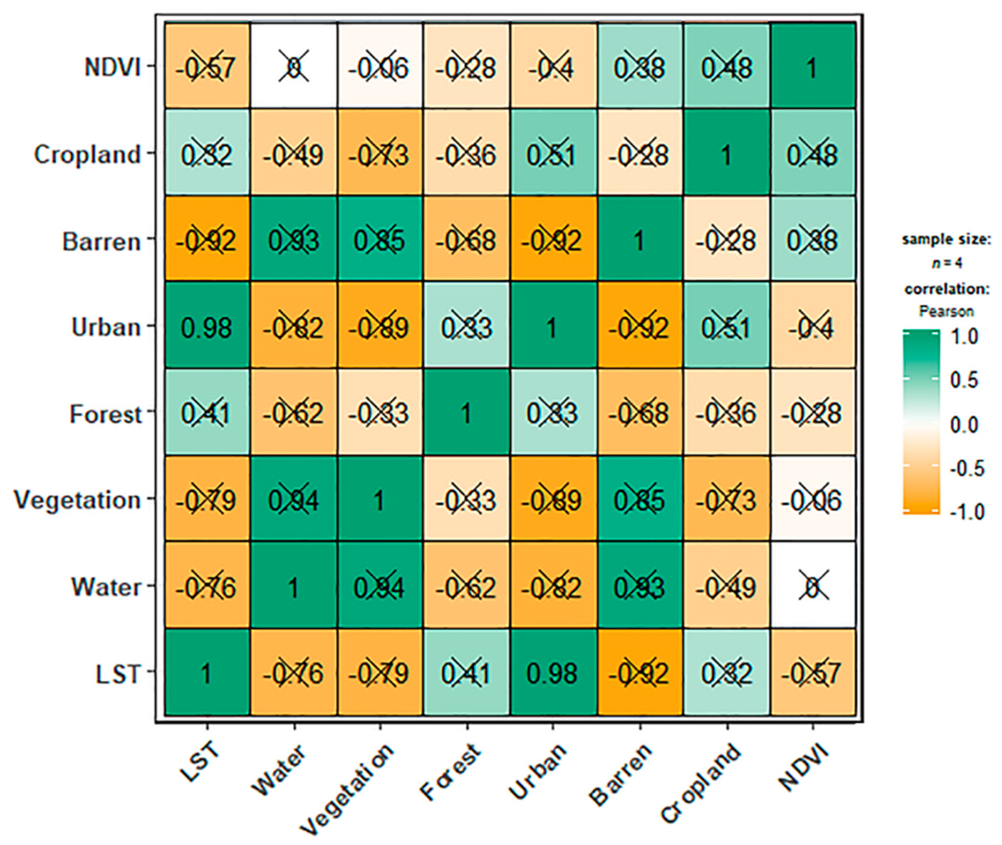
3.3. Relationship between LUCC and LST

A non-significant negative linear relationship between vegetation and land surface temperature (LST) was observed with an R-value of −0.155(p > 0.419) (Figure 7). Simultaneously, the water index showed a strong negative correlation with land surface temperature, resulting in an R-value of −0.809 (p = 0.000). A significant positive correlation between urban areas and LST was found with an R-value of 0.526 (p = 0.003).

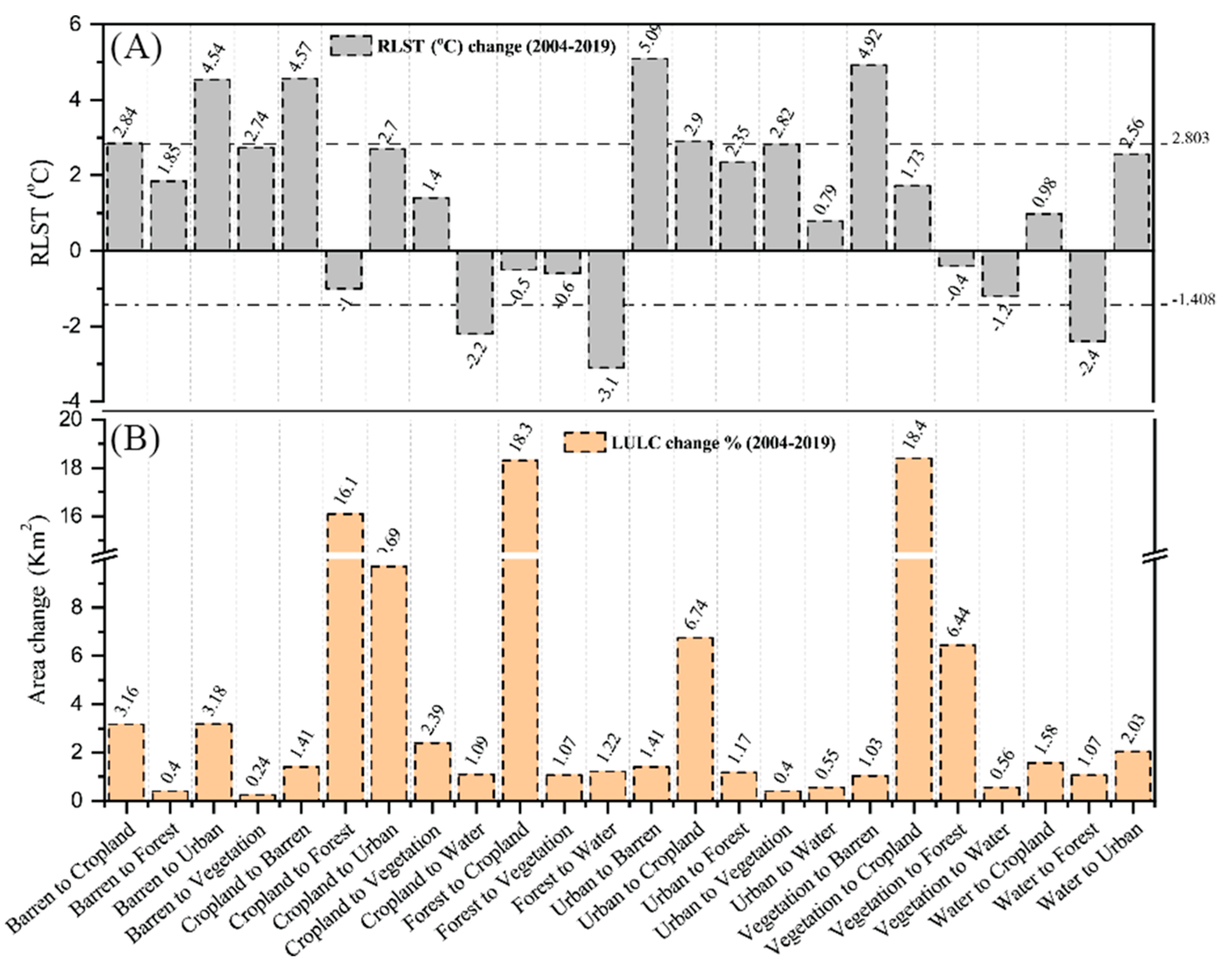
3.4. Warming and Cooling Impacts of LUCC from 2004 to 2019

LUCC had warming and cooling impacts on urban climate (Figure 8 and Figure 9). The overall maximum warming effects of 5.10 °C, 4.92 °C, and 4.58 °C were observed in the urban area (UA) transformed from barren land (BL), the vegetation area (VA), and agriculture/cropland (CL). Continued urbanization replaced BL with UA and CL, respectively, which raised the RLST by 2.90 °C and 2.84 °C. In the forest area (FA) transition by vegetation, urban, and barren areas, the mild warming effects of 2.82 °C, 2.36 °C, and 1.86 °C were quantified. The minimum positive effect on LST was noticed in the conversion of UA and CL to water bodies.
On the other side, the optimum cooling impact of about −3.20 °C, −2.28 °C, and −1.05 °C was observed in converting the urban area, cropland, and vegetation area into water bodies. A restrained decline in LST of approximately −2.41 °C, −1.05 °C, and −0.66 °C was quantified in the forest area transformed from urban, cropland, and vegetation areas.
The significant positive influence on the RLST is correlated with the transformation of forest areas into impervious and urban regions, while the cooling impact is due to BL and UA being converted into FA. We also investigated moderate changes in surface temperature in the water bodies and grass/agriculture land converted into barren land and urban counties.
The minimum cooling impact of about −0.58 °C and −0.50 °C was observed in converting FA and VA to agriculture/cropland due to the minimum difference in deciduous plantation and urban vegetation with cultivated land.

3.5. Cellular Automata–Markov Chain (CA–Markov) Model Analysis

The combination of cellular automata (CA) and the stochastic transition matrix of the Markov chain model resulted in LUCC and LST for the projected period of 2025 and 2050 (Figure 10). Map accuracy for the projected land use/cover change for predictive years was classified by the sufficient kappa coefficient value of 0.97. A decrease of 6% and 11% of forest cover areas was estimated during 2019–2025 and 2019–2050, respectively (Table 5). The urban area will expand by 5% (2019–2025) and 8% (2019–2050), adding a specific rise in relative temperature for 2025 and 2050. Urban vegetation will decrease to 482.27 km2 (3%) and 436.57 km2 (3%), and cropland will increase by 4% and 5%. Between 2019–2025 and 2019–2050, there would be little change in the increase in barren land and water bodies.
During 2019–2025, the area under the slightly warm (20–25 °C) and warm (25–30 °C) categories decreased by about 3.51% and 1.60% (Table 6), which shifted to a positive increase in the hot (30–35 °C) and very hot (>35 °C) categories up to 5.51% and 0.01%, respectively. However, this alarming shift continues under warm and slightly warm areas with a decrease of about 21.60% and 12.15%. Areas under the hot (30–35 °C) and very hot (>35 °C) categories increase by about 26.95% and 1.68%, respectively, during 2025–2050 (Table 7).

4. Discussion

4.1. Implication of Land Use/Land Cover Change for LST

Although relationships between land surface temperature (LST) and land use and cover change (LUCC) have been studied previously [26,28,54], they lack the application of remote sensing technology to infer patterns and relationship dynamics. Further, 2004 to 2019 provides a unique, nearly two-decade span of extreme growth and economic change in Beijing’s large metropolitan area. Moreover, we also simulated these parameters for 2025 and 2050 to provide future urban development plans [5,26,55]. The results provide insight into testable hypotheses, the quantities of individual contributions of LUCC to LST in hotspot areas, and potential mitigation measures to combat consequential adverse effects. The findings have shown that urban sprawl is the primary driving force in land surface temperatures (LSTs). This radiation and heat exchange is essential in rising urban heat islands (UHIs) [5,56,57]. Land use and land cover change (LUCC) impact RLST, especially in urban areas [58]. LUCC is essential to active management for awareness of anthropogenic climate change and global warming [24,26,59].
Currently, the available literature has shown that land cover classification could estimate the existing relationship between LST and LUCC [18,22]. UHIs may have been the product of some essential factors such as macro/meso-climates, urban morphology, population growth, geographical and biophysical shifts in surface area, anthropogenic changes, wind corridors, population challenges, and human lifestyles. We noticed that there was a significant trend in LUCC between 2004 and 2050.
The massive changes seen in LUCC could be attributed to Beijing’s rapid development in the 1990s and 2000s. This period was characterized by the intense deforestation and demotion of cropland for various developmental projects. Agricultural land shifted to use as impervious surfaces and built-up areas for housing and industry, characterized by a simultaneous decline in total vegetation cover (VC) [60,61]. This rapid depletion of VC has a wide range of impacts on natural cooling due to the shading and evapotranspiration provided by plants and shrubs [62,63]. To bolster this [24,64], the negative linear relationship between the Normalized Difference Vegetation Index (NDVI) and LST demonstrated that VC acts as a sink within a UHI because of its cooling effects. This change could eventually obliterate the processes of surface evaporation and transpiration in plants [65]. Previous studies have seconded this phenomenon, while its impact on LST reduction in grasslands and ornamental plants is less than in vegetation covered by forests and urban treebanks and gardens [36,66,67].
Our results elucidate that land cover has a dominant impact on LST in urban environments. The impact values of LUCC such as Urban/Built-up areas, urban vegetation, water bodies, and forests on their LST vary according to their proportional area [19,68]. Vegetation is shown to play an essential role in mitigating or controlling temperatures in urban areas [64]. Moisture is added to the surrounding air by evaporation from the top of water bodies. Previous studies have shown that water bodies play a significant role in regulating LST in residential areas [69,70]. Urban areas play an essential role in the development of urban intricate heat flows.
Our study revealed that the vegetation area was not significant since LST has been significantly influenced by growth in developed regions. This may be attributed to the upward extension of external expansion, thereby mitigating vegetation’s impact on LST. Temperature values measured in densely vegetated areas were low. In contrast, the highest LST values were observed in barren/impervious land compared to other land cover areas in various urban districts of Beijing [71]. According to previous findings, our results are primarily that Beijing’s built-up areas have a strong positive linear relationship with LST [19,61,72]. A higher temperature rise results from the increase in impervious rough, dark surfaces, including dirt, metal, and asphalt. Due to low reflection and intense solar radiation uptake, the building material increased LST, which often emits heat day and night [9,62]. This analysis shows that UHIs have a negative NDVI trajectory [73]. In addition to urban expansion, the downtown area of Beijing has undergone significant changes.
Government and private parties have revitalized a substantial amount of land for new residential, commercial, and industrial plants. This has destroyed traditional wooden houses and the architecture of rice straw roofs and tile roofs and replaced them with skyscrapers and tall buildings made with impermeable, anti-transpiring non-evaporated materials such as concrete, glass, and solid aluminum. These materials directly affect heat fluxes in urban air spaces. Previous studies have shown that LST in China is severely affected by urban rather than rural systems [73,74,75,76], similar to other countries [77,78]. The conversion of forest and agricultural land into urban territories has also contributed to the LST increase. The government has moved several factories and companies to the outskirts of cities to make them more successful in environmental health. The new factories and subsidiary infrastructures are often placed in well-conditioned agricultural or forest land, augmenting the LST of that particular zone. Historically, vegetation or forested areas were considered a fringe line between urban and rural areas to absorb excess heat generated by automobiles and factories harbored within city limits [6,78].
These results work in concert to establish urban sprawl as the primary factor producing an abnormal heat-flux and impacting LST. This radiation and heat exchange is considered a significant effect in UHIs, which causes a substantial contribution to climate change in the city canyon. While LUCC broadly has an intense impact on the relative LST, anthropogenically induced LUCC increases RLST within the urban micro-atmosphere [38].

4.2. Land Use Conversion and Its Contribution to UHIs

The land use/land cover changes and associated RLST demonstrate the urban climate’s positive and negative contributions at the standardized scale (10%). For example, this study reveals that barren land’s transition into metropolitan areas contributes 1.01% to UHIs. In comparison, the warming effect is 1.23% in converting the 0.59% area, which is higher than the warming effect. The reasons for such surprising findings may be the locations of the LUCC close to water bodies and forest land. On the other hand, the conversion of the same area of 0.15% barren land into forest areas contributes a warming effect of 0.41% to UHIs. Similarly, the transition of barren land into vegetation areas pays about 0.61% to UHIs, while the negative input is −0.07 in reverse change (Table 8).
The overall contribution is higher than the contribution for ventilation, owing to low to high surface energy. The results show that the warming contribution of the natural surface to the impervious surface is much more significant than the cooling contribution. Overall, this study showed that the maximum contribution to warming is caused by vegetation change, particularly urban forests, to high LST impervious areas. Simultaneously, the minimum result is converting from an impervious surface to grass/agricultural land with minimal surface temperature variation. This reveals that increasing green spaces in urban regions could benefit the urban climate. Simultaneously, the developed sites and impervious parts have low heat transmission capacity and trapped solar energy that can boast the UHI/thermal climate.
Recent scientific literature [47] concluded that the overall contribution of up to ~65% warming impact associated with LUCC is well-matched with the expected warming effect due to physical interaction across the Indian region, which supports our findings.
Indeed, the maximum cooling contribution is 0.23% in converting forest areas into water bodies in the land use dynamic process. In comparison, the minimum cooling effect of 0.04% was observed from vegetation change to forests. The purpose behind the least contribution of vegetation area is the minimal difference in surface temperature and proximity to the impervious surface. Meanwhile, the highest cooling is investigated in the conversion of forest areas to water bodies. At the same time, the most negligible impact is obtained from the transformation of vegetation areas to forest land. Some land cover’s cooling contribution is changed into an urban area, forest area, water bodies, vegetation, and crop/agriculture land.
Similarly, the inadequate literature on LUCC, associated relative land surface temperature, and their percent contribution makes it hard to make the correct analogy. Recently, a study also seconded our findings by concluding the impact of LUCC on surface temperature and the percent contribution in LST related to LUCC in Donating Lake Area, China [48].

5. Conclusions

The present study evaluated LUCC’s influence on the LST in a large urban area of Beijing, observing the developmental resolution and different socio-economic parameters using RS data. This research established a link between LST and the urban environment. Using coefficient and projections analysis, landscape dynamics’ contribution to temperature was evaluated using the Pearson correlation and CA–Markov model. It was discovered that increasing the built-up area by 5% increased the temperature by 1%. Increases in vegetation cover of 10% had a negative correlation as well. For the study period of 2019 to 2050, the rise in land surface temperature (LST) was 7.5 °C (10.35%). Overall, the findings reveal the average warming effect of 2.80 °C and the average cooling effect of −1.41 °C of LUCC in Beijing from 2004 to 2019. Due to forest land transformation to impervious surfaces, the average warming contribution of LUCC to UHI is 0.5%. In comparison, 0.11% cooling was found in reverse direction shifts. The positive contribution in UHIs due to the conversion of forest land into impervious surfaces is higher than the negative contribution.
More targeted green efforts should be placed on urban design, infrastructure planning, and development to negate temperature increases. Enhancing water bodies such as lakes, canals, waterfalls, and fountains and a significant increase in green spaces such as artificial parks, gardens, the linear plantation of woody plants, and the promotion of open-concept areas are all part of this plan. This study indicates that more extensive research is urgently required to assess changing land use/cover on local and regional climate. Many areas are rapidly changing due to the expanding effects of modern climate change and progressive activity. The geographic environment and known weather patterns of Beijing should be harnessed to promote natural cooling processes. In amalgamation, environmental education should be accessible to encourage ecological development concerning resource planning and management. Hence, there is a greater need for green policy intervention and effective urban planning to control the soaring thermal environment. A quantitative examination of these parameters should be included in a prospective study.
Additionally, while we discovered that urbanization has a direct effect on LST, the inverse relationship will reveal the extent to which urbanization affects LST. Future research should focus on quantifying the impacts of urbanization on LST. This study suggests intensive research in the future, specifically investigating the proportion of green space and impervious surfaces and its effects on RLST for sustainable future cities. The present study provides practical implications for urban landscape planning that requires the rational use of landscape connectivity between green and impervious surfaces and their impact on LST. Future urban research could focus on the issue of public health and infrastructure burden associated with rapid urbanization.

Author Contributions

Conceptualization and methodology, M.A.S. and P.Z.; software, M.A.S.; validation, M.A.S. and Y.W.; formal analysis; investigation, M.A.S.; resources, P.Z. and Y.W.; data curation, M.A.S. and N.U.; writing—original draft preparation, M.A.S.; writing—review and editing, M.A.S. and Y.W.; visualization, M.A.S. and N.X.; supervision. P.Z. All authors have read and agreed to the published version of the manuscript.

Funding

This work is funded by the National Natural Science Foundation of China’s (Grant Numbers 51978447) study on the response mechanism between the evolution of urbanization policy and the development of rural space networks in the Beijing–Tianjin–Hebei region.

Institutional Review Board Statement

Not applicable.

Informed Consent Statement

Not applicable.

Data Availability Statement

The authors will provide the data of this research upon request.

Acknowledgments

The authors would like to express their respect and gratitude to Bébio Amaro and the anonymous reviewers and editors for their valuable comments and suggestions to improve the quality of this paper.

Conflicts of Interest

The authors declare no conflict of interest.

References

  1. Foley, J.A.; DeFries, R.; Asner, G.P.; Barford, C.; Bonan, G.; Carpenter, S.R.; Chapin, F.S.; Coe, M.T.; Daily, G.C.; Gibbs, H.K. Global consequences of land use. Science 2005, 309, 570–574. [Google Scholar] [CrossRef] [PubMed] [Green Version]
  2. Beckline, M.; Yujun, S.; Yvette, B.; John, A.B.; Mor-Achankap, B.; Saeed, S.; Richard, T.; Wose, J.; Paul, C. Perspectives of remote sensing and GIS applications in tropical forest management. Am. J. Agric. For. 2017, 5, 33–39. [Google Scholar] [CrossRef] [Green Version]
  3. Lambin, E.F.; Geist, H.J.; Lepers, E. Dynamics of land-use and land-cover change in tropical regions. Annu. Rev. Environ. Resour. 2003, 28, 205–241. [Google Scholar] [CrossRef] [Green Version]
  4. Hersperger, A.M.; Gennaio, M.-P.; Verburg, P.H.; Bürgi, M. Linking land change with driving forces and actors: Four conceptual models. Ecol. Soc. 2010, 15, 1–17. [Google Scholar] [CrossRef] [Green Version]
  5. Zhang, Q.; Su, S. Determinants of urban expansion and their relative importance: A comparative analysis of 30 major metropolitans in China. Habitat Int. 2016, 58, 89–107. [Google Scholar] [CrossRef]
  6. Huang, Y.; Qiu, Q.; Sheng, Y.; Min, X.; Cao, Y. Exploring the Relationship between Urbanization and the Eco-Environment: A Case Study of Beijing. Sustainability 2019, 11, 6298. [Google Scholar] [CrossRef] [Green Version]
  7. Debbage, N.; Shepherd, J.M. The urban heat island effect and city contiguity. Comput. Environ. Urban Syst. 2015, 54, 181–194. [Google Scholar] [CrossRef]
  8. Sexton, J.O.; Song, X.-P.; Huang, C.; Channan, S.; Baker, M.E.; Townshend, J.R. Urban growth of the Washington, DC-Baltimore, MD metropolitan region from 1984 to 2010 by annual, Landsat-based estimates of impervious cover. Remote Sens. Environ. 2013, 129, 42–53. [Google Scholar] [CrossRef]
  9. Buyadi, S.N.A.; Mohd, W.M.N.W.; Misni, A. Impact of land use cover changes on the surface temperature distribution of area surrounding the National Botanic Garden, Shah Alam. Procedia-Soc. Behav. Sci. 2013, 101, 516–525. [Google Scholar] [CrossRef] [Green Version]
  10. Chen, X.-L.; Zhao, H.-M.; Li, P.-X.; Yin, Z.-Y. Remote sensing image-based analysis of the relationship between urban heat island and land use/cover changes. Remote Sens. Environ. 2006, 104, 133–146. [Google Scholar] [CrossRef]
  11. Tonkaz, T.; Çetin, M. Effects of urbanization and land-use type on monthly extreme temperatures in a developing semi-arid region, Turkey. J. Arid Environ. 2007, 68, 143–158. [Google Scholar] [CrossRef]
  12. Carlson, T.N.; Arthur, S.T. The impact of land use—Land cover changes due to urbanization on surface microclimate and hydrology: A satellite perspective. Global Planet. Chang. 2000, 25, 49–65. [Google Scholar] [CrossRef]
  13. Huff, F.; Changnon, S., Jr. Climatological assessment of urban effects on precipitation at St. Louis. J. Appl. Meteorol. 1972, 11, 823–842. [Google Scholar] [CrossRef] [Green Version]
  14. Almazroui, M.; Islam, M.N.; Jones, P. Urbanization effects on the air temperature rise in Saudi Arabia. Clim. Chang. 2013, 120, 109–122. [Google Scholar] [CrossRef]
  15. Li, Y.; Zhu, L.; Zhao, X.; Li, S.; Yan, Y. Urbanization impact on temperature change in China with emphasis on land cover change and human activity. J. Clim. 2013, 26, 8765–8780. [Google Scholar] [CrossRef]
  16. Sobrino, J.A.; Jiménez-Muñoz, J.C.; Paolini, L. Land surface temperature retrieval from LANDSAT TM 5. Remote Sens. Environ. 2004, 90, 434–440. [Google Scholar] [CrossRef]
  17. Feng, H.; Liu, H.; Wu, L. Monitoring the relationship between the land surface temperature change and urban growth in Beijing, China. IEEE J. Sel. Top. Appl. Earth Obs. Remote Sens. 2014, 7, 4010–4019. [Google Scholar] [CrossRef]
  18. Walawender, J.P.; Szymanowski, M.; Hajto, M.J.; Bokwa, A. Land surface temperature patterns in the urban agglomeration of Krakow (Poland) derived from Landsat-7/ETM+ data. Pure Appl. Geophys. 2014, 171, 913–940. [Google Scholar] [CrossRef] [Green Version]
  19. Verburg, P.H.; Veldkamp, A.; Willemen, L.; Overmars, K.P.; Castella, J.-C. Landscape level analysis of the spatial and temporal complexity of land-use change. Ecosyst. Land Use Geogr. Monogr. Ser. 2004, 153, 217–230. [Google Scholar]
  20. Cristóbal, J.; Jiménez-Muñoz, J.; Prakash, A.; Mattar, C.; Skoković, D.; Sobrino, J. An Improved Single-Channel Method to Retrieve Land Surface Temperature from the Landsat-8 Thermal Band. Remote Sens. 2018, 10, 431. [Google Scholar] [CrossRef] [Green Version]
  21. Ding, H.; Shi, W. Land-use/land-cover change and its influence on surface temperature: A case study in Beijing City. Int. J. Remote Sens. 2013, 34, 5503–5517. [Google Scholar] [CrossRef]
  22. Connors, J.P.; Galletti, C.S.; Chow, W.T. Landscape configuration and urban heat island effects: Assessing the relationship between landscape characteristics and land surface temperature in Phoenix, Arizona. Landsc. Ecol. 2013, 28, 271–283. [Google Scholar] [CrossRef]
  23. Amiri, R.; Weng, Q.; Alimohammadi, A.; Alavipanah, S.K. Spatial-temporal dynamics of land surface temperature in relation to fractional vegetation cover and land use/cover in the Tabriz urban area, Iran. Remote Sens. Environ. 2009, 113, 2606–2617. [Google Scholar] [CrossRef]
  24. Amir Siddique, M.; Dongyun, L.; Li, P.; Rasool, U.; Ullah Khan, T.; Javaid Aini Farooqi, T.; Wang, L.; Fan, B.; Rasool, M.A. Assessment and simulation of land use and land cover change impacts on the land surface temperature of Chaoyang District in Beijing, China. PeerJ 2020, 8, e9115. [Google Scholar] [CrossRef]
  25. Santé, I.; García, A.M.; Miranda, D.; Crecente, R. Cellular automata models for the simulation of real-world urban processes: A review and analysis. Landsc. Urban Plan. 2010, 96, 108–122. [Google Scholar] [CrossRef]
  26. Ullah, S.; Tahir, A.A.; Akbar, T.A.; Hassan, Q.K.; Dewan, A.; Khan, A.J.; Khan, M. Remote Sensing-Based Quantification of the Relationships between Land Use Land Cover Changes and Surface Temperature over the Lower Himalayan Region. Sustainability 2019, 11, 5492. [Google Scholar] [CrossRef] [Green Version]
  27. Zenil, H. Compression-based investigation of the dynamical properties of cellular automata and other systems. arXiv 2009, arXiv:0910.4042. [Google Scholar] [CrossRef]
  28. Civco, D.L. Artificial neural networks for land-cover classification and mapping. Int. J. Geogr. Inf. Sci. 1993, 7, 173–186. [Google Scholar] [CrossRef]
  29. Agarwal, C.; Green, G.M.; Grove, J.M.; Evans, T.P.; Schweik, C.M. A review and assessment of land-use change models: Dynamics of space, time, and human choice. In General Technical Report (GTR). NE-297; Department of Agriculture: Newton Square, PA, USA, 2002; p. 297. [Google Scholar]
  30. Artis, D.A.; Carnahan, W.H. Survey of emissivity variability in thermography of urban areas. Remote Sens. Environ. 1982, 12, 313–329. [Google Scholar] [CrossRef]
  31. Wu, Q.; Tan, J.; Guo, F.; Li, H.; Chen, S. Multi-Scale Relationship between Land Surface Temperature and Landscape Pattern Based on Wavelet Coherence: The Case of Metropolitan Beijing, China. Remote Sens. 2019, 11, 3021. [Google Scholar] [CrossRef] [Green Version]
  32. Tian, G.; Wu, J.; Yang, Z. Spatial pattern of urban functions in the Beijing metropolitan region. Habitat Int. 2010, 34, 249–255. [Google Scholar] [CrossRef]
  33. Qiao, Z.; Tian, G.; Xiao, L. Diurnal and seasonal impacts of urbanization on the urban thermal environment: A case study of Beijing using MODIS data. ISPRS J. Photogramm. Remote Sens. 2013, 85, 93–101. [Google Scholar] [CrossRef]
  34. Landsat. Science Data Users Handbook; Landsat: Sioux Falls, SD, USA, 2007. [Google Scholar]
  35. Sadiq Khan, M.; Ullah, S.; Sun, T.; Rehman, A.U.R.; Chen, L. Land-Use/Land-Cover Changes and Its Contribution to Urban Heat Island: A Case Study of Islamabad, Pakistan. Sustainability 2020, 12, 3861. [Google Scholar] [CrossRef]
  36. Chen, B.; Zhang, X.; Tao, J.; Wu, J.; Wang, J.; Shi, P.; Zhang, Y.; Yu, C. The impact of climate change and anthropogenic activities on alpine grassland over the Qinghai-Tibet Plateau. Agric. For. Meteorol. 2014, 189, 11–18. [Google Scholar] [CrossRef]
  37. Wu, L.; Sun, B.; Zhou, S.; Huang, S.-E.; Zhao, Q. A new fusion technique of remote sensing images for land use/cover. Pedosphere 2004, 14, 187–194. [Google Scholar]
  38. Jiang, J.; Tian, G. Analysis of the impact of land use/land cover change on land surface temperature with remote sensing. Procedia Environ. Sci. 2010, 2, 571–575. [Google Scholar] [CrossRef] [Green Version]
  39. Sang, X.; Guo, Q.; Wu, X.; Fu, Y.; Xie, T.; He, C.; Zang, J. Intensity and Stationarity Analysis of Land use cover change based on CART Algorithm. Sci. Rep. 2019, 9, 12279. [Google Scholar] [CrossRef] [PubMed] [Green Version]
  40. Elvidge, C.D.; Chen, Z. Comparison of broad-band and narrow-band red and near-infrared vegetation indices. Remote Sens. Environ. 1995, 54, 38–48. [Google Scholar] [CrossRef]
  41. Wang, R.; Hou, H.; Murayama, Y.; Derdouri, A. Spatiotemporal Analysis of Land Use/Cover Patterns and Their Relationship with Land Surface Temperature in Nanjing, China. Remote Sens. 2020, 12, 440. [Google Scholar] [CrossRef] [Green Version]
  42. Sobrino, J.A.; Jiménez-Muñoz, J.C. Minimum configuration of thermal infrared bands for land surface temperature and emissivity estimation in the context of potential future missions. Remote Sens. Environ. 2014, 148, 158–167. [Google Scholar] [CrossRef]
  43. Snyder, W.C.; Wan, Z.; Zhang, Y.; Feng, Y.-Z. Classification-based emissivity for land surface temperature measurement from space. Int. J. Remote Sens. 1998, 19, 2753–2774. [Google Scholar] [CrossRef]
  44. Qiao, Z.; Liu, L.; Qin, Y.; Xu, X.; Wang, B.; Liu, Z. The Impact of Urban Renewal on Land Surface Temperature Changes: A Case Study in the Main City of Guangzhou, China. Remote Sens. 2020, 12, 794. [Google Scholar] [CrossRef] [Green Version]
  45. Guha, S.; Govil, H.; Dey, A.; Gill, N. Analytical study of land surface temperature with NDVI and NDBI using Landsat 8 OLI and TIRS data in Florence and Naples city, Italy. Eur. J. Remote Sens. 2018, 51, 667–678. [Google Scholar] [CrossRef]
  46. Singh, P.; Kikon, N.; Verma, P. Impact of land use cover change and urbanization on urban heat island in Lucknow city, Central India. A remote sensing based estimate. Sustain. Cities Soc. 2017, 32, 100–114. [Google Scholar] [CrossRef]
  47. Zhang, Y.; Yu, T.; Gu, X.; Zhang, Y.; Chen, L. Land surface temperature retrieval from CBERS-02 IRMSS thermal infrared data and its applications in quantitative analysis of urban heat island effect. J. Remote Sens.-Beijing 2006, 10, 789. [Google Scholar]
  48. Tariq, A.; Riaz, I.; Ahmad, Z.; Yang, B.; Amin, M.; Kausar, R.; Andleeb, S.; Farooqi, M.A.; Rafiq, M. Land surface temperature relation with normalized satellite indices for the estimation of spatio-temporal trends in temperature among various land use land cover classes of an arid Potohar region using Landsat data. Environ. Earth Sci. 2019, 79, 1–15. [Google Scholar] [CrossRef]
  49. Muller, M.R.; Middleton, J. A Markov model of land-use change dynamics in the Niagara Region, Ontario, Canada. Landsc. Ecol. 1994, 9, 151–157. [Google Scholar]
  50. Zhou, L.; Dang, X.; Sun, Q.; Wang, S. Multi-scenario simulation of urban land change in Shanghai by random forest and CA–Markov model. Sustain. Cities Soc. 2020, 55, 102045. [Google Scholar] [CrossRef]
  51. Al-sharif, A.A.; Pradhan, B. Monitoring and predicting land use cover change in Tripoli Metropolitan City using an integrated Markov chain and cellular automata models in GIS. Arab. J. Geosci. 2014, 7, 4291–4301. [Google Scholar] [CrossRef]
  52. Halmy, M.W.A.; Gessler, P.E.; Hicke, J.A.; Salem, B.B. Land use/land cover change detection and prediction in the north-western coastal desert of Egypt using Markov-CA. Appl. Geogr. 2015, 63, 101–112. [Google Scholar] [CrossRef]
  53. Li, X.; Li, W.; Middel, A.; Harlan, S.L.; Brazel, A.J.; Turner Ii, B. Remote sensing of the surface urban heat island and land architecture in Phoenix, Arizona: Combined effects of land composition and configuration and cadastral-demographic-economic factors. Remote Sens. Environ. 2016, 174, 233–243. [Google Scholar] [CrossRef] [Green Version]
  54. Sejati, A.W.; Buchori, I.; Rudiarto, I. The spatio-temporal trends of urban growth and surface urban heat islands over two decades in the Semarang Metropolitan Region. Sustain. Cities Soc. 2019, 46, 101432. [Google Scholar] [CrossRef]
  55. Zhang, X.; Zhong, T.; Feng, X.; Wang, K. Estimation of the relationship between vegetation patches and urban land surface temperature with remote sensing. Int. J. Remote Sens. 2009, 30, 2105–2118. [Google Scholar] [CrossRef]
  56. Pal, S.; Ziaul, S. Detection of land use and land cover change and land surface temperature in English Bazar urban centre. Egypt. J. Remote Sens. Space Sci. 2017, 20, 125–145. [Google Scholar] [CrossRef] [Green Version]
  57. Tali, J.; Emtehani, M.; Murthy, K.; Nagendra, H. Future Threats to CBD: A Case Study of Bangalore CBD. N. Y. Sci. J. 2012, 5, 22–27. [Google Scholar]
  58. Turner, B.L.; Lambin, E.F.; Reenberg, A. The emergence of land change science for global environmental change and sustainability. Proc. Natl. Acad. Sci. USA 2007, 104, 20666–20671. [Google Scholar] [CrossRef] [PubMed] [Green Version]
  59. Chen, W.; Zhang, Y.; Pengwang, C.; Gao, W. Evaluation of urbanization dynamics and its impacts on surface heat islands: A case study of Beijing, China. Remote Sens. 2017, 9, 453. [Google Scholar] [CrossRef] [Green Version]
  60. Cai, G.; Du, M.; Xue, Y. Monitoring of urban heat island effect in Beijing combining ASTER and TM data. Int. J. Remote Sens. 2011, 32, 1213–1232. [Google Scholar] [CrossRef]
  61. Oluseyi, I.O.; Fanan, U.; Magaji, J. An evaluation of the effect of land use/cover change on the surface temperature of Lokoja town, Nigeria. Afr. J. Environ. Sci. Technol. 2009, 3, 86–90. [Google Scholar]
  62. Macarof, P.; Statescu, F. Comparasion of NDBI and NDVI as Indicators of Surface Urban Heat Island Effect in Landsat 8 Imagery: A Case Study of Iasi. Present Environ. Sustain. Dev. 2017, 11, 141. [Google Scholar] [CrossRef] [Green Version]
  63. Weng, Q.; Lu, D.; Schubring, J. Estimation of land surface temperature-vegetation abundance relationship for urban heat island studies. Remote Sens. Environ. 2004, 89, 467–483. [Google Scholar] [CrossRef]
  64. Faqe Ibrahim, G. Urban land use land cover changes and their effect on land surface temperature: Case study using Dohuk City in the Kurdistan Region of Iraq. Climate 2017, 5, 13. [Google Scholar] [CrossRef] [Green Version]
  65. Weng, Q.; Lo, C. Spatial analysis of urban growth impacts on vegetative greenness with Landsat TM data. Geocarto Int. 2001, 16, 19–28. [Google Scholar] [CrossRef]
  66. Fan, J.-W.; Shao, Q.-Q.; Liu, J.-Y.; Wang, J.-B.; Harris, W.; Chen, Z.-Q.; Zhong, H.-P.; Xu, X.-L.; Liu, R.-G. Assessment of effects of climate change and grazing activity on grassland yield in the Three Rivers Headwaters Region of Qinghai-Tibet Plateau, China. Environ. Monit. Assess. 2010, 170, 571–584. [Google Scholar] [CrossRef]
  67. Xiong, Y.; Huang, S.; Chen, F.; Ye, H.; Wang, C.; Zhu, C. The Impacts of Rapid Urbanization on the Thermal Environment: A Remote Sensing Study of Guangzhou, South China. Remote Sens. 2012, 4, 2033–2056. [Google Scholar] [CrossRef] [Green Version]
  68. Luo, X.; Li, W. Scale effect analysis of the relationships between urban heat island and impact factors: Case study in Chongqing. J. Appl. Remote Sens. 2014, 8, 084995. [Google Scholar] [CrossRef]
  69. Chen, X.; Zhang, Y. Impacts of urban surface characteristics on spatiotemporal pattern of land surface temperature in Kunming of China. Sustain. Cities Soc. 2017, 32, 87–99. [Google Scholar] [CrossRef] [Green Version]
  70. He, C.; Shi, P.; Xie, D.; Zhao, Y. Improving the normalized difference built-up index to map urban built-up areas using a semiautomatic segmentation approach. Remote Sens. Lett. 2010, 1, 213–221. [Google Scholar] [CrossRef] [Green Version]
  71. Yang, P.; Ren, G.; Liu, W. Spatial and temporal characteristics of Beijing urban heat island intensity. J. Appl. Meteorol. Climatol. 2013, 52, 1803–1816. [Google Scholar] [CrossRef]
  72. Quan, J.; Chen, Y.; Zhan, W.; Wang, J.; Voogt, J.; Wang, M. Multi-temporal trajectory of the urban heat island centroid in Beijing, China based on a Gaussian volume model. Remote Sens. Environ. 2014, 149, 33–46. [Google Scholar] [CrossRef]
  73. Xiao, R.-B.; Ouyang, Z.-Y.; Zheng, H.; Li, W.-F.; Schienke, E.W.; Wang, X.-K. Spatial pattern of impervious surfaces and their impacts on land surface temperature in Beijing, China. J. Environ. Sci. 2007, 19, 250–256. [Google Scholar] [CrossRef]
  74. Liu, W.; Ji, C.; Zhong, J.; Jiang, X.; Zheng, Z. Temporal characteristics of the Beijing urban heat island. Theor. Appl. Climatol. 2007, 87, 213–221. [Google Scholar] [CrossRef]
  75. Ren, G.; Chu, Z.; Chen, Z.; Ren, Y. Implications of temporal change in urban heat island intensity observed at Beijing and Wuhan stations. Geophys. Res. Lett. 2007, 34, L05711. [Google Scholar] [CrossRef]
  76. Pickett, S.T.; Burch, W.R.; Dalton, S.E.; Foresman, T.W.; Grove, J.M.; Rowntree, R. A conceptual framework for the study of human ecosystems in urban areas. Urban Ecosyst. 1997, 1, 185–199. [Google Scholar] [CrossRef]
  77. Takeuchi, W.; Hashim, N.; Thet, K.M. Application of remote sensing and GIS for monitoring urban heat island in Kuala Lumpur Metropolitan area. In Proceedings of the Map Asia 2010 and the International Symposium and Exhibition on Geoinformation, Kuala Lumpur, Malaysia, 26–28 July 2010. [Google Scholar]
  78. Chapa, F.; Hariharan, S.; Hack, J. A New Approach to High-Resolution Urban Land Use Classification Using Open Access Software and True Color Satellite Images. Sustainability 2019, 11, 5266. [Google Scholar] [CrossRef] [Green Version]
Figure 1. This map shows the geographical overview of the study area. On the left hand, the map represents the ancillary data and digital elevation model (DEM). This map was generated by using ArcGIS 10.7.
Remotesensing 13 04697 g001
Figure 2. Methodology flow chart of this study.
Remotesensing 13 04697 g002
Figure 3. Spatial distribution maps of land use and land cover and land surface temperature of Beijing.
Remotesensing 13 04697 g003
Figure 4. The portion of land use/land cover changes (LUCC), (A) represent the relative proportion (km2) of various classes of land use cover (LUC) in Beijing during the years of 2004, 2009, 2014 and 2019. (B) shows the cumulative changes in various land use categories between the three periods of 2004–2009, 2009–2014, and 2014–2019.
Remotesensing 13 04697 g004
Figure 5. Spatial distribution map for change detection of (A) LUCC (km2) and (B) LST (°C) during 2004–2019.
Remotesensing 13 04697 g005
Figure 6. Details of the land surface temperature (LST), (A) the bar plots represent the relative proportion (km2) of various categories of LST during the years of 2004, 2009, 2014 and 2019. (B) represent the cumulative changes in various LST categories between the three periods of 2004–2009, 2009–2014, and 2014–2019 in Beijing.
Remotesensing 13 04697 g006
Figure 7. Correlation matrix of variables. Every correlation coefficient that matches two variables was calculated with the Pearson correlation method in R. Numbers ranging from −1 to 1 are Pearson’s rank correlation coefficients (r) of variables on horizontal and vertical axes. Color depth indicates the correlation strength, while numbers show the R-values and X represents the non-significance correlation between the variables at p < 0.05.
Remotesensing 13 04697 g007
Figure 8. LUCC and RLST change from 1993 to 2018: (A) change in RLST °C and (B) change in % of LUCC area.
Remotesensing 13 04697 g008
Figure 9. Relative land surface temperature (RLST) changes from 2004 to 2019.
Remotesensing 13 04697 g009
Figure 10. The predicted LULC and LST maps for the years 2025 and 2050.
Remotesensing 13 04697 g010
Table 1. Details of the Landsat data used in this study.
Acquired DateSpacecraft IDResolution (m)Cloud Cover
21 July 2004Landsat-5 TM/TIRS30 × 30/100 × 1000.01%
6 July 2009Landsat-5 TM/TIRS30 × 30/100 × 1000.05%
26 July 2014Landsat-8 ETM/TIRS30 × 30/120 × 1200.06%
29 July 2019Landsat-8 ETM/TIRS30 × 30/120 × 1200.03%
Table 2. Land use and land cover types in the study area.
LUC ClassesAbbreviationsDescription
Urban areaUAUrban and rural built-up areas, roads, buildings and concrete structures
CroplandCLKharif and Rabi, agricultural plantation, bushes, etc.
VegetationVAUrban plantation, grassland
Forest areaFAForest plantation, deciduous plantation
Barren landBLExposed rock, waste lands, bare soil and impervious surfaces, etc.
Water bodiesWBTank, pond, lake, river, etc.
Table 3. The land area gained, lost, and unchanged (km2) of LUCC classes from 2004 to 2019.
Water%Vegetation%Urban%Forest%Cropland%Barren%
Losses164.9027%755.1069%729.9723%1896.4020%1431.2921%228.7143%
Unchanged272.8745%55.225%1436.2744%6337.3068%2989.2144%67.8213%
Gains172.7528%288.9326%1072.5433%1115.7412%2321.3934%234.9244%
Table 4. Outdoor thermal comfort sensation classified from LST (°C) range.
Sr.Ranges (°C)Thermal Sensation
1<20Neutral
220–25Slightly Warm
325–30Warm
430–35Hot
5>35Very Hot
Table 5. Statistics of the predicted LUCC area (km2) for 2025 and 2050.
LC2025%age2050%age2019–2025%age2019–2050%age
Water398.752%455.123%−19.850%36.520%
Vegetation309.932%355.632%−482.27−3%−436.57−3%
Forest7494.9746%6664.7841%−1042.79−6%−1872.98−11%
Urban2833.2017%2808.8117%855.175%830.788%
Barren303.282%342.842%24.440.3%64.000.9%
Cropland5024.8231%5737.7835%665.284%1378.245%
Table 6. Statistics of the predicted area (km2) under temperature ranges for 2025 and 2050.
Thermal SensationLST-2025%ageLST-2050%age2019–2025%age2019–2050%age
Slightly Warm4195.6325.891264.007.80−884.36−3.51−3815.99−21.60
Warm7842.5648.386133.9037.84−795.26−1.60−2503.92−12.15
Hot4047.4724.978415.7651.92685.205.515053.4932.46
Very Hot123.050.76395.062.44−6.830.01265.181.69
Table 7. The LUCC warming effect, percentage contribution in surface temperature, and standardized percentage contribution (10%) of LUCC types.
LUCC GainArea (km2)Area (10%)RLST (oC)RLST (10%)UHIUHI (10%)
Urban to Water35.970.100.800.180.280.18
Water to Cropland102.150.290.990.220.350.22
Cropland to Vegetation153.910.441.410.310.500.31
Vegetation to Cropland1187.493.421.730.390.620.39
Barren to Forest26.130.081.860.410.660.41
Urban to Forest75.580.222.360.530.840.53
Water to Urban130.990.382.570.570.920.57
Cropland to Urban623.621.802.710.600.970.60
Barren to Vegetation15.750.052.750.610.980.61
Urban to Vegetation26.140.082.820.631.010.63
Barren to Cropland203.440.592.840.631.010.63
Urban to Cropland433.421.252.900.651.030.65
Barren to Urban204.610.594.551.011.621.01
Cropland to Barren90.920.264.581.021.631.02
Vegetation to Barren66.490.194.921.101.761.10
Table 8. The LUCC cooling effect, percentage rise in surface temperature, and standardized percentage contribution (10%) to urban heat islands (UHIs).
LUCC GainArea (km2)Area (10%)RLST (°C)RLST (10%)UHIUHI (10%)
Forest to Water78.860.06−3.202.692.27−0.23
Water to Forest68.910.05−2.412.031.71−0.17
Cropland to Water70.700.05−2.281.921.62−0.16
Vegetation to Water36.490.03−1.211.020.86−0.09
Cropland to Forest1041.160.79−1.050.880.74−0.07
Vegetation to Forest68.860.05−0.660.560.47−0.04
Publisher’s Note: MDPI stays neutral with regard to jurisdictional claims in published maps and institutional affiliations.

